Low Emission Energy Scenarios for the European Union

(1)

3CENARIOS

%UROPEAN

(2)

Author: Mark Barrett

Complex Environment Systems Group Bartlett School of Graduate Studies

University College London

(3)

Internet: www.naturvardsverket.se/bokhandeln

Naturvårdsverket

Tel: 08-698 10 00, fax: 08-20 29 25 E-post: natur@naturvardsverket.se Postadress: Naturvårdsverket, SE-106 48 Stockholm

(4)

Preface

This work reported here was carried out by Mark Barrett in response to a request by Anna Engleryd, the Swedish Environmental Protection Agency for information to aid the Working Group on the revision of National Emissions Ceilings and Pol-icy Instruments (NECPI). The focus of this work is the technical and economic assessment of common policy measures that simultaneously aid the achievement of emissions ceilings for air pollutants, control carbon dioxide emissions from fossil fuels, a principal greenhouse gas, and improve energy security by reducing energy demand with efficiency and increasing renewable energy.

The author have the sole responsibility for the content of the report and as such it can not be taken as the view of the Swedish Environmental Protection Agency. Stockholm in December 2007

(5)

Acknowledgements

This work was carried out with funding and support from the Swedish Environ-mental Protection Agency. Appreciation is given to Anna Engleryd of the Swedish Environmental Protection Agency (SEPA), Christer Agren of the Swedish NGO Secretariat on Acid Rain (SNGSAR) for their development of the project and sup-port throughout. The International Institute for Applied Systems Analysis (IIASA), particularly Janusz Cofala, were very generous in helping the author use the GAINS model.

Comments and suggestions from Simone Schucht of the Institut National de l'Envi-ronnement Industriel et des Risques (INERIS) greatly improved both the analysis and the text.

Errors are the responsibility of the author. Mark Barrett, University College London. 51 Gordon Square, London WC1H 0PQ, UK. Mark.Barrett@ucl.ac.uk

(6)

Executive Summary

Energy consumption is a major cause of carbon dioxide emission, and also largely determines the uncontrolled emissions of many other pollutants. In consequence, energy scenarios are key inputs to the projection of pollution emission, and the formulation of strategies to reduce pollution and achieve environmental objectives. Alternative energy strategies including behavioral change, demand management, energy efficiency, and low carbon fuels are explored in this report. In addition to abating greenhouse gas emissions, these strategies can facilitate cheaper and great-er abatement of othgreat-er atmosphgreat-eric pollutants as compared to highgreat-er carbon scenar-ios. In general, achieving a given air pollution emission target costs less in a low carbon scenario than in a high carbon scenario. This work is aimed at producing policies that exploit the positive synergy between strategies to limit global warm-ing, and strategies for reaching other environmental objectives such as reduced acidification and improved air quality. Low carbon energy scenarios can improve energy security by reducing the consumption if finite fuels and reducing import requirements.

The given objective was to produce scenarios in which the total emission of carbon dioxide from the twenty-five countries of the European Union is reduced by at least 30% over the period 1990 to 2020. To this end scenarios have been produced for each of the twenty-five EU countries taking into account recent historical data and assumed economic and population growths taken from other studies, and selections of policies measures.

The scenarios show that, as compared to 1990, CO2 reductions of more than 30% are feasible by 2020, and that larger reductions are possible, especially in the longer term as technologies with long lifetimes such as power stations, are re-placed. Data from the energy scenarios were input to the GAINS (Greenhouse Gas and Air Pollution Interactions and Synergies) model of IIASA (International Insti-tute for Applied Systems Analysis), and the reductions in air pollution and the costs of air pollution control were there calculated.

Apart from emission control, the policy options lead to a reduction in the import of finite fossil and fissile fuels into the EU and so they enhance supply security in a world with increasing competition for these dwindling resources.

The policies required to implement the technical changes to demand and energy systems assumed have not been explored here.

(9)

(10)

Svensk sammanfattning

Produktion och konsumtion av energi är viktiga källor till utsläpp av koldioxid och andra luftföroreningar. Därför är energiscenarier viktiga vid upprättandet av strate-gier för att minska luftföroreningars miljöpåverkan.

I denna rapport behandlas alternativa energistrategier för EU 25 som inkluderar livsstilsförändringar, efterfrågestyrning, energieffektivisering och användandet av bränslen med låg kolhalt.

Jämfört med att enbart titta på varje förorening eller växthusgas för sig kan sam-ordnade strategier leda till större utsläppsminskningar till en lägre kostnad. Syftet med denna rapport är att visa på de positiva synergier som finns mellan be-gränsningar av växthuseffekten och strategier för att uppnå andra miljömål såsom minskad försurning och förbättrad luftkvalitet.

Alternativa energiscenarier som ger minskningar av koldioxidutsläppen på mer än 30 % över EU fram till år 2020 jämfört med 1990, har tagits fram och effekterna på andra luftföroreningar och kostnader studerats med hjälp av den så kallade GAINS modellen.

(11)

(12)

1. Background

The development of strategies in the European Union for the control of greenhouse gases, acidification, ozone and a range of air pollutants, use energy scenarios ex-tensively. Energy consumption is a major cause of the emission of greenhouse gases (GHG), most notably carbon dioxide (CO2), and to a range of atmospheric pollutants that damage human health and ecosystems. Therefore energy scenarios are key inputs to the projection of pollution emission and to the formulation of strategies to reduce pollution and achieve environmental objectives.

At the outset of this study in the autumn of 2006, a 30% reduction in EU25 CO2 over the period 1990 to 2020 seemed very ambitious as compared to political in-tent. However, in March 2007, European Union leaders agreed targets of 20% and 30% reductions in greenhouse gas emissions and energy targets such that renew-able energy should meet 20% of energy consumption by 2020. (Appendix 3 gives some analysis of the renewable fraction.)

The particular focus here is on energy scenarios used in the development of Na-tional Emission Ceilings (NECs) in the Working Group on the revision of NaNa-tional Emissions Ceilings and Policy Instruments (NECPI). The terms of reference for NECPI are set out here:

http://ec.europa.eu/environment/air/cafe/general/meetings_workshopstocome.htm The energy scenarios developed here contribute to integrated assessment modelling and cost-benefit analysis; in particular to address this term of reference for the NECPI Working Group: “(a) The improvement of modelling parameters, databases and scenarios such as the Maximum Technical Feasible Reduction Scenario.” Currently, energy scenarios generated using the PRIMES model by the National Technical University of Athens (NTUA) are one of the main sets of scenarios used in NECPI. Certain outputs from these scenarios are input to the GAINS model of IIASA which is used to calculate environmental impacts and find the optimal, least cost selection of options to meet NECs and other targets. However, the energy options in GAINS are incremental changes from a base energy scenario input from another model, such as PRIMES, or source, such as a Member State.

Energy scenarios largely determine the uncontrolled emissions of controlled pri-mary air pollutants including sulphur dioxide (SO2), nitrogen oxides (NOx), par-ticulate matter (PM) and secondary pollutants including ozone and PM, prior to the application of ‘End-Of-Pipe’ (EOP) abatement technologies such as flue gas desulphurisation and catalytic converters.

An overarching objective of environment and energy policy can be assumed to be the improvement of social conditions and the economy. With respect to energy and the environment, improved energy security and reduced global warming and air

(13)

pollution will reach towards this objective. In order to improve energy systems and reduce concomitant pollution, physical changes to the energy system need to be made. The energy system includes people and the network of energy technologies and sources they use to meet their needs. Ultimately, all changes to social energy systems are brought about by human behaviour whether as private individuals or in collective enterprises; whether it’s the demand for energy services, or the choice and use of energy technologies. To change the energy system to meet the overall objective therefore requires changes in human behaviour, but in this report behav-iour is taken to be consumer ‘lifestyle’ behavbehav-iour such as choice of car.

These physical changes will be called measures and they may be categorised into behavioural, demand management, efficiency, renewables and End-Of-Pipe (EOP). These are summarised in the Table below. Options 1-4 are called Non End of Pipe (NEOP) options: this is a clumsy term and is used because sometimes various of the options 1-4 are called Non Technical Measures (NTMs) which can be confus-ing if it is an option such as gas CHP (Combined Heat and Power).

Also, the term NTM is often used to refer to options such as road pricing, that do not directly specify technical or technological change – it is proposed that these be called instruments rather than NTMs.

Table 1 Emission control measure categories

Category Examples

1 NEOP Behavioural change Smaller cars, lower speeds

2 NEOP Demand management Building insulation, low energy appliances, transport

demand

3 NEOP Improved energy conversion

efficiency

Condensing boilers, CHP, Combined Cycle Gas Turbines

4 NEOP Fuel switching to lower

carbon

From coal and oil to gas, renewables and nuclear

5 EOP End-of-pipe Flue gas desulphurisation, catalytic converters, and

carbon sequestration Note: NEOP-Non End Of Pipe; EOP- End Of Pipe

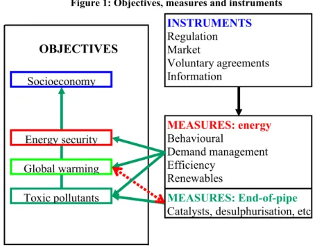
In order to change behaviour, instruments may be deployed. These may be catego-rised as regulation (e.g. emission standards), market (e.g. emission taxes), volun-tary agreements (e.g. CO2 emissions of vehicles, and information (e.g. appliance efficiency labelling). There is no discussion in this report of the instruments that might be deployed to implement the physical measures. The next Figure illustrates how instruments effect measures in order to meet policy objectives.

(14)

Figure 1: Objectives, measures and instruments OBJECTIVES Energy security Socioeconomy Global warming Toxic pollutants MEASURES: energy Behavioural Demand management Efficiency Renewables INSTRUMENTS Regulation Market Voluntary agreements Information MEASURES: End-of-pipe

Catalysts, desulphurisation, etc

Important to an integrated policy are options such as more demand management, energy efficiency and use of low impact fuels as compared to the 'official' scenar-ios. Historically, the emphasis has been on EOP options for the control of non-GHGs. This is partly because large reductions in some pollutants, such as SO2, could be achieved at low cost with EOP technologies implemented through regula-tion such as the Large Combusregula-tion Plant Directive, without requiring large changes to the energy economy; and because, in general, global warming and greenhouse gases have not been regulated by EU legislation historically. However, as tighter limits have pushed up the costs of EOP options, and concern about global warming has increased, and some political commitment to controlling it has followed within individual Member States and the EU as a whole, there has been a greater emphasis on developing integrated policies that address the multiple environment problems of global warming and air pollution. This is particularly because measures to con-trol greenhouse gases generally also reduce air pollutants, and thereby stringent targets for both can be achieved at a lower total cost than addressing each sepa-rately.

'End-of-pipe' abatement technologies generally decrease energy efficiency and some produce wastes, and decreasing energy efficiency usually increases carbon dioxide emissions. For example: flue gas desulphurisation may decrease the effi-ciency of electricity generation by 5% and require limestone inputs and produce waste gypsum; carbon sequestration by pumping CO2 into depleted reservoirs can decrease energy efficiency by 10-35% and hence increase primary CO2 production. Furthermore, in addition to abating greenhouse gas emissions, NEOP options gen-erally decrease the emissions of air pollutants such as SO2 and NOx because fossil fuel combustion is reduced. NEOP options facilitate greater emission abatement

(15)

than is possible with EOP measures alone, and the total combined cost of meeting greenhouse gases and air pollutant targets is generally less than in scenarios which do not include the extensive use of NEOP.

NEOP solutions, with the exception of switching between fossil fuels, also reduce dependence on fossil fuels and improve security of supply. Natural gas and oil are especial cause for concern because the remaining world reserve lives are measured in decades. The use of gas, particularly for electricity generation, has been an im-portant option for reducing both acid and CO2 emissions. Now, the depletion of European gas and oil fields gives concern about energy supply security because of the need to import, and causes pressure to increase the use of indigenous fuels with environmental disadvantages, such as coal.

1.1. This study

The basic remit of this study is to produce energy scenarios for the twenty-five European Union countries such that the total carbon dioxide emissions from fossil fuel combustion are reduced by 30% or more by 2020 as compared to 1990. These scenarios assume extra CO2 abatement measures being introduced in 2008, and would therefore have ten years at most to take effect to achieve a reduction in 2020. Judgements as to which measures to introduce have been based on technical feasibility, cost effectiveness and speed of introduction.

One specific aim here is to develop energy scenarios with the SEEScen (Society Energy and Environment Scenario) model that has a detailed implementation of NEOP measures such as insulation in buildings or the selection of cars with lower power. The scenarios are input to the GAINS model and the air pollution emissions and EOP costs assessed; this analysis is in chapter 7. Apart from the defined envi-ronmental objectives pursued in the scenarios, there are other objectives such as energy security which are important, but these are not generally addressed explic-itly or in detail.

The energy flows in these scenarios are put into the same categories as in IIASA’s GAINS model which may then be used to generate EOP costs. The GAINS model may then be used to find optimal allocation of EOP measures to achieve given reduced levels of acid deposition and ground-level ozone, but this is not part of the work in this report.

The work is in two basic parts: first, develop one energy scenario for each EU25 country in which CO emissions are significantly controlled for the period 2005 to

(16)

I. Update databases.

II. Set targets for CO2 in 2020.

III. Set constraints on NEOP measures. Particularly important are as-sumptions about nuclear power.

IV. Construct scenarios so as to meet energy goals such as minimising net energy trade into the EU, so as not to effectively ’export’ energy and environment problems, and to improve energy security. The scenarios utilise a mix of NEOP measures such that goals are met for each EU25 country. A model called SEEScen (Society, Energy and Envi-ronment Scenario) will be used. The scenarios assume that extra CO2 abatement measures were introduced in 2008, and it is from this date that the scenarios would diverge.

V. Output the scenario energy flows and costs for each country, and for the EU25 as a whole.

VI. Transfer energy data into a form suitable for IIASA's GAINS model, and run the GAINS model.

The scenarios cover the EU25. Countries and international standard 2 and 3 letter codes are given in the next Table.

Table 2 EU25 country codes

Entity ISO 2 ISO 3 Entity ISO 2 ISO 3

Austria AT AUT Latvia LV LVA

Belgium BE BEL Lithuania LT LTU

Cyprus CY CYP Luxembourg LU LUX

Czech Republic CZ CZE Malta MT MLT

Denmark DK DNK Netherlands NL NLD

Estonia EE EST Poland PL POL

Finland FI FIN Portugal PT PRT

France FR FRA Slovakia SK SVK

Germany DE DEU Slovenia SI SVN

Greece GR GRC Spain ES ESP

Hungary HU HUN Sweden SE SWE

Ireland IE IRL United Kingdom GB GBR

Italy IT ITA

1.2. Scope of emissions

The energy model SEEScen projects the demands and energy consumption for all activities in society, including international aviation and shipping. Currently the energy use and emissions from international aviation and shipping — so called bunker fuels — are excluded from the Kyoto Protocol.

“In accordance with the IPCC [Intergovernmental Panel on Climatic Change] Guidelines for the preparation of greenhouse gas (GHG) inventories and the UNFCCC [United Nations Framework Convention on Climate Change] reporting

(17)

guidelines on annual inventories, emissions from international aviation and mari-time transport (also known as international bunker fuel emissions) should be cal-culated as part of the national GHG inventories of Parties, but should be excluded from national totals and reported separately. These emissions are not subject to the limitation and reduction commitments of Annex I Parties under the Convention and the Kyoto Protocol.”

http://unfccc.int/methods_and_science/emissions_from_intl_transport/items/1057.p hp

1.3. EU carbon dioxide emission targets

This section summarises EU25 CO2 emissions and the setting of emission targets for 2010 and beyond. Fossil fuel CO2 emissions data are taken from the Carbon Dioxide Information Analysis Centre (CDIAC) for data published in 2005 (CDIAC, 2005).

The Figure below shows the distribution of fossil fuel CO2 emissions in 2000 across the EU25. The 'Big Six’ (Germany, UK, Italy, France, Poland and Spain) accounted for about 75% of EU25 emissions, with Germany and the UK account-ing for about 40% of emissions.

Figure 2 EU25 Fossil fuel CO2 emissions in 2000

AUT BEL DNK FIN FRA DEU GRE IRE ITA LUX NLD PRT ESP SWE GBR HUN CZR EST LTU LVA POL SLV MLT SLK CYP

(18)

Under the Protocol, the EU15 (the 15 countries that were Members of the EU at the time of ratification of the Protocol) is committed to reducing its greenhouse gases emissions by 8% below 1990 levels during the first commitment period from 2008 to 2012. This target is shared between the 15 Member States under a legally binding burden-sharing agreement, which sets an individual emissions target for each Member State. Of the ten Member States that acceded on 1 May 2004, eight have individual reduction targets of 6% or 8% under the Kyoto Protocol. Only Cyprus and Malta do not have Kyoto targets.

The next Table summarises the commitments. Table 3 EU greenhouse gas emission burden sharing

Region Target Emissions in 2003

2008-2012 with existing policies & measures (PAMs)

2008-2012 with addi-tional PAMs and/or Kyoto mechanisms EU15 8.00% -1.70% -1.60% -9.30% EU25 - -8.00% -5.00% -11.30% Austria 13.0% 16.6% 8.7% -18.1% Belgium -7.5% 0.6% 3.1% -7.9% Denmark 21.0% 6.3% 4.2% na Finland 0.0% 21.5% 13.2% 0.0% France 0.0% -1.9% 9.0% -1.7% Germany 21.0% -18.5% -19.8% -21.0% Greece 25.0% 23.2% 34.7% 24.9% Ireland 13.0% 25.2% 33.4% na Italy -6.5% 11.6% 13.9% -3.7% Luxembourg 28.0% -11.5% -22.4% na Netherlands -6.0% 0.8% 3.5% -8.5% Portugal 27.0% 36.7% 52.1% 42.2% Spain 15.0% 40.6% 48.3% 21.0% Sweden 4.0% -2.4% -1.0% - United Kingdom 12.5% -13.3% -20.3% - Czech Republic -8.0% -24.3% -25.3% -26.5% Estonia -8.0% -50.8% -56.6% -60.0% Hungary -6.0% -31.9% -6.0% - Latvia -8.0% -58.5% -46.1% -48.6% Lithuania -8.0% -66.2% -50.6% - Poland -6.0% -32.1% -12.1% - Slovakia -8.0% -28.2% -19.7% -21.3% Slovenia -8.0% -1.9% 4.9% 0.3% Cyprus Malta Source: Europa, 2006

(19)

The indications are that the EU25, in aggregate, will meet its 2010 Kyoto commit-ment, but only with additional measures and Kyoto mechanisms.

In 2003, the most recent year for which data is available, the EU15 had re-duced its emissions by 1.7%. EU-wide emissions were down by 8%. Projections show that additional policies and measures planned by the Member States but not yet implemented and use of the Kyoto flexible mechanisms will take EU15 emis-sions to 9.3% below 1990 levels by 2010 - more than enough to meet the 8% reduc-tion target - while EU25 reducreduc-tions will reach 11.3%. Only six Member States were not on track to meet their targets: Denmark, Ireland, Italy, Portugal, Slovenia and Spain (see annex for details).

1.3.1. Post 2010 targets

This study is investigating emission control for years later than 2010, with a par-ticular focus on 2020. The question then is what the overall EU25 targets for GHG should be, and how these are allocated to individual countries.

First, we define the scope of GHG covered in terms of gases and sectors, and the geographical inclusion.

x GHG included. Only CO2 from fossil fuel burning is included in the tar-gets, and it is assumed that this CO2 emission has to meet the same per-centage targets as the basket of GHGs. CO2 arising from other combus-tion (e.g. forestry), or processes (e.g. cement manufacture), and other gases such as methane, are not included in the targets developed below. x Measures in non-EU countries. In this study, it is assumed that targets are

met using emission control with measures within EU25 countries only; GHG control achieved by measures outside the EU25, through mecha-nisms such as FlexMex or CDM is not included.

Then we need to make assumptions about targets beyond Kyoto, for 2020 in par-ticular. The Presidency Conclusions of the Council of The European Union (CEU, 2005) stated:

The European Council emphasises the EU's determination to reinvigorate the in-ternational negotiations by:

– exploring options for a post-2012 arrangement in the context of the UN climate change process, ensuring the widest possible cooperation by all countries and their participation in an effective and appropriate international response;

- developing a medium and long-term EU strategy to combat climate change, con-sistent with meeting the 2ºC objective. In view of the global emission reductions

(20)

lieves that, in this context, reduction pathways for the group of developed countries in the order of 15-30% by 2020, compared to the baseline envisaged in the Kyoto Protocol, and beyond, in the spirit of the conclusions of the Environment Council, should be considered. These reduction ranges will have to be viewed in the light of future work on how the objective can be achieved, including the cost-benefit as-pect. Consideration should also be given to ways of effectively involving major energy-consuming countries, including those among the emerging and developing countries;

– promoting cost-efficient measures to cut emissions.

Targets for reduction in total EU25 1990 fossil CO2 by the year 2020 are set. The question then is how the required reductions for the whole EU25 might be allo-cated to individual Member States.

It was originally intended to develop scenarios such that EU25 and individual country targets were met, with burden sharing through country targets devised with principles of equity. However, the differing demands and energy resources of countries, and the time required to detail policies country by country, has meant this has not been possible in this work to propose burden sharing of either the CO2 or renewable energy supply targets.

It is anticipated that quantifying burden sharing will require lengthy and complex analysis and negotiation. Therefore, the CO2 reductions and renewable energy component of each country has been set in the scenarios by judgements about the further economic potential of energy efficiency and energy sources based on data available to the study.

Elements of the intended approach to burden sharing are set out in Appendix 1.

1.3.2. Energy trade and carbon emission

The aim is to achieve environmental and other objectives at least cost. Ideally, this would mean optimising energy strategy across all demand and supply options and all countries of the world. It makes economic sense to import renewable energy resources into a country if they can be obtained at lower cost and so, in a globally optimised strategy, trade in energy would occur. The economic advantage of trade is tempered by considerations of energy security.

The existing databases and models are not adequate for a global optimisation of both demand and supply, particularly when there is a large renewable component of supply. SEEScen works country by country and does not endogenously account for trade between countries. However, the net trade for each country is calculated and this may be summed across the EU to find trade for the whole region, although this give no indication of trade between pairs of EU countries. Trade and energy security is discussed in section 6.3.1.

(21)

Furthermore, in the particular scenarios explored here, exogenous assumptions concerning nuclear generation are made, some following those in the PRIMES scenarios. The assumptions about nuclear generation are often partially based on current political intents in each country, rather than on technology appraisal. The assumed nuclear generation represents a significant fraction of the EU25 renewable electricity generation potential. Countries with assumed new nuclear generation and significant renewable electricity sources become exporters of electricity in the SEEScen scenarios.

How is traded energy accounted for in carbon? For the fossil fuels, the carbon emissions of fossil fuels consumed within that country (apart from international transport fuels) are calculated simply and accurately using coefficients of carbon per GJ/tonne/therm. Fossil fuel exports do not appear in the carbon balance of the exporting country because carbon emissions from these appear in the importing, consuming countries.

The carbon content of generating electricity depends on how the electricity is gen-erated and this often varies from hour to hour. Emissions from generation within a country appear in the national carbon balance. Unlike fossil fuels, the carbon con-tent of electricity at the point of consumption is zero. The question is how to ac-count for electricity trade and emissions. The simplest option is to assign zero car-bon to traded electricity because the exporting country will be benefiting economi-cally, earning money from those exports, and the importing country will be dis-benefitted in trade balance, though benefiting overall by purchasing energy more cheaply than it can generate it. However, this approach has limitations when con-sidering the net carbon emissions of a region and emission targets.

This issue is unresolved in this report, but is discussed in section 6.3.1 with refer-ence to particular scenarios; in the base scenario studied here, the EU25 has net exports of electricity and net imports of fossil gas and oil.

1.4. The scenarios

Six scenarios were modelled: a central scenario with a 30% reduction in EU25 CO2 emission by 2030, and five variant scenarios with various combinations of NEOP measures and different assumptions about nuclear power. The scenarios are gener-ally labelled Region: Percentage reduction fossil CO2 from 1990: reduction date: Nuclear (new nuclear as in PRIMES)/ No Nuclear (no new nuclear). The scenario of central focus is labelled EU30pc20N, meaning Europe Union: 30% reduction from 1990 by 2020; nuclear generation as assumed in PRIMES.

(22)

Table 4 Scenarios Label Target: % CO2 reduction from 1990 Target: Reduction date Nuclear energy NEOPs

EU30pc20N 30 2020 New Mix

EU40pc20N 40 2020 New Mix

EU30pc20NN 30 2020 No new Mix

TecNN No new Maximum technology

BehNN No new Maximum behavioural

TecBehNN No new Maximum technology and

behaviour

A number of points should be emphasised :

x The starting point of a scenario is the last year of historical data which usually take 2 or more years to verify and make available; for example, the International Energy Agency (IEA) energy data for 2004 were avail-able in the summer of 2006. Thus scenarios do not start from the present and when analysing near term targets for 2010 or 2020 the error can be large. New historical data arrive each year, and so the starting point of the scenarios developed here is different from other scenarios more than a year old.

x All historical databases almost certainly contain numerical and categori-cal errors.

x There are no fixed rates of change for measures. Coal fired power sta-tions might be decommissioned after 40 years, or after 20.

x There are large uncertainties in all predictions of economic and social development, and technological innovation.

For these reasons, the scenarios will not be accurate in absolute terms. What is important, therefore, are the measures that the scenarios indicate that might be beneficent in environmental, economic and other terms.

(23)

2. Modelling the Scenarios

2.1. SEEScen model

The scenario model is called SEEScen (Society Energy and Environment Sce-nario). It is designed to produce energy scenarios which may be used in the analy-sis of environmental impacts. It is a simulation model: assumptions about policy options are input the model and it calculates the outcomes in terms of energy, costs and emissions. It does have a single year optimisation mode, but that is not used here, partly because of the conceptual problem of assigning costs to behavioural change.

The structure of the model is shown schematically in the next Figure. Figure 3 SEEScen model overview

HISTORY FUTURE COSTS INPUTS / ASSUMPTIONS IMPACTS ENERGY IEA data Energy Population, GDP Other data Climate, insulation... Delivered fuel

End use fuel mix End use efficiency

Delivered fuel by end use Useful energy Socioeconomic Useful energy Delivered energy Lifestyle change Demand management

End use fuel mix End use efficiency

Conversion

Primary energy Supply efficiency

Emissions Capital

Runnin Distribution losses

Supply mix

(24)

The IEA has assembled a database of the energy statistics for most countries of the world (IEA, 2006), the most recent data year available for this study being 2004. These data have been compiled into country energy balances. These balances in-clude sectoral data for the consumption and production of fossil fuels, hydro, nu-clear, geothermal and other renewables, electricity and heat. This database also includes GDP and population.

The consumptions of delivered fuel in 2004 are allocated to eleven end uses as shown in the next Table– they are ordered by temperature. Some of these end uses are generally regarded as electricity specific; others can utilise heat from cogenera-tion or other sources such as solar energy (as opposed to fossil fuels or electricity). These features are also shown in the Table uses marked ‘e’ can practically only use electricity.

Table 5 End uses and supply restriction

End use Electricity specific

Motive power e Electrical equipment e Process work Lighting e Process heat (>120C) Process heat (<120 C) Cooking Water heating Space heating Space cooling e Refrigeration e

Delivered fuels by end use are multiplied by a set of efficiencies to produce useful energy consumed for the eleven end uses such that the delivered fuels calculated match historically recorded. This establishes useful energy consumption for the last year for which there are IEA data (2004).

These useful energy data are then projected into the future using ‘energy activity functions’ based on estimates of future population, households and GDP data from other sources. These estimates may be endogenous, or as in this case, exogenous, taken from the PRIMES scenarios. Every scenario for a particular country assumes the same demographic and economic changes - i.e. these are invariant. In these scenarios, further exogenous data are used for transport demand and nuclear gen-eration.

The basic projection of useful energy is then modified according to control meas-ures changes in behaviour (Be) such as car downsizing, and demand management (DM) such as insulation.

(25)

Useful energy demands are allocated to an end use supply mix. For example; water heating might be allocated to a mix of energy converters including solar heating, electric heat pumps and CHP district heating.

Energy deliveries to the end user are calculated by dividing the useful energy by the appropriate projected efficiencies of end use converters.

After adding on distribution losses, and allowing for imports and exports the re-quirements for domestic inland energy supply may be found.

Supply side efficiency improvements and fuel switching are then applied so that the fuel used in energy supply industries may be calculated.

If the potential electricity production from non fossil sources is greater than domes-tic demand, the surplus is exported. This electricity could be used to replace carbon based generation in another country. SEEScen accounts for exports.

Emissions and costs are calculated for each component of the energy system.

2.2. Comments on the SEEScen model

The SEEScen modelling system has been developed for specific purposes. Like all models it has strengths and weaknesses.

Strengths include:

x It is a ‘bottom’ up model with physical descriptions of demand, demand management and technologies.

x It can be used to rapidly identify the technical potential of different pol-icy options.

x It can be used to generate scenarios for any country for which there are IEA data, which is all major countries of the world. Since the IEA data are published annually, the model always has a recent fuel use database to base projections on. Furthermore, the IEA collate a number of other statistical series which are useful inputs to the modelling process. x The model can be used to rapidly explore the effects of different

pro-grammes in energy strategies for many countries in any geographical or political grouping. The profile of programmes, in terms of change in fuel use and the time and rates of change can be easily altered. The pro-grammes can be applied in any combination and thus the effect of each can be isolated and analysed separately.

(26)

x It does not incorporate the responses of economic agents to costs and prices with elasticities.

x It does not include consideration of how technical changes to the energy system might be brought about by instruments such as taxation or regula-tion.

SEEScen does calculate the emissions of air pollutants, though the emission factors require development. The model can be used to arrive at the total additional cost of reaching a set of environmental objectives encompassing targets for the emissions of energy related greenhouse gas and air pollutant emission.

(27)

3. Exogenous Assumptions Used

in the Scenarios

3.1. Background

The system of people, ecosystems, energy and the environment is one global inter-connected system, but it is not presently possible to model it all in any useful de-tail. Accordingly, in all modelling exercises, there are data input to the model – exogenous data or assumption – and data calculated endogenously through the relationships between variables in the model. The starting point for these energy scenarios is to compile assumptions about the basic drivers of energy consumption – population, households, GDP, and sectoral economic activity. Other exogenous assumptions include international energy prices and particular policies affecting sectors such as buildings, transport and electricity generation, but these are not explicitly included here.

Such assumptions are exogenous to many energy models. In reality, energy and environment scenario outcomes will affect some or all of these exogenous assump-tions: for example, lower CO2 emission generally results from lower fossil fuel consumption which causes fossil fuel prices to be lower than in a higher consump-tion scenario; and energy prices affect activities, GDP and household formaconsump-tion, if only marginally.

Some exogenous inputs, such as transport demand are dependent on a range of policies. For example, the distance travelled by people each year depends on a complex of factors such as land use patterns, road provision, city traffic cordons, and transport pricing. The distance travelled may be influenced by policies in order to meet aims such as reduced congestion, economic savings, and a safer, less pol-luted local environment; as well as less CO2 emission. (For example: the London congestion charge does all these things.) In other words, these measures may be called NEOP measures for the control of distance travelled and thereby CO2 emis-sion.

The aim here is to use certain assumptions about drivers and other key measures made in the PRIMES scenarios, but make different assumptions about NEOP measures so as to reduce CO2 emission to lower levels than in the PRIMES scenar-ios. There is a difficulty here in that some measures are explicitly included in SEEScen, but are not, as far as is known, in PRIMES; for example, SEEScen has a explicit data concerning the size and insulation levels for dwellings, and a model of

(28)

The basic future socioeconomic context and energy scenarios for Europe are de-scribed in several documents, with these being useful general descriptions. These were chosen from those publicly available and documented in mid 2006 (other scenarios have been produced since then); they are as follows:

x European Commission Directorate-General for Energy and Transport, September 2004, European Energy and Transport Scenarios on Key Drivers. (DGTren, 2004)

http://europa.eu.int/comm/dgs/energy_transport/figures/scenarios/doc/su mmary.pdf

x DGTren (European Commission Directorate-General for Energy and Transport), January 2003, European Energy and Transport Trends to 2030. (DGTren, 2003)

http://www.eu.int/comm/dgs/energy_transport/figures/trends_2030/1_pre f_en.pdf

x Using these scenarios as background, the PRIMES model was used to develop detailed scenarios, as described in Long-Term Scenarios For Strategic Energy Policy of the EU (NTUA, 2005). This may be downloaded from:

http://ec.europa.eu/environment/air/cafe/general/keydocs.htm x For this work, two PRIMES scenarios are used: No Climate Policies

(NCLP); and With Climate Policies (WCLP). For each EU25 country, data for two scenarios are given and may be downloaded from this web site:

www.europa.eu.int/comm/dgs/energy_transport/figures/trends_2030/inde x_en.htm

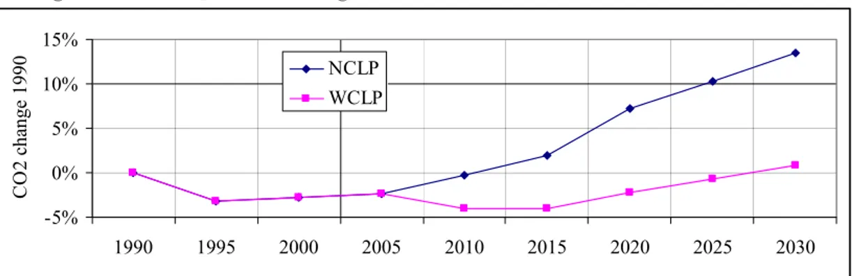
PRIMES calculates CO2 emission from fossil fuel use. The next Figure shows the index of total CO2 emission in two scenarios. It is to be noted that neither scenario meets the EU25 target for 2010 (excluding FlexMex) and that both show increasing emission after 2015. It may be that the inclusion of non-CO2 gases, the 2010 targets are met.

Figure 4 EU25 CO2 emission change in the NCLP/WCLP PRIMES scenarios

-5% 0% 5% 10% 15% 1990 1995 2000 2005 2010 2015 2020 2025 2030 C O 2 c h ange 199 0 _NCLP WCLP

(29)

It is to be noted that if the total fossil fuel energy is higher than required by GHG targets, the cost of reducing NEC emissions to a certain level will probably be higher; moreover, the possibilities of reduction will probably be less, thus lowering economically achievable emission targets.

These PRIMES scenarios extend out to 2030. Any data presented here for years after that date are simple extrapolations. In general, key exogenous assumptions input to the NCLP and WCLP scenarios are identical, or have small differences as summarised in the next Table.

Table 6 Exogenous assumptions — variation by scenario

Item NCLP/WCLP variation

Socioeconomic Population None

Households None

GDP None

Transport Passenger Slight

Freight Slight

Fuel prices Oil, coal, gas None

Nuclear generation Small

3.2. Energy and climate policy dependent

as-sumptions

The following sections briefly describe the assumptions which are adopted from the PRIMES scenarios.

3.3. Demography

The EU25 population is forecast to grow slowly to a peak in 2015, after which it gradually declines.

(30)

Figure 5 Population in millions (M) 0 50 100 150 200 250 300 350 400 450 500 1995 2000 2005 2010 2015 2020 2025 2030 SWE SLV SLK PRT POL NLD MLT LVA LUX LTU ITA IRE HUN GRE GBR FRA FIN EST ESP DNK DEU CZR CYP BEL AUT M

Source: PRIMES NCLP scenario

Increasing wealth and other social changes result in smaller households.

Figure 6 People per household

0 0.5 1 1.5 2 2.5 3 3.5 4 4.5 5 1995 2000 2005 2010 2015 2020 2025 2030 AUT BEL CYP CZR DEU DNK ESP EST FIN FRA GBR GRE HUN IRE ITA LTU LUX LVA MLT NLD POL PRT SLK SLV SWE people/HH

Due mainly to the decline in household size, there is an increase in the number of households. The number of households is an important determinant of energy con-sumption because energy use per person generally increases with decreasing household size: this is because building floor and envelop area per person

(31)

increases, and the ownership and use of many energy using technologies (e.g. cars, refrigerators) is strongly related to the number of households as well as the number of people. Figure 7 Households 0 50 100 150 200 250 1995 2000 2005 2010 2015 2020 2025 2030 SWE SLV SLK PRT POL NLD MLT LVA LUX LTU ITA IRE HUN GRE GBR FRA FIN EST ESP DNK DEU CZR CYP BEL AUT M

3.4. Economy

Wealth is an important driver of energy consumption. Once levels of wealth are sufficient that basic needs such as adequate thermal comfort are met, wealth may be spent on inessential or leisure needs some of which, such as air travel, more powerful cars, or larger houses, increase energy consumption and associated emis-sions. Conversely, there can be decoupling of wealth and energy and emissions for some commodities and services because of saturation. For example; once living temperatures rise to a comfortable maximum, increasing wealth will not result in higher temperatures and associated energy and emissions. The surplus wealth ‘saved’ by this saturation might be spent on something with a lower emission per Euro, such as jewellery, or something with a higher emission, such as air travel. A steady growth in GDP is forecast in the PRIMES scenario. GDP growth is higher in the services sector than the industrial sector. The next Figure shows GDP in billion of Euros (2004).

(32)

Figure 8 GDP 0 5000 10000 15000 20000 25000 30000 19 90 19 95 20 00 20 05 20 10 20 15 20 20 20 25 20 30 20 35 20 40 20 45 20 50 G E u ro2 00 4 SWE SVN SVK PRT POL NLD MLT LVA LUX LTU ITA IRL HUN GRC GBR FRA FIN EST ESP DNK DEU CZE CYP BEL AUT Source: PRIMES NCLP scenario

3.5. Demand

Of fundamental importance to energy scenarios are the demands for energy. These arise in two ways: first, from direct consumer demand for energy-based services, such as space heating or transport; and second, through the energy required by industry and services sectors to provide these services and commodities.

3.5.1. Transport

The PRIMES NCLP scenario assumes a steady increase in distance travelled per person and thence an increase in total distance for the population of about 44% over the period 2005 to 2030.

(33)

Figure 9 Passenger transport per capita 0 5000 10000 15000 20000 25000 1995 2000 2005 2010 2015 2020 2025 2030 AUT BEL CYP CZR DEU DNK ESP EST FIN FRA GBR GRE HUN IRE ITA LTU LUX LVA MLT NLD POL PRT SLK SLV SWE km

Figure 10 Passenger transport (billion p.km)

0 1000 2000 3000 4000 5000 6000 7000 8000 9000 1995 2000 2005 2010 2015 2020 2025 2030 SWE SLV SLK PRT POL NLD MLT LVA LUX LTU ITA IRE HUN GRE GBR FRA FIN EST ESP DNK DEU CZR CYP BEL AUT Gpkm

(34)

Figure 11 Passenger transport by car in billion passenger km (Gpkm) 0 1000 2000 3000 4000 5000 6000 7000 8000 9000 1995 2000 2005 2010 2015 2020 2025 2030 SWE SLV SLK PRT POL NLD MLT LVA LUX LTU ITA IRE HUN GRE GBR FRA FIN EST ESP DNK DEU CZR CYP BEL AUT Gpkm

Freight transport grows faster than passenger transport, increasing by 68% over the period 2005 to 2030.

Figure 12 Freight transport in billion tonne km (Gtkm)

0 500 1000 1500 2000 2500 3000 3500 4000 4500 1995 2000 2005 2010 2015 2020 2025 2030 SWE SLV SLK PRT POL NLD MLT LVA LUX LTU ITA IRE HUN GRE GBR FRA FIN EST ESP DNK DEU CZR CYP BEL AUT Gtkm

These exogenous assumptions about transport growth are critical to the prospects for CO2 emission and for the consumption of fossil liquid fuels for transport, which are the most difficult to replace. The transport demand forecasts used by PRIMES

(35)

are made using functions of income, consumer preference and relative prices. These may not fully account for other factors, including saturation effects. For example, in the UK, travel distance per person per year (excluding interna-tional travel) has not changed significantly for the past ten years. It is notable that the average speed of travel and time taken have shown signs of levelling off as is shown in the next Figure. One probable reason for this is greater congestion on the road network. In addition, changes in fundamental drivers such as land use patterns and distance between home and work place. Such effects mean that the functions fitted to past consumption will not necessarily produce accurate forecasts. The UK data suggest that if saturation effects are not accounted for, that the exogenous demand projections used may be too high.

Figure 13 UK passenger travel trends

15 17 19 21 23 25 27 29 31 33 35 1970 1980 1990 2000 2010 kph/ km pe r da y -0.6 0.7 0.8 0.9 1.0 1.1 h r s/d a y Speed km/day Hrs/day

Source: National Travel Survey (DfT, 2006)

Furthermore, changes to transport demand and its allocation to different modes may be called measures, and can be influenced with instruments such as car restric-tion, congestion charging, teleworking, etc. For these reasons, to take the PRIMES transport scenarios as exogenous fixed projections means that the full range of measures is not available. Therefore the base demand for transport (passenger kilometres and freight tonne kilometres) is taken from PRIMES, but this may be modified in the scenarios by demand management and modal change.

(36)

on Government policies, which have been in flux in most EU25 States for some years.

The next Figure shows the historic profile of commissioning in the EU25 countries with a peak rate of commission in the mid 1980s leading to a peak installed capac-ity around 2000. The operational capaccapac-ity of existing plant in the future depends on operating lives; and the Figure shows the profile of operating capacity assuming a lifetime of 35 years.

Figure 14 Historical and projected existing nuclear capacity

0 20000 40000 60000 80000 100000 120000 140000 1 955 ₁960 ₁965 ₁970 ₁975 ₁980 ₁985 ₁990 ₁995 ₂000 ₂005 ₂010 ₂015 ₂020 ₂025 ₂030 ₂035 ₂040 ₂045 ₂050 M W SVN SVK LTU HUN CZE SWE NLD ITA GBR FRA FIN ESP DEU BEL

Source: Platts power plant database, 2007.

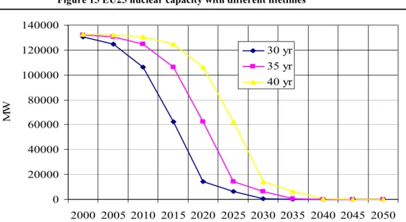
Given that planning and constructing a nuclear power station takes 5-10 years and that it would take a considerable time to ramp up to a programme of parallel station construction, few new stations will be operating by 2020 whatever the assumed government policies. Therefore, for 2020, the most significant parameter is the assumed lifetimes for existing plants. The next Figure depicts the EU25 operational nuclear capacity of existing plants assuming 30, 35 and 40 year lifetimes; the ca-pacity operating in 2020 is 14 GW, 62 GW and 106 GW respectively for these lifetimes.

(37)

Figure 15 EU25 nuclear capacity with different lifetimes 0 20000 40000 60000 80000 100000 120000 140000 2000 2005 2010 2015 2020 2025 2030 2035 2040 2045 2050 M W 30 yr 35 yr 40 yr

Assuming different lifetimes, the next Figure gives the approximate fractions of EU25 total CO2 emission avoided using nuclear power, assuming it generates at a 75% annual capacity factor and displaces fossil generation at 0.43 kg CO2/kWh. This is representative of gas combined cycle gas turbine (CCGT); if it were coal, the emission avoided would be approximately doubled. The fraction ranges from about 0.5% to 5.5% in 2020, so lifetimes and the corresponding generation from existing nuclear power stations are critical for meeting targets in 2020. This sug-gests there will be a significant effort to extend nuclear station lifetimes.

Figure 16 Avoided CO2 emission because of nuclear power

1% 2% 3% 4% 5% 6% 7% 8% % EU 25 C O 2 ( 1990 ) 30 yr 35 yr 40 yr

(38)

Figure 17 Nuclear capacity projection 0 20000 40000 60000 80000 100000 120000 140000 160000 1995 2000 2005 2010 2015 2020 2025 2030 SWE SLV SLK PRT POL NLD MLT LVA LUX LTU ITA IRE HUN GRE GBR FRA FIN EST ESP DNK DEU CZR CYP BEL AUT MW

There is slightly more nuclear capacity and generation In the WCLP scenario than in the NCLP scenario. Plainly, the assumptions about nuclear power are critically affect atmospheric emissions.

Figure 18 Nuclear capacity projections

0 20000 40000 60000 80000 100000 120000 140000 160000 1995 2000 2005 2010 2015 2020 2025 2030 MW NCLP WCLP

Source: PRIMES NCLP / WCLP scenarios

3.7. International fossil fuel prices

International fuel prices are the same in the NCLP and WCLP scenarios. In reality, the price of a fuel will be higher in a scenario in which more of that fuel is con-sumed. Accordingly, prices should generally be higher in the NCLP scenario than

(39)

the WCLP scenario. SEEScen uses fuel prices to calculate the total costs of energy scenarios, but it does not model the effect of fuel prices on outcomes such as trans-port demand or mode, or generation mix — these are exogenously specified.

Figure 19 International fossil fuel price projections

0 50 100 150 200 250 1990 1995 2000 2005 2010 2015 2020 2025 2030 E u r o '0 0 0 /t o e oil gas coal

(40)

4. Emission Control Measures

The general categories of NEOP and EOP emission control measures were set out in Table 1. These are briefly described below and expanded in Table 7.

Behaviour

Behavioural changes relate to demand, and the choice and use of technologies. Travelling less or heating a house to a lower temperature reduces energy consump-tion and emissions. Choosing the most fuel efficient car currently marketed, will reduce energy use and CO2 emissions by over 50% as is shown below. Driving vehicles more slowly on motorways could reduce emissions on those roads by 10-20%. In Energy, Carbon Dioxide and Consumer Choice (1992), Barrett gives an overview of some of the behavioural options deployed in the SEEScen model.

Demand management

Demand management is defined as energy savings achieved through measures such as insulation, ventilation control, heat recovery, improved energy system controls, low mass vehicles, and low flow showers. Demand management is applied in the sectors of end use or final consumption, and can apply to new or existing technolo-gies (e.g. an existing building.).

Efficiency of energy conversion

The efficiency of energy conversion is defined as the ratio of useful energy output from a technology to the fuel energy input - it thus refers mainly to energy tech-nologies such as boilers and power stations. Efficiencies can be improved in end use sectors (boilers, cookers, lights etc.) and in energy supply (power stations, refineries etc.). The potential efficiency gains of technologies in general vary ac-cording to the fuel used. For example, the potential improvement in efficiency for electric water heating is assumed to be 15%, less than the 30-50% which might be expected for water heating with oil.

Fuel switching

Changing the mix of fuels supplied directly to consumers and to the producers of secondary fuels such as electricity and heat can reduce carbon emissions. This may be done in two ways:

x Switching to inherently lower carbon fuels: the order of carbon emission per energy content is renewable and nuclear (zero), and then fossil natu-ral gas, petroleum and coal.

x Switching to delivered fuels which reduce emissions from the energy system as a whole. This includes switching from electricity to gas where marginal electricity supply is from fossil fuelled electricity only (i.e. non cogeneration) stations; switching to heat where heat is supplied by co-generation or efficient heat only plant.

(41)

The amount of switching possible is limited by the technical and economic poten-tial for different energy forms in different countries, and the rate at which energy mixes may be changed.

To implement the policy options to different degrees in the scenarios, decision variables are set and are input to SEEScen. Some decision variables control several measures. For example: the decision variable BePMod in the Table below controls the modal mix of passenger transport, and shifting a fraction of passenger km from car to bus and rail; FMSup controls the change in fuel supply mix covering all fossil and renewable fuels.

Table 7 Emission control measures and decision variables

Class Examples of measures Rate

yrs

Decision variable name

Effective comfort temperature in buildings 10 BeTi

Passenger transport demand management 20 BeTPass

Aviation transport demand management 15 BeAvi

Passenger mode; from car to bus/rail 20 BePMod

Freight mode; from truck to rail 25 BeFMod

Downsizing cars 15 BeCar

Behaviour

Speed reductions on motorways, aircraft 5 BeSpeed

Transport load factor 20 DMTLF

Demand management in transport 30 DMTra

Building insulation and ventilation control 40 DMBui

Demand mana-gement

Demand management in non-residential sectors

30 DMInd Shift to electric vehicles, CHP and renewables

in end use sectors

35 FMDel

Fuel mix

Shift to CHP and renewables in supply sectors 40 FMSup

Efficiency Improved efficiency of boilers, heat pumps, etc 35 EFDel

Pollution Flue gas desulphurisation, catalytic converters 30 PoAll

In these scenarios, non-biological carbon sequestration, such as the storage of car-bon in exhausted oil or gas reservoirs, is excluded as an option. This is because it impairs energy efficiency, increases primary CO2 emission and is costly. There is a potential risk of leakage. These aspects need further research, but the scenarios developed here indicate that sequestration is not required to achieve large CO2 reductions in Europe.

(42)

x •What is required in order to meet EU25 targets. This is the most impor-tant consideration.

x The degree to which the NEOP measures have already been applied x The potential for further application of NEOP measures.

There are two problems applying the carbon emission reduction options in scenar-ios; knowing accurately what the current situation is, and making assumptions about how much these may be applied in the future.

There is no comprehensive database for Europe covering details such as: x The size and heat loss characteristics of domestic and non-domestic

buildings.

x The average operating efficiencies of boilers, lights, electric motors, power stations, etc.

Therefore there is uncertainty in the starting point of the scenarios, and this leads to uncertainty in future possibilities. If, for example, there are already high levels of insulation in buildings, then future savings will not be large.

The best performance of most technologies is similar across all countries. The maximum efficiency of a gas boiler or a light bulb may be assumed to be the same in Sweden as in Spain. The performance of some technologies, such as heat pumps and solar collectors, is affected by the climate in which they operate, and this varies from country to country.

The potential use of renewable energy resources in each country is uncertain be-cause:

x Data are poor for some countries and some resources. x The amount of energy that may be extracted depends on:

- The marginal costs, which increase steeply with amount extracted. For ex-ample; the cost of wind electricity might double going from a high wind speed onshore site to a distant off-shore site.

- The environmental impacts, which vary widely. For example; the use of biomass waste for CHP might have net environment benefits whereas growing energy crops can have impacts such as decreased biodiversity or increased wa-ter use and pollution.

In any case, it should be recognised that the cost effective scope of the measures, and the rate at which they might be introduced are not fixed values – they can vary widely according to the context of the scenarios. For example:

x The scope for gas substitution in one country will depend on the overall balance of supply and demand in the EU (and indeed elsewhere in Europe and Asia).

x The lifetime of a coal power station will depend, inter alia, on any targets for atmospheric emissions – with tight SO2, NOx and CO2 emission lim-its, the life might be 25 rather than 40 years as earlier replacement with alternative generation becomes more cost effective.

(43)

x The cost effectiveness of end use efficiency depends on the costs of sup-ply, which are scenario dependent. The higher the cost of energy supsup-ply, then the greater increase in end use efficiency is economically justifiable. x Further improvements in technologies may be expected, the speed and

extent of which will depend on factors including policy context. For ex-ample, the expansion and development of renewable electricity sources in the UK has been accelerated by the requirement that a certain fraction of electricity should be derived from non fossil fuel sources.

These comments should be borne in mind when considering the assumptions input to the scenarios concerning cost effective potential for energy efficiency and fuel switching, and the rates of turnover and change assumed for the technologies. Information on the technical scope and economic potential of the NEOP measures explored in the scenarios is drawn from a large number of sources. To comprehen-sively update the information on the measures for each of the EU25 countries is a worthwhile endeavour, but it is beyond the scope of this exercise. Therefore the assumptions about the measures are taken as typical for the EU. From the perspec-tive of EU25 carbon emission, it is important these values are reasonable for the ‘Big Six’ countries as they so dominate total emission.

There is general support for the feasibility of the scenarios in other studies done, for example the European Commission published its Action Plan for Energy

Effi-ciency: Realising the Potential (CEC, 2006a) which said:

The 2006 Spring European Council called for the adoption as a matter of urgency of an ambitious and realistic Action Plan for Energy Efficiency, bearing in mind the EU energy saving potential of over 20% by 2020.

4.2. Rate of implementation of measures

A key issue in this exercise is the rate at which the carbon reduction measures can be introduced; there are only 12 years from the earliest possible introduction of extra measures (2008) to the target year (2020). Table 7 summarises the rates of introduction for the options if average ‘natural’ technology lifetimes assumed. These points should be noted:

x Some technologies have technical lifetimes determined by practically ir-reversible breakdown, such as a light bulb. For some the lifetime is de-termined whether it is cheaper to repair or replace.

(44)

re-technology. This is particularly so for buildings, composed of elements with a wide range of lifetimes: walls (100s of years), windows (30 years), heating systems (20 years). In this instance, it is (arbitrarily) assumed in the scenarios that insulation is retrofitted at a turnover rate of 40 years which is faster than programmes in the UK, but slower than that in Ger-many.

The decision variables are increased with logistic curves to their maximum value for any particular scenario at the rates tabulated, as illustrated in the next Figure. The decision variables labels are given in Table 7. The maximum values for the measures generally vary from scenario to scenario.

Figure 20 Measures introduction with decision variables (GBR)

0% 10% 20% 30% 40% 50% 60% 70% 80% 90% 100% 1990 1995 2000 2005 2010 2015 2020 2025 2030 2035 2040 2045 2050 BeTi BeTPass BeAvi BePMod BeFMod BeCar LSSpeed DMTLF DMTra DMBui DMInd FMDel FMSup EFDel PoAll GBR: EU30pc20N: Decision variables

(45)

5. Results

The SEEScen model was run for all 25 EU countries, and for six scenarios for comparison. It is not possible to present detailed results for every sector and coun-try in this report, as there would be some 100 tables and graphs for each EU25 country. Therefore sample material is given for selected sectors and countries. Because European demands are reasonably homogeneous, this selected material will indicate general trends, though the modelled results depend on details of each country’s climate, population, renewable resources, etc.

Note that:

x Only CO2 emissions from fossil fuel use for energy are included. In these graphs, CO2 emissions are normalised to PRIMES data up to 2000. x International transport (bunker fuel) CO2 emissions are excluded from

national results simply because they are currently excluded from the Kyoto protocol. However, bunker fuel use is included in energy flows as they are part of national energy systems. A separate section discusses in-ternational transport issues.

x The historical IEA energy statistics are sometimes difficult to interpret, particularly concerning electricity and heat generation from public and autoproducer electricity only and combined heat and power stations. In places this leads to erratic historical trends.

5.1. European Union results

Figure 21 shows the carbon emission for the EU25 countries in the EU30pc20N scenario. The black squares show the Kyoto target for 2010 (but note that this does not just apply to CO2) and the 30% target for 2020. In the projection, the EU25 fails to meet the Kyoto target in 2010 for CO2, but then emissions fall steeply such that the 30% target in 2020 is met with a margin — the reduction is 36%. One notable feature is that EU25 carbon emissions are still falling steeply after 2020, this is because the measures take time to fully affect the stock of technologies. This means that the scenarios are quite robust. The reader is reminded that these results would be different if other GHG and measures in other countries such as FlexMex were included.

(46)

Figure 21 EU25 countries carbon emission: SEEScen EU30pc20N scenario 0 500 1000 1500 2000 2500 3000 3500 4000 4500 1990 1995 2000 2005 2010 2015 2020 2025 2030 2035 2040 2045 2050 Mt SWE SVN SVK PRT POL NLD MLT LVA LUX LTU ITA IRL HUN GRC GBR FRA FIN EST ESP DNK DEU CZE CYP BEL AUT Targets COUNTRIES: EU30pc20N : Environment: National: (N) Total : CO2

5.2. Country by country CO

2

emission

The following sequence of Figures gives the sectoral carbon emission for each of the EU25 countries for the EU30pc20N scenarios. Note that there are some prob-lems with historical energy data and the allocation of CO2 emissions with the most important being:

x The allocation of energy and emissions for electricity generation and public CHP. Some historical IEA data for certain countries have apparent problems, e.g. for Poland.

x The allocation of diesel fuel to passenger cars, freight trucks and light duty vehicles (LDVs) is estimated and so are emissions. The partitioning varies widely between countries.

The Table below summarises the graph labelling.

Table 8 Country CO2 labelling

Sector Sub-sector Label

Industry Iron and steel Ind:Iro

Chemical Ind:Che Heavy Ind:Hea Light Ind:Lig Agriculture Ind:Agr Other Oth:oth Services Ser:Ser

(47)

Residential Res:Res

Transport (national) Road passenger Tra(nat):Road: P

Road freight Tra(nat):Road: F

Rail Tra(nat):Rail

Air domestic Tra(nat):Air: Do

Inland water Tra(nat):Other i

Heat supply Auto Hea:Aut

Public Hea:Pub

Electricity Transmission Ele:Tra

Pumped storage Ele:Pum

Generation Ele:Gen

Fuel Processing Fue:Pro

Extraction/distribution Fue:Ext

Figure 22 EU25 country by country CO2 emissions: EU30pc20N

0 10 20 30 40 50 60 70 80 1990 1995 2000 2005 2010 2015 2020 2025 2030 2035 2040 2045 2050 Mt Fue:Ext Fue:Pro Ele:Gen Hea:Pub Hea:Aut Tra(nat):Other i Tra(nat):Air: Do Tra(nat):Rail Tra(nat):Road: F Tra(nat):Road: P Res:Res Ser:Ser Oth:oth Ind:Agr Ind:Lig Ind:Hea Ind:Che Ind:Iro AUT: EU30pc20N: Environment: National: (N) : CO2

40 60 80 100 120 Mt Fue:Ext Fue:Pro Ele:Gen Hea:Pub Hea:Aut Tra(nat):Other i Tra(nat):Air: Do Tra(nat):Rail Tra(nat):Road: F Tra(nat):Road: P Res:Res BEL: EU30pc20N: Environment: National: (N) : CO2

(48)

0 1 2 3 4 5 6 7 8 1990 1995 2000 2005 2010 2015 2020 2025 2030 2035 2040 2045 2050 Mt Fue:Ext Fue:Pro Ele:Gen Hea:Pub Hea:Aut Tra(nat):Other i Tra(nat):Air: Do Tra(nat):Rail Tra(nat):Road: F Tra(nat):Road: P Res:Res Ser:Ser Oth:oth Ind:Agr Ind:Lig Ind:Hea Ind:Che Ind:Iro CYP: EU30pc20N: Environment: National: (N) : CO2

0 20 40 60 80 100 120 140 160 1990 1995 2000 2005 2010 2015 2020 2025 2030 2035 2040 2045 2050 Mt Fue:Ext Fue:Pro Ele:Gen Hea:Pub Hea:Aut Tra(nat):Other i Tra(nat):Air: Do Tra(nat):Rail Tra(nat):Road: F Tra(nat):Road: P Res:Res Ser:Ser Oth:oth Ind:Agr Ind:Lig Ind:Hea Ind:Che Ind:Iro CZE: EU30pc20N: Environment: National: (N) : CO2

0 200 400 600 800 1000 1200 1990 1995 2000 2005 2010 2015 2020 2025 2030 2035 2040 2045 2050 Mt Fue:Ext Fue:Pro Ele:Gen Hea:Pub Hea:Aut Tra(nat):Other i Tra(nat):Air: Do Tra(nat):Rail Tra(nat):Road: F Tra(nat):Road: P Res:Res Ser:Ser Oth:oth Ind:Agr Ind:Lig Ind:Hea Ind:Che Ind:Iro DEU: EU30pc20N: Environment: National: (N) : CO2

(49)

0 10 20 30 40 50 60 1990 1995 2000 2005 2010 2015 2020 2025 2030 2035 2040 2045 2050 Mt Fue:Ext Fue:Pro Ele:Gen Hea:Pub Hea:Aut Tra(nat):Other i Tra(nat):Air: Do Tra(nat):Rail Tra(nat):Road: F Tra(nat):Road: P Res:Res Ser:Ser Oth:oth Ind:Agr Ind:Lig Ind:Hea Ind:Che Ind:Iro DNK: EU30pc20N: Environment: National: (N) : CO2

0 50 100 150 200 250 300 350 400 1990 1995 2000 2005 2010 2015 2020 2025 2030 2035 2040 2045 2050 Mt Fue:Ext Fue:Pro Ele:Gen Hea:Pub Hea:Aut Tra(nat):Other i Tra(nat):Air: Do Tra(nat):Rail Tra(nat):Road: F Tra(nat):Road: P Res:Res Ser:Ser Oth:oth Ind:Agr Ind:Lig Ind:Hea Ind:Che Ind:Iro ESP: EU30pc20N: Environment: National: (N) : CO2

5 10 15 20 25 30 Mt Fue:Ext Fue:Pro Ele:Gen Hea:Pub Hea:Aut Tra(nat):Other i Tra(nat):Air: Do Tra(nat):Rail Tra(nat):Road: F Tra(nat):Road: P Res:Res Ser:Ser Oth:oth EST: EU30pc20N: Environment: National: (N) : CO2