Model for the Monte Carlo simulation of traffic flow along two-lane single-carriageway rural roads

SÅ

model forthe Monte CarloSimulation

oftrafficflowalongtwo-lane

smgle-carrlage

rural roads

_

statens väg- och trafikinstitut (VT!) - Fack - 58101 Linköping

National Road & Traffic Research Institute - Fack : S-58101 Linköping : Sweden

Nr 43 : 1977

A model for the Monte Carlo simulation

of traffic flow along two-lane single-carriage 1 roads

43

rura

C 0 N T E N T S

Page

1 . INTRODUCTTON

The simulation approach 1

Model form 1

Calibration and validation 2

Applications 2

1 . 5 Collection of vehicle data 2

2, _ THE MODELL FOR FREE-MOVING VEHITCLES ONLY

Basic desired speeds

Sub-models describing the effect of road width, bends, and speed limits on the basic desired speed distribution

Continuity of the speed profile 2

Vehicle classes 1 3

Sub-model describing the effect of hills 13 on the desired speed

(v3) distribution

2 . 6

The combined model for free-moving

16

vehicles

3,

THE MODELL FOR BOTH FREE-MOVING AND

INTER-ACTING VEHICLES

Interacting vehicles

19

Events

19

3.3

The simulation of interactions between

20

vehicles

Prediction of events

25

Results

26

4 .

MODEL INPUTS

Road data

2 7

Vehicle parameters

28

8 ,

MODEL OUTPUTS

Summary of results

35

G , CALIBRATIONS

The basic desired speed

(Vo) distribution

41

Sub-models describing the effect of road

4 3

width, bends, and speed limits on the

basic desired speed distribution

6 . 3

The distribution (p) of used power to

4 4

weight ratios

6 . 4

Probabilities of gap acceptance

4 9

F.

VAÄLIDATTON

7 . L

General philosophy

52

Techniques

52

7 . 3

Preliminary results

5 4

8 .

APPLICATITIONS

Crawling låäne study

- 55

Study of improvements to a major trunk

58

road

8 . 3

Future applications

59

APPENDIX:

MEASUREMENT OF INDIVIDUAL VEHICLE DATA

USING DTA-2 EQUITPMENT

A. L

Description of the DTA-2

'

6 1

A. 2

Use of the DTA-2

6 3

PREFACBE

The model described in this report is part of a research project performed at the National Swedish Road and

Traffic Institute (VTI) . It has progressed since 1969 at the request of the National Swedish Road Board.

The research project as a whole is formulated as a sys-tems analysis of traffic behaviour in the administrative descision process relating to the rural road network. This systems analysis is summarised in the report. Si-multaneously, field studies have been undertaken since

1973 in order to validate the simulation model for

different applications and an integrated data base, re-gistration and data processing system has been built up .

The simulation model has been applied in order to give traffic data to revise the design standard of climbing lanes, and in an ongoing project the connections bet-ween road width/alignment and sigth length distribution are being studied. The technique has also been applied to study improvements on existing roads.

The only documentation of this work which has previously been available is in Swedish. The present description of the model in English has resulted from a three months stay at the VTI by Clive Gilliam. It is based on dis-cussions with the members of the simulation team and existing Swedish documentation. It is intended that the present paper will start a collaboration between the Department of Transport (U.K) and the VTI which will lead to the model being tested under U.K traffic condi-tions. It will then be applied in the evaluation of . minor road improvements. We would like to thank Clive Gilliam for his inspired interpretation of the model in English.

INTRODUCTILION

The Simulation Approach

A simulation traffic flow model describes the behaviour of a traffic stream by considering in detail the beha-viour of individual vehicles as they traverse a given section of road.

The first step in a simulation model is to describe an input set of vehicles which, when aggregated, repre-sent the total traffic stream to be simulated. Each individual vehicle in the set must be identified and labelled according to its vehicle type, desired speed class and power to weight ratio.

The vehicles are then input onto the road at intervals specified from a headway distribution, and advanced along the road in a manner governed by a pre-determined set of rules. Some rules are deterministic in nature and will have a certain response with probability 1.0. Other rules are stochastic in nature and can therefore result in one of several responses (e.g. an overtaking gap of 500 metres might be accepted with probability 0.6 or rejected with probability 0.4) , the decision as to which occurs generally being determined by

Monte Carlo techniques. The position of all vehicles on the road is continuously examined on an event

basis. Events can be thought of as occuring each

time a decision is required of a driver (e.g. to over-take or slow down) .

Model Form

The model assumes that each vehicle has a basic desired speed at which it would like to travel. However,

The effects of factors (a) and (b) are described in chapters 2 and 3 respectively. Chapter 3 also de-scribes how the effects of both of these factors are combined.

The input data required to run the model is discussed in chapter 4, while chapter 5 describes the various results and analyses which can be obtained as outputs from the model.

Calibration and Validation

Some of the submodels described in chapters 2 and 3 require a certain amount of calibration against obser-ved data, and chapter 6 desöribes the methods used to perform this task. Validation of the various sub-models is a continuing exercise. Chapter 7 describes the techniques used, and gives a broad indication of the results obtained so far.

Applications

Chapter 8 describes past and proposed future applica-tions of the model.

Collection of Vehicle Data

As an appendix, a brief description is given of the equipment used to collect the vehicle data used in the calibration and validation of the model. The success-ful development of this equipment has been an essential pre-requisite to the development of the model.

THE MODEL FOR FREE-MOVING VEHICLES ONLY

Basic desired speeds

In the model, each vehicle has a basic desired speed at which it would ideally like to travel. The factors which prevent a free-moving vehicle from travelling at its. basic desired speed are

(1) Road width (including the existence or otherwise of hard shoulders)

(2) Bends

(3) Speed limits

(4) Hills

A distribution of basic desired speeds has been calib-rated (see section 6.1) . In the following, Vo wi ll be used to denote this distribution, V will denote a sample from

Vo' and na will denote the median value

of V .

₀

Every vehicle input into the simulation is assigned a

speed class.

(Each of the 25 classes represents a

4-percentile of the VO distribution) .

The method of

doing this is described in section 4.2.

The road to be simulated is described in the model as

two series of homogeneous blocks (one in each

direc-tion).

Within each block, the road is considered to

be of constant quality in respect of each of the

fac-tors (1) to (4) above.

+Z , Form of the sub-models

These sub-models are all similar in form, as follows:

Let factor 1 = Road width 2 = Bends

3 = Speed limits

and define Vi (i=1, 2 and 3) to be the distribution of desired speeds taking all of factors j (ji) into account. Then for each factor i, there exists

(4) A function fi which describes the effect of the i of Vi _; +. Thus if a road has width w, radius of curvature r, and factor i on the median value t

speed limit s, then

ml == fl (mo, w )

ma =

f3 (m2, s)

q.

(b)

A calibration constant q4,

1

sugh that V, + is

approximately distributed as Vo + minus a shift,

di' which is dependent only on the factor i.

Thus 1; describes the effect of the factor i on

the shape of Vo'

The approximation implicit in (b) can be made more

explicit as follows:

Hence for every sample Va from

Vi' V from Vo

I.;-1

_i

_=-

₀

qI.-1

_i

₇₅

ql i

dv.

= qi 0

dv

ie .

22

l qi _ dv

v. =

₁

dv .

_L

ie.

1-9, =

=

constant

The effect of the transformation (b) on the

distribu-tion funcdistribu-tions of VO and Vi is shown diagramatically

below and on the next page.

+ 2 s

d; 3 + fs ae er enn arr aven. soon 200

p Ti

The following three sections describe the form of the functions fi' The calibration of these functions

and the constants 1; (i = 1,2 and 3) is described in section 6.2.

Road_width

In Sweden, any rural two-lane single carriageway road which is more than 7 metres wide has a pair of hard

shoulders which utilize this excess road width. Thus the model describing the effect of road width is in two parts depending on whether or not there exists a pair of hard shoulders.

(a) If a pair of hard shoulders (each of width x) exists (ie. the road width w = 7 + ZXL then

fl(mo,w)

= m. - 9 (x) where the function g is

monotone decreasing, and g(x) = 0 for x > 2.5

metres.

In practice, g is assumed to be constant

in each of the intervals (0.0, 0.5) ,;

(0.5, 1.0) ,

(1.0, 1.5) , (1.5, 2.0) and (2.0, 2.5) and these

five values are calibrated against observed data.

(b) If no hard shoulders are present (ie. width w is © 7 metres) , the road then k aa a - -o 2 o sa

-This equation assumes that 2.5 metres is the mini-mum road width possible.

tant.

a is a calibration

cons-Bends are measured by their radius of curvature, r. If r > 1000 metres, it is assumed that the bend will have no effect on m.i . (ie . m» ml).

IF x © 1000 metres, then f2

(ml,r)

1

1

-where b is a calibration constant.

2 . 2 , 4

The Vo distribution was calibrated on a road with no

speed limit. If a road has speed limit s, then

_ m

f3(m2,s) ==

2

5

1+c4 (5/2)

where c and d are calibration constants, and Oc ,d4el.

It may be noted that this model has the following

de-sired properties:

2. Combination _of the _sub-models for road width, bends, and speed limits

By definition, Va is the distribution of desired

speeds taking account of road width, bends, and speed

Limits. Also, by definition, ma is the median value

of V3, where

To describe the shape of

V3' a value Q is sought such

Q

that V3 is approximately distributed as vo ; minus a

shift D, which is dependent on all three factors.

This is accomplished by calibrating weighting factors

Xi p &5 r &3 (see section 6.2) such that

3

- &;q; (m; -m; ;)

i=1

Q =

5

- 0, (m;-m; ;)

i=1

Thus, for any road block with factors (w,r,s) the pair

(m3,Q) is calculated, and this, together with the VO distribution, completely defines the Va distribution.

It may be noted in passing that the description of the decision process for desired speeds as being ordered to take into account first road width, then bends, and finally speed limit is somewhat arbitrary. However, in practice the effect of reordering the process is minimal.

Continuity of the speed profile

As described in section 1.2, the desired

(VB) speed

of a vehicle in any road block is constant.

However

if these speeds were always maintained, there would

be a discontinuity in the speed profile at each block

limit which changes the triple (w,r,s).

Thus,

deceleration and acceleration between road blocks is

modelled as follows.

Let x,

_k

be the starting point of road block k, and let

V3 k be the desired (V3) speed of a vehicle within

7

block k (k=1l,2,3....)

Then:

(4)

IF

()) IF V3,k V3,k+l, the vehicle accelerates from the start of block k+l until it has attained the speed V3,k+l'

Each time a deceleration or acceleration of this kind takes place, a new block is created, and blocks of this kind are called influence blocks.

The length of these influence blocks and the accele-ration (assumed constant) used are calculated as follows.

Let k, k+l be consecutive road blocks Let V3,k and V3,k+l be the desired (V speeds of a vehicle in these blocks.

3)

Let f be the constant deceleration.

Then the equation of motion gives

= a (1)

2 fL = V3,k+l =- V3/k._.o.

In particular;

Let 1113,k and

m3,k+l be the median desired speeds

in blocks k,k+l.

Let

Let LHlbe the influence block length in this case.

" e 2

e e (2)

It is assumed here that fm is constant (fm 2 G.SHMaag). This reflects a lifting of the foot off the accelerator

(rather than a sudden braking) , as is likely in response to changes in the three factors under consideration.

_ 2 -m 2

Thus Lm = m3,k+l o (3) 4

Now L (for any vehicle) is defined by

L = Lm (Lm > 25 metres)

25 ( 13 © L © 25) > += pt

0 (L 13) J

m

Thus, if Lm £ 13 metres, a discontinuity in the desired speed profile is permitted. This simpli-fication causes only a small error and saves a significant amount of computer time.

LL

Finally, if L > 0, equation (1) is solved for f

to give the required deceleration or acceleration in the influece block.

Example 1 Consider the following profile of desired

(V3) speeds:

**

*

'r

-L

e

e

e

e

.

1

This situation is modelled as follows:

Ä Va ( T S E R a m m a T 1 1 1 __ l | | | I 1 | % | L

It may be noted that this procedure never causes a

vehicle to exceed its desired speed. However,

cause a desired speed never to be achieved, as

described in example 2.

it may

N

e

Example 2 Mn. V3 -I I | | f Va 2 v.)3,3

This situation is modelled thus:

* __-_-___-Va, 2

13

Vehicle classes

In the remainder of the sub-model for free-moving vehicles, and also in the sub-model for interacting vehicles, use is made of a disaggregation of vehicles into vehicle classes. These classes are as follows:

(1) Private (2) Lorries (3) Lorries (4 ) Lorries Cars with 2 or 3 axles

and trailers with 3 or 4 axles

and trailers with more than 4 axles

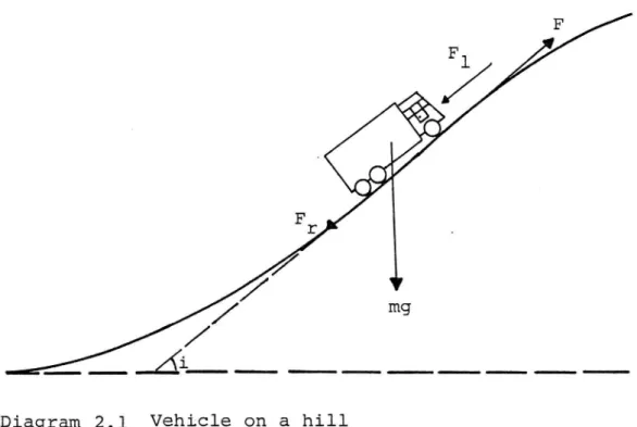
Sub-model describing the effect of hills on the de-sired speed (V,) distribution

The model used is based on the forces which act on a motor vehicle on a hill (see diagram 2.1)

= Tractive force, in N = Air resistance, in N

Rolling resistance, in N = Mass of the vehicle, in kg

= Acceleration of gravity, in m per sec

+-(Q 3 td bj ba |_ .l 11 = Angle of slope

The equation of forces gives

F -

Fl - F, - mgsini = M -r (+ &+ + + k e We We e e e e e e 6 k e k e 6 6 - (1)

where

t

11 the speed of the vehicle, in m per sec

r

1

.

11 _{the time, in sec.}

The tractive force, F, which is developed at the

wheels by the engine can be written

po= E

v

where

P = the power output, in W, developed by the tractive

force

The resistances are dependent on several factors, as

may be seen from the following equations.

The air resistance, Fl' is

_ 2

= a "shape factor" of the vehicle, in kg per m3

Q I

the front surface area of the vehicle, in m2

15

Vr = the relative velocity of the vehicle with refe-rence to the surrounding air, in m per sec, which is approximately equal to the speed of the vehicle, v, in m per sec.

The rolling resistance,

Fr' is

==

i /N

Fr

where

C, = a constant which is dependent on the road surfacing and on the type of tyre.

This equation disregards that component of the

rolling resistance

Fr' which is dependent on the speed.

Finally, the gravitational component may be

approxi-mated by mqsini # mqi.

If the above expressions are substituted in Eg (1)

then we obtain

P

2

,

dv

>

This equation can be written

C, A

dv _ E o 1 2 o f .

Se 20 -- v Cr FÅ u e e e e e e e e e e e e e e e e e k e e e e ( 2)

where P =

å is the used power to weight ratio for the

vehicle.

In the model, every vehicle is assigned a p-value,

which is the maximum used power to weight ratio

In addition it is assumed that the "coefficient of air friction" , ClA is constant for all vehicles

m in a given vehicle class.

Now, in theory, it is possible, for each road block, and for each vehicle, to solve equation (2) numerically to find the maximum possible speed at any point in the block. This speed could be compared with the desired

(V3) speed of the vehicle, and the lower of

the two speeds used.

In practice, however, it would be cumbersome to

rigidly apply the above method, for the repeated

solving of equation (2) is a lengthy process.

A

simplified method is therefore used as follows.

For each road block, and for each vehicle, the

equilibrium speed, Va g is found by substituting

dv _

.

.

.

ax * 0 in equation (2).

If Va > Va i then v is used.

Only if v, © v, is equation

(2) solved numerically.

This speed is then compared with V 3 i and the lower

of the two speeds is used.

The combined model for free-moving vehicles

Diagram 2.2 shows a graph cf typical speed changes

for four free-moving vehicles.

Vehicles A and B are both cars.

A has a higher speed

class than B, but they both have the same p-value.

Vehicles C and D are both lorries.

They both have

the same speed class, but C has a higher p-value than

D .

17

In each case, the solid line shows the speed profile for the vehicle, while the dotted line shows the same profile, but neglecting the effect of hills.

VTI MEDDELANDE 43

Diagram 2.2. Free speed profiles.

km /h Fr ee s p ee d pr of il es 10 0 W i 9 0 - x 8 0 -> myeS t a 70 -6 0 -50 4 4 0 -S p e e d li mi t ( k m / h ) _

I

90

-=

&=

Di

re

ct

io

no

ft

ra

ve

l

m

Ve

rt

ic

al

pr

of

il

e

.4

0

19

THE MODELÅ FOR BOTH FREE-MOVING AND INTERACTING VEHICLES

Interacting Vehicles

A vehicle is interacting if it is either constrained by another vehicle or overtaking another vehicle.

A vehicle ej; is constrained by e; if ej; is travelling at a speed lower than its desired speed because it is following ej. If ej, e7, .... ep are a string of

vehicles such that e; is constrained by ej,j (i=1l,2,.. .. n-1), then the vehicles ej, ©2 r. + ++ - en form a

platoon, and er is the platoon-leader. A platoon may consist of just one vehicle.

Two types of overtaking may be distinguished. If e; is not constrained by ej, so that ej continues to travel at the same speed when it overtakes 23: then the overtaking is called a flying overtaking. If ej does become constrained by ©3, SO that e, eventually has to accelerate in order to overtake © 3 , then the overtaking is called an accelerative overtaking.

The status of a vehicle may be loosely described as its state of constraint and/or overtaking. It is naturally possible for a vehicle to be neither con-strained nor overtaking; it is then free-moving. It is also possible for a vehicle to be both constrained and overtaking. This occurs when a platoon consisting of more than one vehicle overtakes another slower

platoon .

Events

An event for a vehicle is a point in time when that vehicle may change its state of motion.

free-moving vehicle is determined by the road conditions, so that the only event for such a vehicle is the passage of a block limit.

However, when interaction is possible, there are further event types which occur whenever the status of a vehicle may change. (In general, a change in a vehicle's status may involve a change in that vehicle! s state of motion) .

When interaction is possible, an event occurs each time a vehicle passes one of the following points:

(1) -A decision point for flying overtaking

(2) -A decision point for accelerative overtaking

(3) -A point of overtaking (when the overtaking vehicle is at the same distance coordinate as the over-+akaemn vah ic] e '_{ko- Goa T SZ & & 5} V..;J.."-v_4 V/

(4) -A point where an overtaking finishes

(5) -A block limit

These events will be described in section 3.3.

The simulation of interactions between vehicles

Decision Point for _ Elying_Overtaking

Suppose a free-moving vehicle ej is catching up with

a slower vehicle, e At some point, e; must decide

whether or not to

fäying overtake e.

In the

calcu-lation of this point, it is assumed that if ej; rejects

the overtaking opportunity, then it must be able to

decelerate at a fixed rate R, to reach a fixed time

headway T away from 23 i when ej; has attained the speed

of e; .

(R=3 m/sec/sec, and T=1 second)

2 1 | 1 / I I 1 i i 1 | I 1 1 I 1 I | I | SJ Sa + D Sf $f+TVJ

Let (S4, t4) be the decision point.

Let (Sr, tr) be the point when ej has decelerated to the speed, V 3 g of e; .

Let D be the distance headway at time tg.

Then

D + = - Så '

Vi = Vy= Ritz + ta)

% vi 7 % vå

=

- Så)

Hence

D = Tv; + (v; -

V1)2

2R

This distance headway, D, is the maximum at which a

decision on flying overtaking may be made, but there

are occasions when a decision must be made at shorter

notice.

For example, if ej is at the point of

over-taking another vehicle, e,, then e; may make an

immediate decision on flying-overtaking the next

vehicle ahead, if the new headway is less than or

equal to D.

On

If ej; rejects an opportunity to flying-overtake s then e; automatically becomes constrained by ©3. j may then have to make a subsequent decision on whether

to accelerate past ej. (See the following section) .

Decision Point for Accelerative _ Overtaking

If e; is constrained by © 3 , then it may make a decision on whether or not to accelerate past ©; when it next encounters either of the following:

(1) -A block limit where an extra lane (ie. a crawling lane or wide hard shoulder) begins.

(2) -A point of maximum sight distance

In the latter case, the sight distance may be restricted "F"-i

() mara_; 1/mv svl7 m ee Zn fyS4 &

1LL.L....Lj f.).q f Fat Set Fn ..i- ) 1

by the presence of an oncco

and the opportunity to overtake was rejected on that

occasion, then a new decision is made when the last

vehicle in the oncoming platoon has passed.

If e; rejects an opportunity to accelerate past ej,

then further decision points are generated, as described

above, until e; does decide to overtake.

The _Overtaking _ Decision Process

Suppose e; has to decide whether or not to overtake

e; . Let block (i), block (j) be the road blocks currentby

occupied by i, j. Then e; rejects the overtaking

opportunity if any of the following conditions hold:

(R1) e; is itself being overtaken

(R2) e; cannot develop enough power to overtake e..

(This condition can only hold at decision points

for accelerative overtaking)

(R3) There exists a no-overtaking zone in block (i)

(R4) There exists a solid white line in block (i) and

2 3

Now if there exists an extra lane in block (3), then there is a fixed probability (dependent on the type of extra lane, and the vehicle class of

ej) that © wi l l

move over into this lane, to allow ej; to overtake.

Monte Carlo methods are used accordingly to decide

whether e, does in fact move over.

This provides a

further condition for ej rejecting the overtaking

opportunity:

(R5)

There exists a solid white line in block (i)

and there exists an extra lane in block (j),

but ©; does not move into the extra lane

There is one condition which ensures acceptance of the

overtaking opportunity:

(Al )

There exists an extra lane in block (j) and

ej moves into the extra lane.

If none of the conditions (R1I) -> (R5) or (Al) hold, then the outcome of the decision is not certain. Functions have been calibrated, which determine the probability of accepting a gap of given length in order to overtake, in each of 32 different overtaking situations. (See section 6.4) . Monte Carlo methods can therefore be used in order to make the decision.

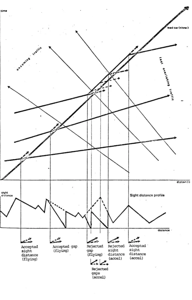
A schematic representation of three fast vehicles overtaking a single slower vehicle is shown in diagram 3.1.

When a vehicle is at the point of overtaking another vehicle, it examines the possibility of flying over-taking the next vehicle ahead (as explained in section 3. 3.1) .

_distar-> sight

distance Sight distance profile

7 ) | , i distance : y = d P d Lat>> Se ULar er

Accepted Accepted gap . Rejected Rejected Agcepted i

sight (flying) gap sight s;ght distance - (flying) distance cålstaåce

(flying) (accel) accel)

les leZ, Rejected gaps

(accel)

25

An overtaking finishes at a fixed time interval u after the point of overtaking. (u = 3, 4, 5, and 6 seconds for overtaking vehicles of classes l to 4 respectively) .

Passage _ a_block_ limit

A vehicle's desired speed may change at the passage of a block limit, and this can affect the interactions involving the vehicle. For instance, at the approach of a hill, an overtaking vehicle may find that it must abort the overtaking because it can no longer develop sufficient power to maintain the required acceleration. A constrained vehicle may become free-moving for the

same reason.

Prediction of events

A vehicle's event-notice contains details of the event currently predicted to take place next, for that

vehicle. The operation of the model relies on the maintainance of an up-to-date list consisting of one event-notice for each vehicle. The simulation pro-cedes by selecting the next predicted event in this list, and examining the consequences of this event. In general, these will entail the updating of both

(&) The current status and state of motion of several vehicles, and

(b) The event-notices of several vehicles

The prediction of events is based on both the current status and state of motion of the vehicles, and the description of the simulation given in section 3.3.

Results

There are two output files which give details of the results of the simulation, and these are described in chapter 5.

27

MODELL INPUTS

Road data

As described in section 2.1, the road to be simulated must be described (in each direction) as a series of homogeneous blocks, each of which has constant road geometry and traffic regulations.

The data required for each road block and in each direction is as follows:

(1 ) Distance - coordinate of start of block (metres) (2) Width (metres)

(3) Radius of Curvature (metres) (4) Speed limit (km/hr)

(5) Slope, n (n per mille)

(6) Overtaking restrictions code (7) Hard shoulder/climbing lane code

Here, item (6), the overtaking restrictions code for block k, pass (k) , is defined as follows:

pass (k) = 0 No restrictions

1 : No overtaking allowed

A further overtaking restriction which can occur is the presence of a solid white line painted down the middle of the road. However, in Sweden, the existence or otherwise of this line is solely

dependent on the speed limit and the sight distance, so this information is not required as separate data.

Item (7), the hard shoulder/climbing lane code for block k, lane (k), is defined as follows:

lane (k) = 0 : Neither climbing lane, nor hard shoulder (i 2 metres) exists

i ; Hard shoulder (i 2 metres) exists 2 ; Climbing lane exists

In addition to the above, the following data have to be specified for each sight-distance maximum or

minimum along the road, in each direction:

(8) Distance-coordinate of the sight-distance maxki-mum/minimum (metres)

(9) Sight distance (metres)

The Swedish National Road Data Bank contains data

items (1) to (7) for most of the Swedish road network. Items (8) and (9) generally have to be collected

specially for a simulation run.

Vehicle Parameters

The two _ modes _ of operation

Individual vehicle parameters can either be obtained with the aid of individual vehicle data, or generated automatically from aggregated vehicle data (and road data) by separate sub-models.

Up to the time of writing, the first mode of operation has been the most commonly used, as some of the sub-models for the automatic generation of vehicle para-meters are still under development.

Section 4.2.2 below describes the individual vehicle parameters required as input into the model. Section 4.2.3 describes how these parameters are obtained from individual vehicle data, and section 4.2.4

describes the sub-model for the automatic generation of vehicle parameters.

29

4.2.2 Description _of parameters

The term "parameters" has been preferred to "data" here, because an individual vehicle (unlike a road!) has characteristics which, though they are required as inputs to the model, cannot realistically be collected as data.

The parameters required for each vehicle are as follows:

(1) Identity number (2) Vehicle class (3) Speed class

(4) Power to Weight Ratio (5) Direction

(6) Initial and final block numbers (7) Initial time coordinate and speed

Here, item (1) is an identifier, items (2) to (4) are vehicle characteristics which have previously been defined and items (5) to (7) specify the boundary conditions necessary to operate the model.

Use of Individual Vehicle Data for the Generation of _ Taramsters_

4 ,. 2.3 1 The Data Collected

Individual vehicle data is collected with the aid of equipment specially designed for this purpose. A brief description of this equipment is given as an appendix to this paper. Using this equipment, in-dividual vehicle data in both directions is collected for any required time period at each of three points along the simulated road - viz. the start, the finish, and a point roughly midway between these. The raw

4 . 2 . 3 . 2

data is processed to produce the following data for each vehicle:

) An identity number ) The vehicle class ) The direction

) The spot-speed (At each of the three points ) The arrival time

:%

which the vehicle passed)

It is possible for no data to be available at one or

two of the three points.

This occurs when the vehicle

enters or leaves the simulated road between the start

and finish points.

It is now clear that parameters (1), (2) , (5) , and

(7) are immediately available from the data collected.

Item (4) is always generated automatically (see section

4.2.4 .4) .

The remaining items are obtained as follows:

Speed Class

This is a measure of how fast the vehicle wishes to

travel, compared with other vehicles on the road, so

the spot-speeds of all vehicles are used as follows:

Firstly, for each of the recorded points, the

distri-bution of observed spot speeds is constructed.

Now

each vehicle belongs to a 4-percentile of the observed

speed

distribution at each of the points where it was

observed.

Let m be the maximum of these 4-percentiles.

Then each vehicle which was free-moving at one or more

of the points is assigned to speed class m.

(Here ,

"free-moving" is defined by specifying some minimum

time headway for free-moving vehicles) .

If no free speeds were recorded for a vehicle, it is

likely that m is too small an estimate for the speed

4 . 2 . 3 . 3

31

class, so instead, the value (m+r) is used, where r is a random number sampled from £O,l,2,3,43

Initial and Final block numbers

Block numbers are recorded for all junctions along the road.

Let A = The starting point of the simulated road, B = The mid point were data was collected. C = The finish point.,

Then a probability distribution is estimated, which assigns to each junction j between A and B, the pro-bability of a vehicle leaving the road at j, given that it left the road between A and B.

Similar distributions are estimated for

(a) Vehicles leaving the road in the stretch BC (b) Vehicles entering the road in the stretch AB (c) Vehicles entering the road in the stretch BC

Now for all vehicles which were not recorded at

either A or C, it is possible to deduce which of the above categories the vehicle belongs to. Hence ini-tial and final block numbers can be assigned to each vehicle by sampling from the appropriate probability distribution.

Automatic _ generation _ of vehicle _ parameters

(It is assumed in the following that the only vehicle data available is the total traffic flow and the

composition of this flow by vehicle class, in each direction) .

4,2 .4.l1 Identity number

This is trivially generated by incrementation each time a vehicle enters the simulation.

4 , 2.4.2 Vehicle Class

A distribution of vehicle classes is supplied by the traffic composition. The vehicle class of an indi-vidual vehicle is obtained by sampling from this distribution.

4.2.4 .3 Speed Class

The following prototype method is currently being used:

(4) For vehicles of class 1, a random sample is taken from i_Kor 1,2,... 143 with probability 0.5

£ 15,16 25 3 with probability 0.5

(b) For vehicles of class 2,3 or 4, a random sample is taken from it 1,2.... 133 with probability 0.95

t 14 ,15,.. 253 with probability 0.05

It can be shown that if the traffic composition is 85% (class 1) and 15% (classes 2,3 and 4), this method assures that the expected number of vehicles in each desired speed class is approximately equal.

4 . 2.4.4 Power to Weight Ratio

A p-value is sampled randomly from the p-distribution relevant to the vehicle's class. (See section 6.3 for a description of the p-distributions) . A check is then made as follows to assure that the vehicle can maintain its basic desired (V) speed, on a flat road, with this p-value.

33

The equation of motion for a vehicle (equation (2) in section 2.5) is

setting

%% = 0 and i = 0, we obtain the following

equation for the equilibrium speed, v,, for the

vehicle with p-value p.

_C1lA

vå + Cr Ve " P = 0

m

This may be solved numerically, for v,.

Then if v,

is greater than the desired (V) speed for the

vehicle, the condition is satisfied.

Otherwise, new

p-values are sampled until the condition is satisfied.

Direction

This is trivially generated.

Vehicle data is generated

corresponding to the traffic flow in each direction.

Initial and Final Block Numbers

It is assumed that every vehicle enters the road at

the first block and leaves it at the last block.

Initial Time Coordinate and Speed

Currently, the sub-model to generate initial time

coordinates requires additional input data - viz. the

proportion of free vehicles, platoon leaders, and

vehicles following in platoons, each by vehicle type.

This enables platoon lengths to be sampled.

Free

vehicles are then given a time headway sampled from a

negative exponential distribution, with a shift of 3

seconds (this being the assumed minimum free headway) .

Constrained vehicles are given a fixed time headway

of 1.2 seconds.

Free vehicles are assigned an initial speed equal to their desired (V;) speed. Constrained vehicles are given the same initial speed as the platoon leader.

There is a facility which enables the flow to increase (or decrease) at a constant rate as the simulation procedes.

Work is in hand firstly to determine the sensitivity of the model to the initial time headway distribution and secondly to produce a general distribution of platoon sizes.

35

MODEL OUTPUTS

Summary of results

At the conclusion of each simulation run, the following summary of results is printed (for each direction, both by vehicle class, and for all

vehicles) .

(a) Total number of vehicles simulated. (b) Total vehicle-kilometres simulated.

(c) Mean journey time along the whole simulated road. (d) Mean journey speed along the whole simulated road. (e) Total number of overtaking vehicles.

(f) Total number of vehicles overtaken.

There are also two output files produced which may be used to analyse the simulation in more depth. These are described in sections 5.2 and 5.3.

File of Simulated Vehicle Movements

One output file produced by the model gives a

summary of each vehicle'"s simulated movement along the road. Thus there is a record for each vehicle, in each direction, giving

(a) Identity number, i (b) Vehicle Class of i

(c) Time coordinates of i at A, B, C. (d) Spot speeds of i at A, B, C.

(e) Journey speeds of i in sections AB, BC, AC. (f) Time headways of i at A, B, C.

(g) Identifiers of vehicles immediately in front of i at A, B, C.

(h) Identifiers of vehicles immediately behind i at A, B; C.

(i) No. of overtakings by i, for each vehicle class, in sections AB, BC.

(j) No. of times i was overtaken, by each vehicle class, in sections AB, BC.

This file is in exactly the same format as that pro-duced from individual vehicle data (if the latter was collected), thus facilitating the comparison of observed and simulated vehicle movements.

If desired, the file may be simply listed, but it is also possible to analyse it as follows:

(1) For any class of vehicle, and for any stretch of road (AB, BC or AC) , a histogram of travel times may be constructed, and the total number of observations, mean, and standard deviation printed.

(2) For any class of vehicle, and for any station (A, B or C), a histogram of time headways may be constructed, and the total number of obser-vations, mean, and standard deviation printed.

(3) For any class of vehicle, and for any station (A, B or C) , a histogram of spot speeds may be constructed, and the total number of observa-tions, mean, and standard deviation printed.

(4) For any stretch of road (AB, BC or AC) , a table of overtakings (by class of overtaking vehicle, and class of overtaken vehicle) may be construc-ted.

These analyses may be made for any desired interval (s) of simulated time.

NB: In the above, A, C, and B are the three points described in section 4.2.3.1; viz. the two end points of the road, and a mid-point.

37

File of events

This output file contains a record for each event in the simulation run. This record specifies the time of the event, the primary vehicle in the event, the event type, and a considerable amount of further informa-tion concerning the state of the vehicles on the road when the event took place.

The records of the file are ordered by increasing event times, but if desired, just the events relating to a single vehicle may be listed.

This file may also be used to produce the following plots:

(1) -A plot showing the percentage of

(å) Free Vehicles

(p) Constrained Vehicles (c) Overtaking Vehicles

at any given road block.

See diagram 5.1 for an example of this plot. The curves below and above the centre line apply to the traffic in directions 1 and 2 respectively. Thus, in direction 1, at block limit x, there are p* of free-moving vehicles, q% of constrained vehicles, and r? of overtaking vehicles.

(2) -A plot showing the function

h(k)= FIK) -te (k) x (k)

at any given road block, k. where

x (k) = the length of block k

t(k) = the mean simulated journey time within block k

Ef(k) = the mean simulated journey time within block k, assuming that every vehicle is free-moving, throughout the simulation.

h(k) is the mean delay (per vehicle, per unit dis-tance) caused by congestion at road block k. Thus, this plot may be used as an indication of the

stretches along a road which would benefit most from improvement.

Diagram 5.2 shows h(k) plotted for (A) an existing road, and

(B) a proposed improvement.

As in diagram 5.1, the curves for the two directions are separated by the centre line.

10 0 led i#* Å J *.i å e" . 3 &, f* i i 5 0 1 5 0 -D i r e ct i o n 2 n -D i r e c t i o n 1 s e -r 39 D i a g r a m 5 . 1 . T r a f f i c s t a t u s .

b--D i a g r a m 5 . 2 . D e l a y s c a u s e d b y c o n g e s t i o n . x ___=-see % 0003 angr me D i r e c t . i o n 2 -o r vä rn / " f 2 * er e D A r e c t f o n _ '

x/

Vx

/

s%

ka

-4 1

CAL

The basic desired speed (V) distribution

This distribution is described in section 2.1.

Data for the calibration was collected between 1963 and 1967. Vehicles' spot speeds were measured at several points along different roads. The quality of each road was very good, with respect to road width and both vertical and horizontal alignment, and there was no speed limit at any of the points. Furthermore, the traffic flow along each road was low, so that

nearly all the vehicles were free-moving.

The basic desired speed of each vehicle (provided it was at at least one of the points) was taken to be the highest spot-speed recorded for the vehicle. Vehicles which were constrained at every recorded point were ignored, but this occurred suffi-ciently rarely for it to have very little effect on the resulting distribution.

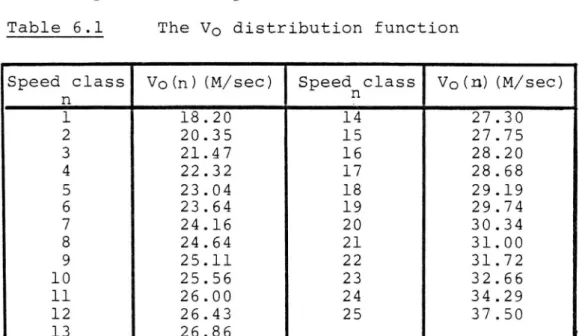
The calibrated V distribution function is listed in table 6.1 and depicted in diagram 6.1 (Each speed class represents a 4-percentile of the distribution) .

Table 6. l The V distribution function

Speed class| Von) (M/sec)

Speednclass

Vo (n) (M/sec)

n

i

1

18.20

14

27.30

2

20 . 35

15

27 ,. 75

3

21 . 4 7

16

28 . 20

4

22 . 3 2

17

28 . 68

5

23 . 0 4

18

29 . 19

6

23 . 6 4

19

29 . 7 4

7

24 . 16

20

30 . 34

8

24 . 6 4

21

31 . 00

9

25 . ll

22

31 . 72

10

235,56

23

32.66

11

26 . 00

2 4

34 . 29

1 2

26 . 43

25

37 . 50

13

26 . 8 6

Qmulative Percentage 100 =75 50 -26 4 Diagram 6 .l.

VO distribution.

30

4 3

Sub-models describing the effect of road width, bends, and speed limits on the basic desired speed distribu-tion

These sub-models are described in section 2.2.

The parameters which required calibration are tabula-ted in table 6.2.

Table 6.2 Calibration parameters

Factor Median model Q model

Road width:

(a) With hard shoulder g(x) (x4*©2.5)

41, %& 1 (b) Without hard shoulder|a

Bends b 42, 42

Speed limits c ,d 43, 93

Data used for these calibrations was collected between 1970 and 1972.

The theoretical approach to these calibrations was as follows:

For each of the three factors i, and for each measure j of i, two speed distributions are measured (using a fixed sample of free-moving traffic):

(å) A distribution of basic desired speeds

(b) A distribution of speeds under the influence of measure j of factor i.

These observed distributions enable the above para-meters to be calibrated.

In practice the above approach was not always possible because it was difficult to find roads which isolated

first. This was used in order to isolate the effect of road width and calibrate the submodel for the lat-ter. Finally, both these sub-models were used in order to isolate the effect of bends, and calibrate that sub-model.

The values obtained for the parameters listed in table 6.2 are tabulated in table 6.3.

Table 6.3 Parameter values

Median model

" Q model

Parameteri

Value

Parameter!

Value

g (0.0)

1.78

[1

g (0.5)

1 . 40

g (l. 0)

1 . 01L

dj;

0 . 5

g (1.5)

0 . 63

o

&]

1.0

g (2.0)

0 . 28

g (2.5)

0 . 00

a

0.042

11)

b

0 . 15

The distribution (p) of used power to weight ratios

The sub-model which uses this distribution is described in sections 2.5, and the sampling procedure used to assign a p-value to a given vehicle is described in section 4.2.4. 4.

It was decided that separate p-distributions should apply to vehicles of different vehicle classes, since vehicle class is quite clearly a major determining

4 5

factor for power to weight ratios.

However, there was no data available with which to measure the p-distributions directly, so they were calibrated instead, using a derivation (described be-low) from the sub-model described in section 2.5.

The basic equation (2) derived in section 2.5 is

ät v

Integration of this yields

V £ t CiA t t

J

vdv = J pdt

J

71-1 vVdt -J Crvdt

J

givdt

dv

_{- P _}

CjiA

.

Vo 0 0 0 0

where

Va is the speed when t = o and v is the speed at time . This simplifies to t v n cia (* s

S

pdt =j

vdv + gj. dh + _å J.

vZds + CI).

ds

O

Va

O

O

O

(See diagram 6.2)

Diagram 6.2

VTI MEDDELANDE 43

Thus,

= v2 - va? gh 1 [* 2 CyS

P = + iF + i (*)] vide + *F*

# 0

2» L

where p =

Ek[

pdt

is the mean used power to weight

0

ratio for the vehicle in the time (0,t) .

Now the following assumptions are made:

(å)

p = p, a constant for the vehicle under

conside-ration.

(b)

The "coefficient of air friction",

s _{2 m. P}3

(C)] VdSN t Z

0

Hence the following equation is obtained:

2 2 3

- - 9h , S CrS V TV o f,

P 21 * rt * hå ) t ... (1)

Now, in 1969, the following data was obtained for a sample of traffic on a steep hill.

(i) The journey time, t, from a point at the bottom to a point at the top of the hill.

(ii) The spot speeds vp and v, at the bottom and the top of the hill.

The distance, s, between the two points, and the diffe-rence in height, h, were also measured, and the ve-hicle class of each veve-hicle was recorded.

This data was used, together with equation (1) to ob-tain the required p-distribution for each of the four vehicle classes.

47

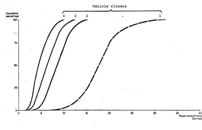
These distributions are listed in table 6.4, and de-picted in diagram 6.3.

Table 6.4 p-distribution functions for each vehicle class

p (W/kg) % (Vehicle (Vehicle % (Vehicle |% (Vehicle class 1) class 2) class 3) class 4)

1 0 ..0 0 . 0 0 . 0 0 . 0 2 0 - 0 0 . 0 0 . 0 0 . 4 3 0 . 0 0 . 0 2, 5 13 . 0 4 0 . 0 4 . 5 10,1 43 , 3 5 0 . 0 6 . 0 23 , 5 59 , 3 6 0 . 4 15. 6 39. 5 68 . 5 7 0 . 4 26 -. 6 57 . 2 83 . 2 8 1 . 0 39. 7 71. 4 93 . 3 9 2 ..] 48 . 7 85. 7 96 . 7 10 4 , 2 6 4 . 8 91. 6 99. 2 11 4 . 6 78 . 4 96. 7 99. 6 1 2 8 . l 85. 8 100 - 0 100 - 0 13 $ , 8 93. 0 14 13. 7 97 -. 0 15 22 . 5 99 .- 0 16 30 -. 2 99 - 0 17 40 . 3 99. 5 18 50. 2 99. 5 19 60 . 4 100 - 0 20 71. 2 21 79 . 3 22 86. 4 23 89 - 6 2 4 91. 2 25 91. 6 26 95. 2 27 96 . l 28 96 - 1 29 96. l 30 97 - 9 31 98 . 2 32 98 . 6 EX 98 . 6 3 4 98 - 6 35 99 . 3 36 99 . 3 37 99 - 3 38 100 - 0 e n e

Vehicle classes Cumulative # , percentage 4 3 2 + 1 100- s aren. agg

fffff'

75-

/

9

₀

₅

omer".

₁₀

₁₉

₂₀

_{000 %s}

₃₀

_'

_as

₄₀

Powertoweightratio

4 9

Probabilities of Gap Acceptance

The probability of accepting a gap of given length in order to overtake is required by the model in each of 32 different overtaking situations; viz

Overtaking Manoeuvre - (1) flying

- (2) accelerative Limitation - (1) oncoming car

- (2) sight distance Vehicle Overtaken -(1) vehicle class 1,

travelling at a speed £ 72 km/hr - (2) vehicle class 1, travelling at a speed > 72 km/hr - (3) vehicle class 2 - (4) vehicle class 3 or 4 Road width - (1) there exists a hard

shoulder > 2 m or a climbing lane

- (2) neither of these exists

The studies which have been used in order to estimate these gap acceptance relationships were conducted in 1967 and 1968 by Åhman.

Using a test vehicle as the overtaken vehicle (in each of the 32 overtaking situations) , observations were made of the number of gaps accepted and rejected. The number of acceptances and rejections were plotted

against the gap distance and from this data, robust relationships (giving the probability of a given gap being accepted) were derived. (See diagram 6.4 for an example of this) .

All the relationships derived were of the form

0 (x © s;)

p(x) = a(x-s1)/(s2-s;) (s] IxASs>)

a (Sx)

where x is the gap distance and a, sj, s3 are calibra-tion constants.

Diagram 6.4.

VTI MEDDELANDE 43

Overtaking gap acceptance relationship.

NO of ga ps rej ect ed 60 Pr ob ab $t yo fa ga p be in ga cc ep te d 50 10 -40 Sig ht os tanc er estruc ied L& ud car 60 km /t i Accele ratedo ver lak ing t -8 Ro ad wid th m 1 Sh oulder wd in 1= Im 30 20 ga pd is ta nc e( m.) 20 30 40 50 " 0 y NO of gaps ac ce pt ed 0 20 0 40 0 60 0 80 0 n 10 00 , i G a p di st an ce .m et re s a . O b s e r v e d d a t a 0 b . R e l a t i o n s h i p

51

The values of a, Sj» Sx in each of the 32 overtaking situations are tabulated in table 6.5. It should be noted that ag l in every case. In other words, no matter how favourable the overtaking situation may be,

there is always some proportion of drivers who will not overtake.

Table 6.5 Gap acceptance relationships

OVERTAKTNG LTMTITATION VEHICLE ROAD a i s2 MANOEUVRE * OVERTAKEN WIDTE [(Probability)! (Metres) (Metres)

2 2 1 2 . 60 50 500 1 2 1 2 95 -150 400 2 1 1 2 . 50 150 1100 1 1 1 2 . 80 50 500 2 2 1 . 1 . 90 50 700 i 1 2 M 1 95 , -150 400 i 2 1 1 1 , 54 50 1250 1 1 1 1 ,85 -150 500 2 2 2 2 . 50 100 700 1 2 2 2 95 -150 500 2 1 2 2 50 150 1100 1 - 1 2 2 75 50 550 2 2 2 1 70 100 800 H 2 2 _ 1 95 -150 500 2 1 2 1 , 50 50 1250 1 1 2 1 .80 -100 500 3 2 3 2 - 70 100 800 1 2 3 2 . 60 100 700 2 1 3 2 30 300 1300 1 1 3 2 55 150 900 2 2 3 1 75 100 600 1 2 3 1 . 70 0 700 2 1 -= 3 L . 60 150 1000 1 1 3 1 70 0 700 2 2 4 2 70 100 800 1 2 4 - 2 . 60 100 700 2 1 4 2 . 20 350 1100 1 1 4 - 2 | 30 500 1300 3 2 4 1 . 60 100 700 1 2 4 1 ,.30 400 1300 2 1 4 1 - 20 200 1000 1 1 4 L . 30 500 1300

VAÄLTDATILION

General philosophy

In an ideal world, separate models would be designed to meet the needs of each study, and the criteria for the successful validation of a model whould be depen-dent on the purpose of the study.

In practice, however, it is often convenient to use the same basic model form in several separate areas of application, and this has been the case with the model described in this paper.

Thus, validation of the model is necessary in two different situations. The first of these is prior to a specific application of the model, when criteria for successful validation may be clearly defined. Validation exercises like this were conducted prior

to the use of the model in the two major studies de-scribed in chapter 8.

The second type of validation envisages a more general situation (for instance, the development of flexible road design standards) where the model is used with a variety of input data, and any of the model outputs may be required.

It is this second, rather badly defined, type of vali-dation which is described in this chapter. The work involved in this exercise is only partially completed, so that only a broad indication is given of the results obtained so far.

Techniques

53

complexity, by taking into account the following fac-tors:

(a) Road width, bends, and speed limits. (b) The factors in (a) plus hills.

(c) The factors in (b) plus interactions between vehicles.

The complete validation exercise which is being under-taken involves the validation of the model at each of these three levels of complexity, starting with

(4) , and finishing with (c), which is the whole beha-vioural model. The techniques used at each stage have been broadly similar, and are described in the following paragraphs.

First, stretches of road were chosen, which varied with respect to the factors being considered. In stages

(4) and (b), a low traffic flow was required, so as to obtain a high proportion of free-moving vehicles. DTA-2 equipment (see appendix) was used to collect data at (at least) three points along each road.

Now the object of the present exercise was to vali-date the behavioural model, rather than the distribu-tions and sub-models which are used to assign input vehicle parameters to individual vehicles. Thus, in general, the data relating to one part of each road was used to give as good as estimate as possible of the vehicle parameters required as input to the model. Then, the data for the remainder of the road was used for the validation of the model. Thus, for example, in stage (b), p-values were assigned to each vehicle as described in section 6.3, and at all stages, a similar method to that described in section 4.2.3 .2 was used to assign a speed class to each vehicle.

G)

At each stage, the main criterion for successful vali-dation was a good fit of the simulated distribution of journey speeds to the observed distribution. In the validation of the whole behavioural model (stage

(c)), other important criteria were good fits of both the number of overtakings, and the final time headway distribution, to the observed data.

It should be mentioned here that the observed data (eg. journey speeds) are not independent of each other when interaction between vehicles has taken place, and this produces problems when assessing goodness-of-fit. A detailed analysis of these problems is, however

outside the scope of this paper.

"1

u slik jön 4 sa Å sa se njacg oa 7 v Te. iLmiÅNary Yresuits

The results of stage (a) of the validation exercise were broadly satisfactory, with simulated journey speed distributions closely fitting the observed data.

Stage (b) at first produced unsatisfactory results, but these were traced to a bad approximation in the solution of equation (2) (section 2.5) . An improved method for the solution of this equation led to sig-nificantly better results.

Stage (c) is still in progress; preliminary results indicate a satisfactory fit of journey speeds, but too many simulated overtakings. It is felt that this could be the result of too many overtakings within platoons, as this would not have a marked effect on the simulated journey speeds. Work is in hand to correct this fault.

55

APPLILCATIONS

Crawling Lane Study

The first major application of the model was to evaluate different stategies for building crawling lanes up a hill. For this study, particular attention was paid to two different types of lorry (those

carrying timber and cement), for these were major users of the road, and it was considered that they were responsible for a lot of the delays which could be avoided with the construction of a crawling lane. Thus, p-values for these two classes of vehicle were

specially calculated, and estimates were made of their frequencies in the traffic flow.

The first stage of the study was to simulate free moving vehicles travelling up the hill.

Diagram 8.1 shows the vertical alignment of the hill, together with the free speed profiles for both a

timber and a cement carrying lorry. The top profile is the desired speed profile for both these lorries

(neglecting the effect of hills). It is assumed in this diagram that both lorries have the same speed class.

It may be seen from diagram 8.1 that the initial steep part of the hill (AB) has a lasting effect on the free speeds of these lorries. In fact there are 3 severe minima in the free speed profiles, at Mz and M3 as well

as at Mj. This indicated that it might be beneficial to build a crawling lane up the whole hill (from A to C) . This strategy was contrary to the design standards, which specified a crawling lane only for the steepest section of the hill, AB.

Speed (km/h) 70 60 50 i : i fmm ed emeak ra mv ekm mee isene mse 3 40 30

Height (Metres) »» [_ ai pe.

/ free Speed Profiles ,!|: CE -Är_{- >-p--}- ids

1 f 1 äver samme ers

ort "| Desired speed profile

_ i j e -w i

sött ef r se fen see dee -J- -a

+ 40 1 - " i ; j 104, | ' I )

[lo sar Sö n sv desse t ' vel. snönsa hon :a ansen o -..._,....l sen. Mus © Ge avs f .'_...Å 4 sn los fs t '_

» 7 + Ml I _] .I L t + . I + v 2 LL 7 : -- Height Profile - |- B i 7-1" " t " ' . i -Ja LL 77) T t i . -. ; ) ! . I _ Le. L] dh TX 1$

-dne Joe See -+p- 0 s- $ ... m -- +-1+--1--4+- L..

| ! 1 ! 20 . 1 28 [ 204 '

- T 3 amnev ang kv b seee!- mom dm e sn i + assar sksee v ks :-, .. +sams een idsem 1 .:. ske ; :.i sa D sme

T e c k e peer r e d i i

" 3000 ; ; 3 3500 © =

Diagram 8.1.

1590

Crawling Lane Study:

p% .Di'stance (Metres

Height profile and resulting free speed profiles for two types of vehicle.

Diagram 8.2. VTI MEDDELANDE 43 l n gcl im bi ng l a n e F X 2 0 % l o r r i e s X s s e : r ka 15 % lo rr ie s sh or t å cl im bi ng la ne no clim bi ng la ne *Se s ke r , x o % f e s s > X 20 % lo rr le s 0 sc n s s . / s a . " .. N N x , , , X o ; & % N %. > h r e > 1 5 % l o r r i e s 2 0 % l o r r i e s _ _ _ |" > > . s a " -A 5 7 total flow.

mean journey speeds

as a function of

Crawling lane study:

_ 7 0 1 5 % lo r r i e s 6 0 -' 7 5 0 1 0 0 0 » I 7 v e h i c l e s / h r "

In the second stage of the study, the complete model was used to simulate the following situations:

(a) The existing road with no improvements (b) A crawling lane up section AB

(c) A crawling lane up section AC

In these simulations, substantial stretches of the road beyond A and C were included, so as to observe the after-effects of each situation on traffic nego-tiating the hill. Varying assumptions of traffic flow and composition were made.

Diagram 8.2 shows the speed/flow curves produced. (Here, the speeds are mean speeds for all vehicles, along

the whole simulated road). Finally, the journey times produced by the model were input into economic evalua-tions of strategies (b) and (c) .

Study of improvements to a major trunk road

In this study, three strategies for the improvement of a major trunk road were to be considered. Thus, the model was used to simulate the following situations:

(a) The existing road with no improvements (b) Minor improvements to the existing road (c) Major improvements to the existing road (d) A new "motor traffic road"

Each of the strategies (b) and (c) involved improve-ments to the road width, vertical alignment, and sight distance profile. The new road in strategy (d) also had increased speed limits. For the simulation of strategy (d), an estimate had to be made of the slit in traffic between the old and new roads.

The traffic flow simulated was that predicted on an annual average day in 1985. This was obtained from the

59

observed 1975 flow, using growth factor techniques.

This study featured the use of the plots of delays due to congestion, described in section 5.3. These were used as a means of indicating improvements which could be made to the strategies being evaluated.

The total simulated journey times in each situation were used as inputs into economic evaluations of

strategies (b), (c) and (d). For this purpose, esti-mates of the following parameters were also obtained

from other sources:

(i) Total predicted accidents (for strategies (a) -> (d) )

(ii) Vehicle operating costs (for strategies (a) -> (d))

(iii) Maintenance costs (for strategies (a) -> (d))

(iv) Construction costs (for strategies (b) -> (d))

The first year rate of return was used to compare strategies (b), (c), and (d).

Future applications

The model has great potential for application in many areas of road planning. Someexamples are given below.

(4) The _development of _ flexible _ road _ design standards The model could be used in order to develop

design standards which reflect the interacting effects of road width, bendas, hills, traffic flow etc. These would represent an improvement on rules which can never be universally applicable.

(b) The development of an accident prediction _model It is felt that traffic status may be an

important parameter in the prediction of accident rates. The plots of traffic status (described in section 5.3) will be useful in this area of development.

The Department of Transport (U.K.) require a simulation model as an aid to the evaluation of very minor improvements to rural roads. To this end, a working collaboration has started between the Swedish and British authorities, which, it is hoped, will lead to the model being adanted for use in the U.K.

6 1.

APPENDIX

MEASUREMENT OF INDIVIDUAL VEHICLE DATA USING DTA-2 EQULPMENT

Description of the DTA-2

The DTA-2 (Differential Traffic Analyser, Mark 2) has been specially designed for the collection of indi-vidual vehicle data. Three rubber tubes A, B and C

(each 15 mm in diameter) are stretched across the road, at a distance of 1.65 m apart from each other. These tubes are connected to the main DTA-2 apparatus which is contained in a box and located at the side of the road. Also connected to this apparatus is a camera which is focused on the road in the region of the rubber tubes. (See diagram A.l)

Diagram A. l

A B C '

nen» d gens. &." SSR

k V 22 0 S, s V & x kn. 3 Camera DTA2! y a ( 3 C B _ 09 o , Q a 2 3 © k E r E F p a " +. 2 % vn £ v ma + hda 1

Located in the DTA-2 box are a paper-tape-punch, and a micro-processor. The latter includes a quartz

crystal, which emits pulses of a known frequency. The apparatus is powered by means of two 12 V batteries.

The first use of the crystal is to generate a time-keeping register with units of 0.6 seconds. This register runs from 0 to 64 units, and every 64 units

(38.6 seconds) the register is zeroised and a time-keeping record is punched onto the paper tape.

Now when a vehicle's front axle first crosses tube A (or tube C), it produces a pneumatic pulse in the tube, which is transformed into an electronic signal, and recorded.

At this stage, the current time is recorded using the time-keeping register described above. In addition, a new register,; which can record time in units as small as 0.417 milliseconds, is activated. When the front axle crosses tube B, this register stops, and the time is recorded.

Finally, the order in which the tubes A, B, and C are crossed by the axles of the vehicle is recorded. It is assumed that the maximum vehicle length is 25

metres, so that a time period can be calculated, during which all axle crossings are assumed to be caused by the same vehicle.

Thus, each time a vehicle crosses the three tubes, a record is punched onto paper tape, showing

(i) The time at the first crossing of a tube (in units of 0.6 seconds)

(ii) The time taken for the front axle to travel the 1.65 metres to tube B.

6 3

In addition, the camera connected to the DTA-2 is pro-grammed to take a photograph each time a vehicle

crosses the tubes. Thus, for every vehicle crossing the tubes, data is obtained both in the form of a paper tape record and a photograph.

Use of the DTA-2

The DTA-2 is used to measure vehicle data in both directions and (usually) at three points along the road.

If the traffic flow is low, it is sufficient to use one DTA-2 to measure data for traffic in both direc-tions. However, as the flow increases, there becomes more danger of oncoming vehicles meeting at the point where the DTA-2 is situated, and this produces a bad data record. Thus it is more satisfactory to use two DTA-2's at each point where data is to be collec-ted (see diagram A .2) .

Diagram A. 2

___ _i u u P

G] m

Data Processing

The punched tape records must be transformed into the format required as input to the simulation,

vi z:

An identity number The vehicle class (a)

(b)

(c) The direction (d)

(e)

The spot-speed (At each of the three sta-The arrival time tlons which the vehicle

passed)

(a) At every station, each vehicle is given a reference number. Then, by comparing the photographs taken at each station, the three sets of data for each vehicle can be correlated. A unique identity number can then be assigned to each vehicle.

(b) The number of axle-crossings in the axle-crossing pattern naturally identifies the number of axles. In addition, the distance (1.65 metres) which separates the tubes from each other is so chosen that the axle-crossing pattern uniquely deter-mines the vehicle class.

(C) The first tube which was crossed identifies the direction.

(d) The time taken for the front axle to travel the 1.65 metres to tube B gives an indirect measure-ment of the spot speed.

(e) The arrival time is directly measured.

It is, of course, also necessary to test the punched tape data records for noise. For instance, one ve-hicle following another very closely may be mistaken for a multi-axle lorry, and occasionally, a reverbe-ration in a tube may produce a pulse without any