Copyright © IEEE.
Citation for the published paper:
This material is posted here with permission of the IEEE. Such permission of the IEEE does
not in any way imply IEEE endorsement of any of BTH's products or services Internal or
personal use of this material is permitted. However, permission to reprint/republish this
material for advertising or promotional purposes or for creating new collective works for
resale or redistribution must be obtained from the IEEE by sending a blank email message to
pubs-permissions@ieee.org.
By choosing to view this document, you agree to all provisions of the copyright laws
protecting it.
2011
CudaRF: A CUDA-based Implementation of Random Forests
Håkan Grahn, Niklas Lavesson, Mikael Hellborg Lapajne, Daniel Slat
9th ACS/IEEE Int'l Conference on Computer Systems And Applications (AICCSA 2011)
CudaRF: A CUDA-based Implementation of
Random Forests
Håkan Grahn, Niklas Lavesson, Mikael Hellborg Lapajne, and Daniel Slat
School of Computing Blekinge Institute of Technology
SE-371 39 Karlskrona, Sweden Hakan.Grahn@bth.se, Niklas.Lavesson@bth.se
Abstract—Machine learning algorithms are frequently applied in data mining applications. Many of the tasks in this domain concern high-dimensional data. Consequently, these tasks are of-ten complex and computationally expensive. This paper presents a GPU-based parallel implementation of the Random Forests algorithm. In contrast to previous work, the proposed algorithm is based on the compute unified device architecture (CUDA). An experimental comparison between the CUDA-based algorithm (CudaRF), and state-of-the-art Random Forests algorithms (Fas-tRF and LibRF) shows that CudaRF outperforms both Fas(Fas-tRF and LibRF for the studied classification task.
Index Terms—Random forests, Machine learning, Parallel computing, Graphics processing units, GPGPU
I. INTRODUCTION
Machine learning (ML) algorithms are frequently applied in data mining and knowledge discovery. The process of identi-fying patterns in high-dimensional data is often complex and computationally expensive, which result in a demand for high performance computing platforms. Random Forests (RF) [1] has been proven to be a competitive algorithm regarding both computation time and classification performance. Further, the RF algorithm is a suitable candidate for parallelization.
Graphics processors (GPUs) are today extensively employed for non-graphics applications, and the area is often referred to as General-purpose computing on graphics processing units, GPGPU [2], [3]. Initially, GPGPU programming was carried out using shader languages such as HLSL, GLSL, or Cg. However, there was no easy way to get closer control over the program execution on the GPU. The compute unified device architecture (CUDA) is an application programming interface (API) extension to the C programming language, and contains a specific instruction set architecture for access to the parallel compute engine in the GPU. Using CUDA, it is possible to write (C-like) code for the GPU, where selected segments of a program are executed on the GPU while other segments are executed on the CPU.
Several machine learning algorithms have been successfully implemented on GPUs, e.g., neural networks [4], support vector machines [5], and the Spectral clustering algorithm [6]. However, it has also been noted on multiple occasions that decision tree-based algorithms may be difficult to optimize for GPU-based execution. To our knowledge, GPU-based Random Forests have only been investigated in one previous study [7],
where the RF implementation was done using Direct3D and the high level shader language (HLSL).
In this paper, we present a parallel CUDA-based imple-mentation of the Random Forests algorithm. The algorithm is experimentally evaluated on a NVIDIA GT220 graphics card with 48 CUDA cores and 1 GB of memory. The perfor-mance is compared with two state-of-the-art implementations of Random Forests: LibRF [8] and FastRF in Weka [9]. Our results show that the CUDA implementation is approximately 30 times faster than FastRF and 50 times faster than LibRF for 128 trees and above.
The rest of the paper is organized as follows. Section II presents the random forests algorithm, and Section III presents CUDA and the GPU architecture. Our CUDA implementation of Random Forests is presented in Section IV. The experimen-tal methology is described in Section V, while the results are presented in Section VI. Finally, we conclude our findings in Section VII.
II. RANDOMFORESTS
The concept of Random Forests (RF) was first introduced by Leo Breiman [1]. It is an ensemble classifier consisting of decision trees. The idea behind Random Forests is to build many decision trees from the same data set using bootstrapping and randomly sampled variables to create trees with variation. The bootstrapping generates new data sets for each tree by sampling examples from the training data uniformly and with replacement. These bootstraps are then used for constructing the trees which are then combined in to a forest. This has proven to be effective for large data sets with missing attributes values [1].
Each tree is constructed by the principle of divide-and-conquer. Starting at the root node the problem is recursively broken down into sub-problems. The training instances are thus divided into subsets based on their attribute values. To decide which attribute is the best to split upon in a node, k attributes are sampled randomly for investigation. The attribute that is considered as the best among these candidates is chosen as split attribute. The benefit of splitting on a certain attribute is decided by the information gain, which represents how good an attribute can separate the training instances according to their target attribute. As long as splitting gives a positive information gain, the process is repeated. If a node is not
split it becomes a leaf node, and is given the class attribute that is the most common occurring among the instances that fall under this node. Each tree is grown to the largest extent possible, and there is no pruning.
When performing classifications, the input query instances traverse each tree which then casts its vote for a class and the RF considers the class with the most votes as the answer to a classification query.
There are two main parameters that can be adjusted when training the RF algorithm. First, the number of trees can be set by the user, and second, there is the k value, i.e., the number of attributes to consider in each split. These parameters can be tuned to optimize classification performance for the problem at hand. The random forest error rate depends on two things [1]:
• The correlation between any two trees in the forest. Increasing the correlation increases the forest error rate.
• The strength of each individual tree in the forest. A tree with a low error rate is a strong classifier. Increasing the strength of the individual trees decreases the forest error rate.
Reducing k reduces both the correlation and the strength. Increasing it increases both. Somewhere in between is an optimal range of k. By watching the classification accuracy for different settings a good value of k can be found.
Creating a large number of decision trees sequentially is ineffective when they are built independently of each other. This is also true for the classification (voting) part where each tree votes sequentially. Since the trees in the forest are independently built both the training and the voting part of the RF algorithm can be implemented for parallel execution. An RF implementation working in this way would have potential for great performance gains when the number of trees in the forest is large. Of course the same goes the other way; if the number of trees in the forest is small it may be an ineffective approach.
III. CUDAANDGPU ARCHITECTURE
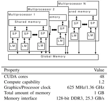
The general architecture for the NVIDIA GPUs that sup-ports CUDA is shown at the top of Fig. 1. The GPU has a num-ber of CUDA cores, a.k.a. shader processors (SP). Each SP has a large number of registers and a private local memory (LM). Eight SPs together form a streaming multiprocessor (SM). Each SM also contains a specific memory region that is shared among the SPs within the same SM. Thread synchronization through the shared memory is only supported between threads running on the same SM. The GPU is then built by combining a number of SMs. The graphics card also contains a number of additional memories that are accessible from all SPs, i.e., the global (often refer to as the graphics memory), the texture, and constant memories. The GPU used for algorithm development and experimental evaluation in the presented study is the Nvidia GT220. The relevant characteristics of this particular GPU is described at the bottom of Fig. 1. In order to utilize the GPU for computation, all data must be transferred from the host memory to the GPU memory, thus the bus bandwidth
S h a r e d m e m o r y S P L M S P L M S P L M M u l t i p r o c e s s o r N S h a r e d m e m o r y S P L M S P L M S P L M M u l t i p r o c e s s o r 2 S h a r e d m e m o r y S P L M S P L M S P L M M u l t i p r o c e s s o r 1 G l o b a l M e m o r y Property Value CUDA cores 48 Compute capability 1.2 Graphics/Processor clock 625 MHz/1.36 GHz
Total amount of memory 1 GB
Memory interface 128-bit DDR3, 25.3 GB/s
Fig. 1. The GPU architecture assumed by CUDA (upper), and the main characteristics for the NVIDIA GeForce GT220 graphics card (lower).
and latency between the CPU and the GPU may become a bottleneck.
A CUDA program consists of two types of code: sequential code executed on the host CPU and CUDA functions, or ’Kernels’, launched from the host and executed in parallel on the GPU. Before a kernel is launched, the required data (e.g., arrays) must have been transferred from the host memory to the device memory, which can be a bottleneck [10]. When data is placed in the GPU, the CUDA kernel is launched in a similar way as calling a regular C function.
When executing a kernel, a number of CUDA threads are created and each thread executes an instance of that kernel. Threads are organized into blocks with up to three dimensions, and then, blocks are organized into grids, also with up to three dimensions. The maximum number of threads per block and number of blocks per grid are hardware dependent. In the CUDA programming model, each thread is assigned a local memory that is only accessible by the thread. Each block is assigned a shared memory for communication between threads in that block, while the global memory which is accessible by all threads executing the kernel. The CUDA thread hierarchy is directly mapped to the hardware model of GPUs. A device (GPU) executes kernels (grids) and each SM executes blocks. To utilize the full potential of a CUDA-enabled NVIDIA GPU, thousands of threads should be running, which requires a different program design than for today’s multi-core CPUs.
IV. CUDA IMPLEMENTATION OFRANDOMFORESTS
A. Basic Assumptions and Execution Flow
Both the training phase and the classification phase are parallelized in our CUDA implementation. The approach taken is similar to the one in the study by Topic et al. [11]. In our implementation we use one CUDA thread to build one
tree in the forest, since we did not find any straight-forward approach to build individual trees in parallel. Therefore, our implementation works best for a large number of trees.
Many decision tree algorithms are based on recursion, e.g., both the sequential and parallel Weka algorithms are based on recursion. However, the use of recursion is not possible in the CUDA-based RF algorithm since there is no support for recursion in kernels executed on the graphics device. Therefore, it was necessary to design an iterative tree generator algorithm.
The following steps illustrate the main execution steps in our implementation. Further, Figure 2 shows which parts of the execution that are done on the host CPU and on the device GPU, respectively, as well as the data transfers that take place between the host and the device (GPU). Steps 2-8 are repeated N times when N -fold cross-validation is done.
1) Training and query data is read from an ARFF data set file to the host memory.
2) The training data is formatted and missing attribute values are filled in, and then the data is transferred to the device memory.
3) a) A CUDA kernel with one thread per tree in the
forest is launched. A parallel kernel for the bagging process is executed where each tree gets a list of which instances to use. Instances not used by a tree are considered as the out of bag (oob) instances for that tree.
b) The forest is constructed in parallel on the GPU using as many threads as there shall be trees in the forest.
c) When the forest is completely built, each tree performs a classification run on its oob instances. The results of the oob run are transferred back to the host for calculation of the oob error rate. 4) The host calculates the oob error rates.
5) The query data is transferred from the host memory to the device memory.
6) A CUDA kernel for prediction with one thread per tree in the forest is launched, i.e., we calculate the predictions for all trees in parallel.
7) The execution returns to the host and the results are transferred from the device memory to the host memory. 8) The results are presented on the host.
We will now describe in more detail how the trees are constructed during the training phase, i.e., step 3, and how we use them for classification, i.e., step 6. Each tree in the forest is built sequentially using one thread per tree during the training phase. If N threads are executed, then N trees are built in parallel. Therefore, our implementation works best for a large number of trees. At each level in a tree, the best attribute to use for node splitting is selected based on the maximum entropy, instead of the gini impurity criterion, among k randomly selected attributes. When all trees are built, they are left in the device memory for use during the classification phase.
The classification phase, i.e., step 6, is done fully in parallel by sending all instances to be classified to all trees at the same
Fig. 2. Execution flow and communication between Host and Device for CudaRF.
time. One thread is executed for each tree and predicts one outcome of that decision tree for each query instance. When all threads have made their decisions, all prediction data is transferred the host. The host then, sequentially, summarizes the voting made by the trees in the forest for one query instance at the time.
B. Implementation of support functions
1) Random Number Generation: The Random Forests
al-gorithm requires the capability to generate random or pseudo-random numbers for data subset generation and attribute sam-pling. We based our random generator design on the Mersenne Twister [12] implementation included in the CUDA SDK. The algorithm is based on a matrix linear recurrence over a finite binary field F2 and supports the generation of high-quality
pseudo-random numbers. The implementation has the ability to generate up 4, 096 streams of pseudo-random numbers in parallel.
2) ARFF Reader: Training and test data is read from ARFF files [9] and a custom ARFF file reader has been implemented. This is advantageous since we then have the ability to read and use commonly available data sets. Thus, we are able to compare our results with other RF implementations supporting the ARFF format.
C. GPU and CUDA Specific Optimizations
1) Mathematical Optimizations: To increase performance, we make use of the fast math library available in CUDA when possible. For example, we use the faster but less precise
__logf()instead of the regular log function, logf(). We expect that the loss in precision is not significant for our classification precision and instead focus on achieving a higher performance in terms of speed. The motivation is that RF is based on sampled variables, so a less precise sampling is assumed not to significantly impact the outcome of the classifier.
Throughput of single-precision floating-point division is 0.88 operations per clock cycle, but __fdividef(x,y) provides a faster version with a throughput of 1.6 operations per clock cycle. In our implementation ln(2) is commonly used, and to increase performance we have statically defined the value so it does not have to be computed repeatedly.
2) Memory Management Optimizations: Several
optimiza-tions have been done to improve host-device memory transfers, and also to minimize the use of the rather slow global device memory. The test data are copied to the device as a one-dimensional texture array to the texture memory. These texture arrays are read only, but since they are cached (which the global memory is not) this improves the performance of reading memory data. A possible way to increase the performance further might be to use a two-dimensional texture array instead, since CUDA is optimized for a 2D array and the size limit will increase substantially. We use page-locked memory on the host where it is possible. For example, the cudaHostAlloc()is used instead of a regular malloc when reading the indata. As a result, the memory is allocated as page-locked which means that the operating system cannot page out the memory. When page-locked memory is used a higher PCI-E bandwidth is achieved than if the memory is not page locked [10].
Global & constant variables are optimized by using the constant memory on the device as much as possible. This is primarily to reserve registers, but since the constant memory is cached it is also faster than the global memory [10]. The size of the constant memory is limited though and everything we would like to have in it does not fit. To further preserve registers and constant memory, the number of attributes passed to each method/kernel are kept to a minimum since these variables are stored in the constant memory.
3) Entropy Reduction: In our implementation, we have de-cided not to use Gini importance calculation for node splitting. Instead, we use entropy calculations to find the best split. This has the advantage of moving execution time from training to classification. In addition, since we have a large amount of computation power to make use of, the extra computation needed for entropy calculations does not significantly affect performance. Hypothetically, the entropy calculation can be further optimized by parallelization, but this is left to future work.
V. EXPERIMENTALMETHODOLOGY
The aim of the experiment is to compare the computation time of the proposed CUDA-based RF with its state-of-the-art sequential and parallel CPU counterpstate-of-the-arts. The software platform used consists of Microsoft Windows 7 together with
Cuda version 2.3. The hardware platform consists of an Intel Core i7 CPU and 6 GB of DDR3 RAM. The GPU used is an NVIDIA GT220 with 1 GB graphics memory. Thus, we can note that we use a high-end CPU, while a low-end GPU is used.
A. Algorithm Selection
Three RF algorithms are compared in the experiment: an optimized CPU-based Weka version (FastRF), the sequential C++ RF library version (LibRF), and the proposed CUDA-based version (CudaRF). All included algorithms are default configured with a few exceptions. In the experiment, we vary two configuration parameters (independent variables) to establish their effect on computation time (the dependent variable).
The first parameter is the number of attributes to sample at each split (k) and the second parameter is the number of trees to generate (trees, t). The justification of these choices of independent variables is that they represent typical algorithm parameters that are changed (tuned) to increase classification performance for the problem at hand. In fact, in many experimental studies, classification performance is selected as the dependent variable. In the presented study, we regard classification performance as a secondary dependent variable. We are not primarily interested in establishing which parameter configuration has the most impact on classification performance. Rather, it is of interest to verify that CudaRF performs comparably to the other algorithms in terms of classification performance.
B. Evaluation
In our experimental evaluation we have studied two different aspects:
1) The classification performance, i.e., the accuracy, of Cu-daRF as compared to a state-of-the-art implementation of Random Forests, i.e., the Weka implementation. 2) The execution time of CudaRF, regarding both
train-ing and classification, as compared to both sequential and parallel state-of-the-art implementations of Random Forests, i.e., LibRF and FastRF, respectively.
We collect measurements across k = 1, . . . , 21 with step size 5 and trees= 1, . . . , 256 with an exponential step size for all in-cluded algorithms, in terms of computation time with regard to total time, training time, and classification time, respectively. For the purpose of the presented study, we have selected one particular high-dimensional data set; the publicly available end user license agreement (EULA) collection [13]. This data set consists of 996 instances defined by 1, 265 numeric attributes and a nominal target attribute. The k parameter range has been selected on the basis of the recommended Weka setting, that is, k = log2a + 1, where a denotes the number of attributes. For the EULA data set, this amounts to log21265 + 1 ≈ 11. The aim of this particular classification problem is to learn to distinguish between spyware and legitimate software by identifying patterns in the associated EULAs.
In order to measure the classification accuracy of CudaRF, we used 10-fold cross validation which has been proven useful (and adequate) for estimating classification performance [14]. Identical tests were also run in Weka and each test was run for ten iterations for every parameter configuration. LibRF is a standalone software package, which lacks inherent support for performing 10-fold cross validation, and thus was only used during comparison of the execution time.
We argue that the number of instances and dimensionality of the EULA data set are sufficient for the purpose of comparing the computation time of the included RF algorithms. In addition, we collect classification performance measurements in terms of accuracy for the aforementioned RF configurations. The choice of accuracy, or rather the exclusion of other classification performance metrics, is motivated by the earlier mentioned fact that this study is focused on time optimization. It is assumed that, if the RF algorithms perform comparably in terms of accuracy, they will indeed perform comparably in terms of other classification performance metrics as well. This assumption can, of course, not be made when comparing algorithms with different inductive bias.
VI. EXPERIMENTALRESULTS
A. Classification Accuracy Results
We employed stratified 10-fold cross-validation tests to evaluate the classification performance of the CudaRF imple-mentation and to compare the performance to that of the Weka Random Forests implementation. Classification performance can be measured using a number of evaluation metrics out of which classification accuracy is still one of the most common metrics. Accuracy is simply a measure of the number of correctly classified data instances divided by the total number of classified data instances. Several issues have been raised against the use of accuracy as an estimator of classifier performance [15]. For example, accuracy assumes an equal class distribution and equal misclassification cost. These as-sumptions are rarely met in practical applications. However, our primary purpose is to determine whether the classification performance of CudaRF differs from that of the Weka RF implementation. For this purpose, we determine accuracy to be a sufficient evaluation metric.
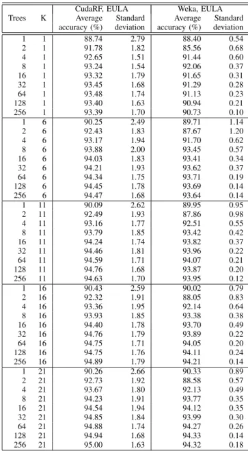
Table I presents the mean accuracy and standard deviation of CudaRF and Weka for k = 1, . . . , 21 and trees = 1, . . . , 256. With respect to classification performance, the average differ-ence between CudaRF and Weka RF across the 45 configura-tions is 0.935 − 0.923 = 0.012, which by no means can be regarded as significant. We assume that the existing difference can be attributed in part to the different attribute split measures and the difference in cross-validation stratification procedures. From the results in Table I we can conclude that CudaRF has comparable, and in most cases even higher, accuracy scores than Weka. This is an important result, in order to confidently assume that the CudaRF implementation generates at least as accurate classifications as a state-of-the-art implementation does.
TABLE I
CLASSIFICATION ACCURACY FORCUDARFANDWEKA FOR THEEULA
DATA SET.
CudaRF, EULA Weka, EULA Trees K Average Standard Average Standard
accuracy (%) deviation accuracy (%) deviation
1 1 88.74 2.79 88.40 0.54 2 1 91.78 1.82 85.56 0.68 4 1 92.65 1.51 91.44 0.60 8 1 93.24 1.54 92.06 0.37 16 1 93.32 1.79 91.65 0.31 32 1 93.45 1.68 91.29 0.28 64 1 93.48 1.74 91.13 0.23 128 1 93.40 1.63 90.94 0.21 256 1 93.39 1.70 90.73 0.10 1 6 90.25 2.49 89.71 1.14 2 6 92.43 1.83 87.67 1.20 4 6 93.17 1.94 91.70 0.62 8 6 93.88 2.00 93.45 0.57 16 6 94.03 1.83 93.41 0.34 32 6 94.21 1.93 93.62 0.37 64 6 94.34 1.75 93.71 0.19 128 6 94.45 1.78 93.69 0.14 256 6 94.47 1.68 93.64 0.14 1 11 90.09 2.62 89.95 0.95 2 11 92.49 1.93 87.86 0.98 4 11 93.16 1.77 92.51 0.55 8 11 93.79 1.85 93.42 0.42 16 11 94.24 1.74 93.82 0.37 32 11 94.46 1.81 93.96 0.22 64 11 94.59 1.71 94.07 0.21 128 11 94.76 1.68 93.87 0.20 256 11 94.63 1.70 93.95 0.12 1 16 90.43 2.59 90.02 0.79 2 16 92.32 1.91 88.05 0.83 4 16 93.36 1.95 92.14 0.64 8 16 93.93 1.85 93.38 0.38 16 16 94.40 1.78 93.70 0.49 32 16 94.76 1.79 93.89 0.22 64 16 94.75 1.71 94.05 0.20 128 16 94.75 1.76 94.11 0.24 256 16 94.89 1.79 94.21 0.14 1 21 90.26 2.66 90.33 0.89 2 21 92.73 1.92 88.58 0.57 4 21 93.67 1.80 92.13 0.49 8 21 94.23 1.91 93.77 0.35 16 21 94.54 1.94 94.12 0.35 32 21 94.85 1.84 93.99 0.30 64 21 94.88 1.74 94.27 0.26 128 21 94.94 1.68 94.33 0.14 256 21 95.00 1.63 94.32 0.18
B. Execution Time Results
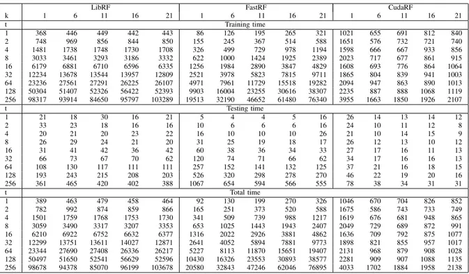
With regard to computation time, the experimental results clearly show that, for the studied classification task, CudaRF outperforms FastRF and LibRF. This is true in general, when the average result is calculated for each algorithm, but also for each specific configuration when the number of trees, k ≥ 10. The complete set of computation time results are presented in Table II. Local minima for LibRF and CudaRF can be found at k = 11 and k = 6, respectively, while the best k for FastRF is the lowest (1). We observe that when k is low and the number of trees is low, CudaRF has longer execution times than FastRF. This is mainly due to the fact the CudaRF has a higher initial overhead, for example, data transfer between the host and the device. However, as k is increased to levels
TABLE II
EXPERIMENTAL MEASUREMENTS OF TIME CONSUMPTION(MS)FORk = 1, . . . , 21AND TREES, t = 1, . . . , 256
LibRF FastRF CudaRF
k 1 6 11 16 21 1 6 11 16 21 1 6 11 16 21 t Training time 1 368 446 449 442 443 86 126 195 265 321 1021 655 691 812 840 2 748 969 856 844 850 155 245 367 514 588 1651 576 732 721 740 4 1481 1738 1748 1730 1708 326 499 729 978 1194 1598 666 667 933 856 8 3033 3461 3293 3186 3332 622 1000 1424 1925 2389 2023 717 677 861 915 16 6179 6881 6710 6596 6335 1256 1984 2890 3847 4829 1608 693 776 864 1064 32 12234 13678 13544 13957 12809 2521 3978 5823 7815 9711 1865 804 839 941 1003 64 23236 27561 27291 26225 26107 4971 7961 11729 15518 19282 2094 947 863 890 1013 128 50304 51407 52326 56422 52393 9903 16004 23255 30616 38307 2235 887 888 1068 1119 256 98317 93914 84650 95797 103289 19513 32190 46652 61480 76340 3955 1663 1850 1926 2107 t Testing time 1 21 18 30 16 21 5 4 4 5 16 26 14 13 14 12 2 33 23 18 16 16 10 6 6 6 16 24 10 11 12 8 4 20 21 20 23 22 16 10 10 10 26 21 10 14 15 9 8 26 29 24 21 20 31 25 19 18 17 26 12 13 10 12 16 31 41 42 36 42 60 38 36 34 33 27 17 16 11 13 32 66 73 67 70 62 120 74 71 66 62 34 17 16 16 13 64 108 130 117 111 111 257 152 141 132 125 37 21 16 18 15 128 193 243 215 208 203 526 320 298 278 270 46 22 19 20 16 256 361 465 420 402 388 1067 654 594 566 555 78 38 34 31 31 t Total time 1 389 463 479 458 464 92 130 199 270 326 1046 670 704 826 852 2 782 992 874 859 866 165 251 373 520 588 1675 586 743 733 749 4 1501 1759 1768 1753 1730 341 509 739 988 1217 1619 676 681 948 865 8 3059 3490 3317 3207 3353 653 1025 1443 1943 2407 2049 729 689 872 991 16 6210 6922 6752 6632 6377 1316 2022 2926 3881 4862 1636 709 792 875 1077 32 12299 13751 13611 14027 12871 2641 4052 5894 7881 9773 1898 821 855 957 1017 64 23344 27690 27408 26336 26217 5227 8113 11870 15651 19407 2131 968 879 908 1028 128 50497 51650 52541 56629 52596 10430 16326 23553 30893 38577 2281 909 907 1088 1135 256 98678 94378 85070 96199 103678 20580 32843 47246 62046 76895 4033 1702 1884 1958 2138
commonly used in applied domains (for example, k = 11 would be recommended by Weka for the EULA data set), CudaRF starts to outperform FastRF as the number of trees increases. For a low number of trees, the performance of LibRF is almost equivalent to the other algorithms but as the number of trees increases, the total time of LibRF increases linearly. In Figure 3, we present the speedup of CudaRF as compared to LibRF and FastRF, respectively, for the training phase, the testing phase, and totally. The results for the training phase show that the number of trees needs to be at least 8 (16) in order for CudaRF to be faster than LibRF (FastRF). Further, we note that the number of trees needs to be at least 32 in order for CudaRF to be faster than LibRF and FastRF in the testing phase. This is probably due to the fact that the test data contains relatively few instances. In practice, the number of instances in the test data set is usually much larger.
VII. CONCLUSIONS ANDFUTUREWORK
We have presented a new parallel version of the Random Forests machine learning algorithm, CudaRF, implemented using the compute unified device architecture. Our experi-mental comparison of CudaRF with state-of-the-art Random forests algorithms (LibRF and FastRF) shows that CudaRF outperforms both FastRF and LibRF in terms of computational time for the studied classification task (a data set featuring 996 instances defined by 1265 numeric inputs and a nominal target).
Unlike FastRF and LibRF, the proposed CudaRF algorithm executes on the graphics processing unit (GPU). In a regular consumer computer, the GPU offers a substantially higher
number of cores (processing units) than the CPU does. Since the difference in classification performance, i.e., accuracy, between the different Random Forests algorithms is negligible, it is evident that CudaRF is more efficient than FastRF and LibRF, especially when the number of attributes to sample at each split and the number of trees to generate grow. Our results show that CudaRF is approximately 30 times faster than FastRF and 50 times faster than LibRF for configurations where the number of trees is 128 and higher.
For future work, we intend to refine the CudaRF algorithm. In particular, we are going to add more features to make CudaRF even more relevant for use in real-world applications. For example, the current version of CudaRF can only process numeric input attributes and a nominal target attribute. More-over, it does not handle missing values.
REFERENCES
[1] L. Breiman, “Random forests,” Machine Learning, vol. 45, pp. 5–32, 2001.
[2] D. Geer, “Taking the graphics processor beyond graphics,” IEEE Com-puter, vol. 38, no. 9, pp. 14–16, Sep. 2005.
[3] “GPGPU: General-Purpose computation on Graphics Processing Units,” http://www.gpgpu.org.
[4] D. Steinkraus, I. Buck, and P. Y. Simard, “Using GPUs for machine learning algorithms,” in Proc. of the 8th Int’l Conf. on Document Analysis and Recognition, 2005, pp. 1115–1120.
[5] B. Catanzaro, N. Sundaram, and K. Keutzer, “Fast support vector machine training and classification on graphics processors,” in Proc. of the 25th Int’l Conf. on Machine Learning, 2008, pp. 104–111. [6] D. Tarditi, S. Puri, and J. Oglesby, “Accelerator: Using data parallelism
to program GPUs for general purpose uses,” in ASPLOS-XII: Proc of the 12th Int’l Conf. on Architectural Support for Programming Languages and Operating Systems, Oct. 2006, pp. 325–335.
[7] T. Sharp, “Implementing decision trees and forests on a gpu,” in Proc. of the 10th European Conf. on Computer Vision, 2008, pp. 595–608.
0 10 20 30 40 50 60 70 1 2 4 8 16 32 64 128 256
CudaRF vs. LibRF (training 3me)
k=1 k=6 k=11 k=16 k=21 0 2 4 6 8 10 12 14 1 2 4 8 16 32 64 128 256
CudaRF vs. LibRF (tes1ng 1me)
k=1 k=6 k=11 k=16 k=21 0 10 20 30 40 50 60 70 1 2 4 8 16 32 64 128 256
CudaRF vs. LibRF (total 2me)
k=1 k=6 k=11 k=16 k=21 0 5 10 15 20 25 30 35 40 1 2 4 8 16 32 64 128 256
CudaRF vs. FastRF (training 1me)
k=1 k=6 k=11 k=16 k=21 0 2 4 6 8 10 12 14 16 18 20 1 2 4 8 16 32 64 128 256
CudaRF vs. FastRF (tes.ng .me)
k=1 k=6 k=11 k=16 k=21 0 5 10 15 20 25 30 35 40 1 2 4 8 16 32 64 128 256
CudaRF vs. FastRF (total /me)
k=1 k=6 k=11 k=16 k=21
Fig. 3. The speedup of CudaRF as compared to LibRF and FastRF, respectively, for the training phase, testing phase, and totally. [8] B. Lee, “LibRF: A library for random forests,” 2007, http://mtv.ece.ucsb.
edu/benlee/librf.html.
[9] I. H. Witten and E. Frank, Weka: Practical Machine Learning Tools and Techniques. Morgan Kaufmann Publishers, 2005.
[10] NVIDIA Corporation, “NVIDIA CUDA C programming best prac-tices guide, version 2.3,” http://developer.download.nvidia.com/compute/ cuda/2_3/toolkit/docs/NVIDIA_CUDA_BestPracticesGuide_2.3.pdf. [11] G. Topic, T. Smuc, Z. Sojat, and K. Skala, “Reimplementation of the
random forest algorithm,” in Proc. of the Int’l Workshop on Parallel Numerics, 2005, pp. 119–125.
[12] M. Matsumoto and T. Nishimura, “Mersenne Twister: A 623-dimensionally equidistributed uniform pseudo-random number genera-tor,” ACM Transactions on Modeling and Computer Simulation, vol. 8, pp. 3–30, 1998.
[13] N. Lavesson, M. Boldt, P. Davidsson, and A. Jacobsson, “Learning to detect spyware using end user license agreements,” Knowledge and Information Systems, vol. 26, no. 2, pp. 285–307, 2011.
[14] R. Kohavi, “A study of cross-validation and bootstrap for accuracy estimation and model selection,” in Proc. of the 14th Int’l Joint Conf. on Artificial Intelligence, vol. 2. Morgan Kaufmann, USA, 1995, pp. 1137–1143.
[15] F. Provost, T. Fawcett, and R. Kohavi, “The case against accuracy estimation for comparing induction algorithms,” in In Proceedings of the Fifteenth International Conference on Machine Learning. Morgan Kaufmann, 1997, pp. 445–453.