Development and Evaluation of a Kinect based Bin-Picking System

(1)

1

Development and Evaluation of a Kinect based

Bin-Picking System

DVA 407

Masters Thesis in Intelligent Embedded Systems

School of Innovation, Design and Engineering

Mälardalen University, Västerås

By

Chintan Mishra Zeeshan Ahmed Khan

Supervisor

:

Giacomo Spampinato

Examiner:

Mikael Ekström

(2)

2

ACKNOWLEDGEMENT

First and foremost, we would like to thank and are whole heartedly grateful to our supervisor Giacomo Spampinato at MDH and Johan Ernlund at Robotdalen for their time, support, faith and patience. It was due to them that we were able to learn and grow not only academically but also as individuals in this project.

We would like to extend a special word of thanks to Fredrik and Batu for their valuable inputs and the experience on the subject. We are humbled by our friends and family for their support. A special thanks to Mikael Ekström for reviewing the work and suggesting important changes.Thesis work is tedious job and requires a lot of time. We are thankful to everyone who was in support and constantly motivating us towards success.

(3)

3

ABSTRACT

In this paper, an attempt has been made to explore the possibility of using Kinect sensor instead of the conventional laser depth sensing camera for object recognition in a bin-picking system. The hardware capabilities and limitations of the Kinect have been analyzed. Several state-of-the-art algorithms were studied, analyzed, tested under different conditions and their results were compared based on their accuracy and reproducibility. An insight has been provided on the future work and potential improvements.

Level: Advanced Level Master Thesis

Author (s): Chintan Mishra, Zeeshan Ahmed Khan

Supervisor: Giacomo Spampinato

Title: Development and Evaluation of Kinect Based Bin- Picking System

Purpose: The purpose of this thesis is to investigate, and evaluate the Point Cloud from Kinect camera and develop a Bin-Picking System using Kinect camera

Method: Evaluation has been done using comparative study of algorithms and testing them practically under different conditions

Value: This thesis aims to streamline the various algorithms that are currently being used in IT industry, specifically in computer vision. Aims to provide an extremely cheap alternative to bin picking

Keywords: Bin-Picking, Kinect , PCL, Spin-Image, SHOT, SIFT, RANSAC, Keypoints

ABBREVIATIONS

SHOT: Signature of Histograms for Local Surface Description

SIFT: Scale Invariant Feature Transformation

MRPT: Mobile Robot Programing Toolkit

CAD: Computer Aided Design

PCL: Point Cloud Library

(4)

4

1 INTRODUCTION

Bin-Picking is the process of picking up a specific object from a random pile of objects. These objects can be differentiated from each other based on their physical properties. Since the early days of industrialization, sorting objects and placing them in supply lines has been a major part of production. For instance, vibratory separators were used to separate solid objects from scrap. Inertial vibrations made the lighter objects fall farther away from the tray and the heavier objects much closer to the tray which separated the pile of heavier objects from the lighter ones. In some versions, apertures were strategically placed so that the smaller objects could be filtered through. These were simple in concept and design.

However, there was a major disadvantage. The equipment was noisy, prone to mechanical wear and tear and had comparatively high maintenance costs. Besides, they were not intelligent and required more man power, meaning greater cost to company. This system called for an alternative and that was where the idea of replacing it with a vision system was born. Vision systems would provide the platform on which the machines could be made intelligent and processes such as “Pick and Place”. It was less noisy and periodic maintenance costs could be reduced. Today, vision based Bin-Picking is used in many industries and especially in the automotive industry.

In its nascent days vision based systems were limited to 2D object recognition. These were simpler to implement but could manipulate the data only at a 2D level. Greater details of the object could not be captured. There were many adjustment requirements before capturing the environment for further image processing. The cameras were highly sensitive to subtle changes in the surroundings

The present day technology uses laser based cameras for object identification. It eliminates the high degree of sensitivity and adds a major feature, “depth data capture”. This means that an object and/or the surroundings will be reliable and closer to the actual object properties. The object or the

surroundings can now be “described” for different orientations in the 3D viewing platform. The aim of this work is to try and reach closer to the results of Bin-Picking (by laser) by using the Microsoft Kinect Camera. The single major motivation behind the use of Kinect sensor was the high design and installation costs of laser cameras. Kinect is available at an affordable price of USD 150 which is very cheap when compared to its big brother the laser. Another advantage is its portability and inbuilt hardware such as tilt motors that may have future implementation. On the other hand, Kinect has a lower accuracy and lesser immunity to lighting conditions.

The purpose of this thesis work is to explore the use of known vision algorithms on Kinect. In addition to providing results of these combinations, analysis of different combinations of algorithms will lead to determining their accuracy in identifying the object of interest. Identification is not only linked to software but also aspects such as optimal placement of Kinect and adjusting physical environment in order to minimize disturbances. Algorithms will be explained in detail so that the reader can

understand them in simple home environments and potentially continue working on them to take it to the next logical step of bin-picking and path –planning.

1.1 State of the art

Bin picking systems that make use of stereo systems have been widely researched. A study by Rahardja calculated the position and normal vector of randomly stacked parts with the use of a stereo camera which required unique landmark features, which are composed of seed and supporting features to identify the target object and to estimate the pose of the object [48][49].

(6)

3 A study by Wang, Kak, et al. used a 3D range finder directly to compute depth and shape of articulated objects. However, it was subject to occlusion due to low resolution of the range finder [49] [50]. Edge feature extraction techniques have been used for object recognition and pose estimation. It was

effective against objects with smooth edges [51]. There are some solutions available in the market such as “Reliabot 3D vision package”, “PalletPicker-3D” and “SCAPE Bin-picker” for simple cylindrical and rotational objects [46].

It is the aim in bin-picking applications to have a general solution to deal with objects of different sizes and shapes. In 2010, Buchholz, WinkelBach and Wahl introduced a variation of RANSAC algorithm called RANSAM. The objects are localized by matching CAD data with a laser scan and have been highlighted in their paper for good performance despite clutter [52].

Since the introduction of Kinect in 2010, it has been at the center of non-gaming applications. The focus of most of the researches till this date has been on human motion analysis [43] and recognition of hand gestures [44] [45].

2 PURPOSE

This thesis is going to investigate the possibility of using a Kinect camera as a “cost effective”

replacement to laser camera in bin-Picking. Many state-of-art algorithms are good candidates for laser cameras and have provided very accurate results in the recent past; however their implementation in Kinect is yet to be explored.

2.1 Thesis Structure

This thesis is divided into major sections covering the hardware analysis of the Kinect and the software aspect of the algorithms implemented. The hardware section describes the Kinect camera viewing limitations both with respect to itself and the environment, adjustments and its specification. Software part deals with exploring the appropriate algorithm on the basis of available data from Kinect. Different image processing algorithms and approaches will be combined and their results will be verified.

2.2 Scope of Thesis

This thesis includes evaluation and selection of algorithms for the possible replacement of laser camera by Kinect camera in bin-picking systems. An attempt has been made to study the performance of algorithms that generally have a good performance in laser cameras when used on a Kinect camera. The set up for using the Kinect camera with respect to factors such as viewing area, lighting conditions and optimal distance from the camera has been discussed. Data capture, feature computation, keypoint extraction, segmentation, clutter and occlusion analysis are in scope of this document. Gripping patterns as well as position estimation are out of the scope of this thesis.

This will contribute in the work towards exploring a low cost alternative to the existing laser camera solution. In addition, an analysis and understanding of the algorithms discussed can be applied to indoor small scale object matching using PCL so that its industrial applications can be explored in future.

(7)

4

3 HARDWARE AND SOFTWARE

3.1 Kinect Camera

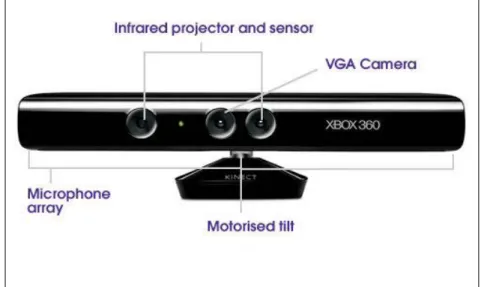
Kinect Camera is a motion sensor developed by Microsoft, based on RGB and depth camera. It works on depth sensing based on projection of IR (infrared) pattern on the environment and receiving the reflections from objects in the surroundings. It was developed as a Microsoft XBOX gaming console so that people can play games with the involvement of their full body rather than holding just a controller in hand. Kinect Sensor was launched in November 2010 and soon after its launch, programmers (Computer Vision) started hacking the sensor. Kinect is an extremely cheap product considering the availability of a depth sensor that changes the perspective of vision based recognition. Microsoft has released the Kinect SDK (Software Development Kit). Kinect camera now-a-days is in focus of development in motion sensing and object recognition fields. Some hardware details have been provided below.

Figure 1: Kinect Camera

 64 MB DDR2 SDRAM

 Two infrared cameras (CMOS & Color CMOS) and an IR projector.  Four microphones

 A Prime Sense PS1080-A2 Chip [19]  A 12-watt fan

 Pan and Tilt motor

A precaution here to observe is that the tilt head of the Kinect should not be tilted by hand. It may cause damage to the sensor [9].

(8)

5

3.2 Kinect Specification

The specifications of Kinect have been presented in many documents online [8] [9]

Property Value

Field of View 57◦ H, 43◦ V

Frame-rate 30 Hz

Spatial Range (VGA) 640 x 480 Spatial Resolution @ 2m

distance

3mm

Depth Range 0.8m - 4m

Depth Resolution @ 2m distance 1 cm

Table 1: Kinect Specifications

3.3 Point Cloud Library (PCL)

PCL is a stand-alone library [11], with numerous state-of-art algorithms for object recognition and tracking. The library is divided in several modules such as filters, features, geometry, keypoints etc. Each module is comprised of several algorithms. Pointcloud is a collection of points which refers to group of three dimensional points that is representing the properties of an object in x, y and z axis. There is an option also to represent the object in 3D.

PCL has been released under BSD License; so it is open source and everyone is eligible to participate in its development which is one of the reason that in regard of Robotics and Recognition programmers have put up such a collection of material in it that is useful for them and for others as well. The

repository is being updated every day and periodic releases are done.

3.4 OpenNI Driver

PCL (Point Cloud Library) has been used for the development and PCL provide OpenNI Driver for driving the Kinect Camera. OpenNI is an acronym of Open Natural Interface and a very profound name in open-source industry. There are many Application Programing Interface (API) and frameworks in the market from OpenNI [23] mainly for vision and audio sensors. Software programmers and software companies usually prefer API's from OpenNI because of robust rendering, reliability and stability. Programmers make modules of different functionalities in common use and organize collection of such modules usually known as a library. There are many libraries available such as OpenKinect, depthJS, SensorKinect, NITE etc. Two of them have been considered which are Point Cloud Library (PCL) and Libfreenect due to their application in wide number of projects and good open source support.

(9)

6

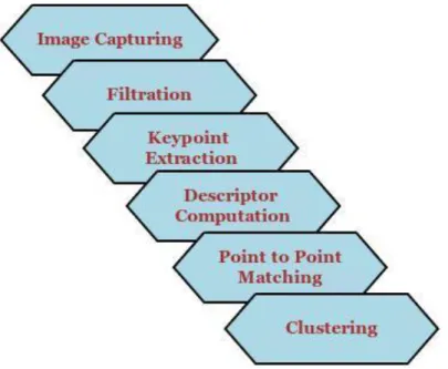
Figure 2: Image with Libfreenect driver

3.5 Software development model

Defining a solution verbally is considerably easy but while developing the solution one usually deals with number of problems. A good software development approach is to divide the problem in smaller chunks such that each chunk can be developed individually and later merged into a bigger solution. A “waterfall” model type approach has been adopted. This approach ensures that the development process is integrated in a sequential manner and provides a checkpoint after every functionality chunk to fall back on.

In this project, major functionalities have been considered as chunks. For instance, filtration has been considered as a major functionality which has been developed independently and later been integrated with the main program.

4 PRINCIPLE OF KINECT CAMERA

4.1 Depth Sensing

The principle behind depth sensing for the kinect is that an IR projector on the camera projects a speckled pattern of IR laser which is captured by an in-built infrared camera sensor. The image processor of Kinect uses the relative positions of the dots in the pattern to calculate the depth

displacement at each pixel position in the image [8] [10]. This principle is known as the principle of

structured light. The images captured by the camera are compared to a known pattern. Any deviation

from it can then determine whether the target is nearer or farther away. Figure 3 gives the actual picture of depth measurement in Kinect. Since the Kinect uses an IR sensor, it will not be working in sunlight

(10)

7 [10]. Besides, reflective and metallic surfaces are responsible for a lot of occlusion and ambiguous information.

Figure 3: Depth Camera [8]

In figure 3, it can be seen how depth estimate is calculated by the Kinect. The line of actual distance is the reflected IR beam. Based on this value, the depth value is calculated by Kinect. The nominal range accuracy of the laser scanner is 0.7 mm for a highly reflective target at a distance of 10 m to the scanner. The average point spacing of the point cloud on a surface perpendicular to the range direction (and also the optical axis of the infrared camera of Kinect) is 5 mm [31]. This means that for a good recognition, the object should not be placed too far from the camera sensor.

Figure 4: Depth Image

In figure 4, a depth image on the left and corresponding RGB feed to the right is shown. Varying distances are shown in different colors in the depth camera feed (left). It can be seen that the person in the image is closer to the Kinect and is shown in light green color. Similarly, the corresponding depth image background is shown in blue color. There were some ‘imperfections’ observed in the depth image. These imperfections are called clutter and occlusions. Clutter is the presence of noise where there is no real data and occlusion is the absence of data when the data is actually present. For instance,

(11)

8 the index finger, middle finger and ring finger of the left hand are seen cluttered whereas some portions behind the person appear dark due to occlusions. It is important to determine the optimum location of the Kinect for object detection in the bin-picking setup, so that clutter and occlusion is minimized.

4.2 Point Cloud

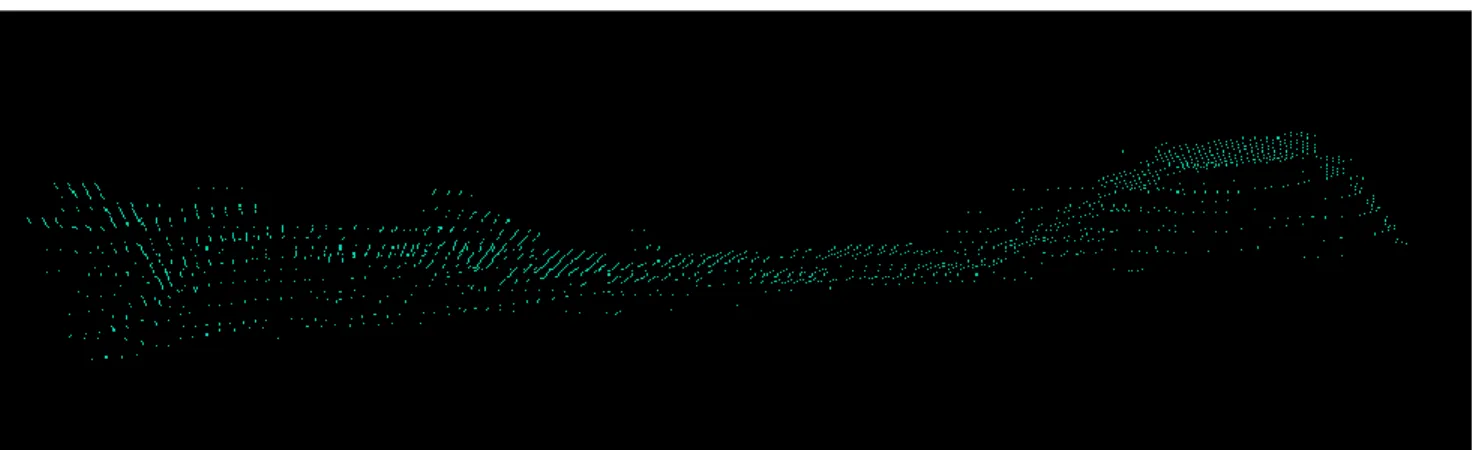
Kinect consists of a laser source that emits a single beam which is split into multiple beams by a diffraction grating to create a constant pattern of speckles projected onto the scene. This pattern is captured by the infrared camera and is correlated against a reference pattern [10]. The emitter is very powerful and the concept behind splitting it into multiple beams is to facilitate the use of a high power projector beam. This speckled pattern is interpreted by appropriate libraries (Point Cloud Library here) as a set of points known as ‘Point Cloud’. Each point on the cloud primarily has three co-ordinates X, Y and Z which are usually called vertices.

Point cloud can be explained with the analogy of a thin sheet of cloth. When objects are covered with this thin sheet, only an outline of their physical attributes such as shape and size can be seen. Sharp lines of distinction between covered objects and the background are not as good as without a sheet. If the figure 5, below is to be taken as an example, its clearly visible that IR Image of Kinect shows a ‘thin cloth sheet’ analogy. The only difference is that instead of a cloth there are group of points that define an object.

Figure 5: Point Cloud [21]

A usual pointcloud frame, from the Kinect has about 300000 points. Each point gives the orientation of the object/scene in space with respect to a specific viewpoint. It contains the orientation information as Cartesian co-ordinates. The default viewpoint of the camera is positive x-axis being the vector to the right, positive y-axis pointing downwards and positive z-axis being a vector pointing into the plane. Figure 3 shows how Kinect estimates the depth co-ordinate. Kinect works on scattering a stream of points in a range and then its IR camera captures the point cloud by Triangulation method.

A pointcloud can either be organized or unorganized. An organized pointcloud has an ‘image like’ organized structure. It comprises of a width and a height in the pointcloud which specify the number of

(12)

9 rows and the number of columns respectively [32]. In other words, it is arranged like a 2D array in the memory. It is easier to relate the points of an organized point cloud to its respective special co-ordinates. On the other hand, an unorganized pointcloud has all points stored as a 1D array.

5 RECOGNITION APPROACH

The open source libraries have predefined classes of many states of art algorithms with several parameters open for users to tame it as per their requirements. PCL has been preferred because of its advanced functionalities. It can handle complex geometric surface structures to be created thanks to a big number of points. The approach to object recognition can be summarized as follows:

Figure 6: Development approach

The methodology and motivation behind each stage have been highlighted in later sections. A

conceptual understanding at each stage has also been discussed so that the reader understands the basic concepts of these widely used algorithms that have been modified for recognition in 3D.

Image Capturing:

The image is captured and stored in a specific format. It has to contain data such as the 3D coordinates with respect to a defined reference axis, color information and/or gradient depending on the algorithm being used.

Filtration:

Filtration of the object under test is done to remove other unwanted objects in background to reduce clutter and occlusion in the captured image. It can be described as the process of “enhancing” an image by changing specific parameters. Unwanted information is neither time nor computation optimal. Besides, it also increases the chances of erroneous comparisons. The focus is to extract specific areas in

(13)

10 the object that would be unique to the object under test.

Keypoint Extraction:

Keypoints can be defined as distinctive features in an object or environment which can be used to perform object matching irrespective of its orientation in a scene. Keypoints reduce the number of points by “downsampling” the points. Simply put, downsampling can be defined as creating a new version of an image with a reduced size (width and height), which in turn takes lesser time to compute descriptors for all downsampled points.

Descriptor Computation:

A descriptor is computed that “describes” the object. For instance, say the given object is a pen which is 10mm in height. Say the pen is the only object among all other objects that has this unique 10mm height. If there existed a descriptor (some imaginary one) that calculates the distance between the top and the bottom vertex of an object, then this height would be how the object would be defined in the language of the descriptor. Hence, when this descriptor computes a value of 10mm, it would mean that the pen has been detected. The descriptors used in this thesis are 3D descriptors.

Point to Point matching:

After computation, the descriptors have been compared and good matches established based on a threshold value. These filtered good matches can then be clustered and classified to be belonging to a certain object instance. Explanation to matching can be found in section 5.5.

The whole process was applied to single isolated objects without clutter and occlusion like objects on a tabletop platform. This approach was then experimented on cluttered environments with similar

objects. Different combinations of these algorithms have been tried in order to get the optimal results. Keypoint extractions have been done using Uniform Sampling [1] and SIFT (Scale Invariant Feature Transform) [2]. To describe the object Spin-Image, SHOT [4] and PFH (Point Feature Histogram) [33] have been used.

It is important to understand the concept of normal estimation. Surface normals, as the name suggests are normal vectors perpendicular to a given surface at that point. A bigger surface is generally

subdivided into smaller surfaces. Plane tangents to these surfaces are drawn and the normals to these surfaces are computed. The angle between the normals of all these surfaces is a major contributor to determining the properties of the geometric structure and subsequent evaluation of descriptors.

Discussing it from PCL perspective, an important input provided by the user to calculate normals is the feature radius. The radius should be selected so that adjacent surfaces are not taken into consideration during normal estimation [34].

5.1 Image capturing

It is important to store the image for the model and the scene in a specific format. Images are stored in PCD (Point Cloud Data) format. PCD files consist of a header that identify and declare the properties of that format. A header contains entries such as version, fields, size, type, count, width, height, viewpoint, points and data. Image is captured in 3D containing information along X, Y and Z axes according to world co-ordinate system or camera co-ordinate system.

Additional information such as RGB information can also be captured. In this project, XYZRGB format has been used to capture the information of the scene. Users of PCL are given the choice of storing images in their own custom format. Count specifies the number of elements in each dimension. This feature is to allocate the ‘count’ number of contagious memory locations. A field called ‘Data’ specifies whether the type of data is ASCII or binary.

(14)

11 The obtained pointcloud can be stored as an organized or an unorganized pointcloud. An unorganized pointcloud means that all points on the pointcloud are stored in a 1D array i.e. the number of rows is one and the number of columns equal the total number of points in the input cloud. In an organized pointcloud the number of rows (height) and columns (width) are generally configured as 640 and 480 respectively. An advantage of organized pointcloud is that a mapping between depth pixel data and the corresponding RGB image structure (640 x 480) can be established after calibration of RGB and depth cameras. If Dm*n is a 2D depth image array and Cm*n is a 2D RGB image array, then an element Dij on

the depth image matrix would have the corresponding RGB information in Cij matrix that is the RGB

image matrix.

5.1.1 Creating a reference model

An object/s has to be defined in terms of different parameters such as color, orientation in space and their shape. These definitions of the given object are stored in the computer which is then used as a reference against other objects. The closer an object is to the properties of the stored object, the higher chance that both objects are the same. An object to be identified has to be compared against a reference model/s of object/s stored in the memory of the computer. The reference object can be matched to several objects in a scene or a single entity in the scene can be matched to a database of reference models. A reference model is supposed to be detailed and contain all the information regarding the object to be detected in a scene. The goal is to retrieve the smallest available information about the object in the scene and search for a match in the reference model or object database. Since the

reference model is detailed and contains information in all conceivable possibilities, there would be a higher probability of a good match and detection.

To create a model, a software tool called “Wings 3D” was selected. In the beginning, a simple cuboid model was constructed. The cuboid had to be converted into a pointcloud so that it could be stored and compared with a similar cuboid in the scene. This required the use of another useful tool called

(15)

12

Figure 7: Cuboid model in Meshlab

An option to add surfaces to the .obj file was selected to obtain a complete object. The model cuboid was then converted to its corresponding pointcloud format. A screenshot of the cuboid has been shown in figure 7. Total number of vertices and faces has also been provided by Meshlab. The object could be rotated in 3D and information about the frames per second and angle of view were also provided as default.

(16)

13

Figure 8: Pointcloud of cuboid model

The screenshot of the pointcloud model of a cuboid has been shown in figure 8. The pointcloud shown has only 8 points. It was seen that only the vertices of a given model were converted to the pointcloud and not the entire surface. It was difficult to obtain a good model with a few numbers of points. Hence, this approach did not give us the expected results.

The next approach was to obtain a CAD model from Solidworks and check if it could be converted to a pointcloud. A .stl file made in Solidworks was obtained for the test object. An object file to pcd

converter program (obj2pcd) was provided in PCL. Hence this .stl file was converted to an .obj using Meshlab which later was given as input to the PCL program. Pointcloud files have to be converted into ASCII format in order to be visualized in Meshlab.

(17)

14

Figure 9: Pointcloud of the CAD model

A pointcloud of the test object was taken as the reference model to be compared with a scene

pointcloud captured from the Kinect. The comparison techniques have been discussed in detail later in this report. The reference model did not show any match to the scene from Kinect. A little investigation led to the following conclusions:

I) After comparing coordinates of CAD model and Kinect scene model, it was found that the scale of the CAD model was different from Kinect scale.

II) The resolution of the pointcloud was much higher than the one obtained from Kinect. For comparison, it is desirable to have resolutions that are same or close.

The CAD model was scaled down in the X and Y coordinate by dividing each point by a factor of 1000. This scaled the model down to the Kinect scale of meters (The actual factor was 0.000966 but keypoints could be used to adjust these minor changes). The Z coordinate should not be changed; otherwise the shape of the model will be lost.

There are three parameters in the software tool to alter the resolution of the pointcloud: leaf size, resolution and level. Different combinations were tried but there was no appreciable match between the CAD model and the Kinect scene model.

In order to create a reference model, a pcd image of the object under test was captured with Kinect. Some reconstruction was applied to boost up the number of points and reduce the noise.

(18)

15

Figure 10: Pointcloud of the Kinect model before MLS

PCL library provides the implementation of an algorithm called Moving least squares (MLS) [29]. The output of the model after implementing MLS is shown in figure 11. MLS is a method for smoothing and interpolating scattered data [39], here it has been used to adjust the points in the cloud such that they can best fit the model. It is a modification of weighted least square (WLS) method. In order to understand WLS, least squares (LS) approximation technique has to be understood. The LS method minimizes the sum of squared residuals. A residual is similar to an error, only difference being that an error is difference between the observed value at a point and average value of all the points, whereas a residual is the error obtained by difference between the observed value and the average value of a “subset of random points” in the cloud. The optimum value will be when the total sum of the square of residuals is a minimum. In MLS, weighted least square is formulated for an arbitrary point for the points around it in a certain radius and the best fit is determined “locally” within the radius rather than globally as in WLS. The approximation is done by dividing the entire surface into smaller polynomials than solving for a large single system. The idea is to start with a weighted least squares formulation for an arbitrary fixed point in the pointcloud and then move this point over the entire parameter domain, in which a WLS fit is computed and evaluated for each point individually[40][41][42].

Figure 11: Pointcloud of the Kinect model after MLS

Though there was a marked improvement in the quality of the model, the model could not be matched with a different instance of the same object in a different orientation captured with Kinect.

(19)

16 words, the model was captured in different orientations from a fixed viewpoint and resulting pointcloud images were stored. These models were aligned to the first cloud's frame and the regions that were occluded in the first cloud's frame could be seen in other clouds.

Figure 12: Pointcloud of the model before ICP

The algorithm used for this purpose was Iterative Closest Point (ICP). The given reference model (captured from Kinect and filtered) and the sensed shape representing a major chunk of the data shape can be aligned by translating the scene cloud to the reference cloud. A fitness score is given based on the local minimum of the mean square distances between translations a relatively small set of rotations between the reference model cloud and scene cloud [30]. If the score was close to zero, it meant that the object cloud was a good fit to the reference and was included in the registration. This procedure was repeated for a single object in the scene placed in different orientations.

(20)

17 Comparing figures 12 and 13, it can be seen that the occlusion to the right has been compensated after ICP. In previous attempts, the model could not be compared to the scene at all. The ICP model served as a reasonable model because firstly, the model could be compared with the scene and secondly, it showed some good correspondences in a scene with similar objects. The descriptor parameters for comparison had to be trimmed for better results but this served as a good starting point.

5.1.2 Optimal placement of Kinect

It was visible earlier (figure 2) that the camera feed was not perfect. A limitation of Kinect with respect to distance from the Kinect has been illustrated. Some drawbacks with respect to the kind of objects that can be detected have also been shown. In figure 2, the left hand of the person in the picture is not clear and the fingers appear scarily webbed because of some noise which had corrupted the actual data. There are some regions in the picture that were observed to be blacked out. Some of these regions were either metallic or reflective. In some cases say in regions below the left arm, there was information but was not shown in the feed. This served as a strong motivation to check the depth information sensitivity of the Kinect. The images were subject to clutter and occlusions.

In simple terms, clutter can be defined as the presence of noisy data where there is no data present and an occlusion is when there is data actually present but is not detected by the camera sensor. The observations with clutter and occlusion set us on the path to minimize the clutter and occlusions. Hence, the first thing was to eliminate unwanted objects in the environment that would contribute to the noise. Putting the Kinect face down eliminated most of the objects in the surroundings; when the Kinect is facing the floor, only the floor and the objects placed on it were possible to be given as camera feed which minimized the noise. The viewing window of the Kinect would be uniform, hence leading to simpler segmentation and filtration algorithms.

The next step was determining the optimal distance to place the object for best possible detection. Setting the position of the Kinect was tricky because on one hand it should not be too near to the bin since it would hinder the movement of the pick and place robot and on the other hand, placing it too far away would clutter away the details of the object. It was observed that the information carried by the object reduces as a function if distance from the sensor. If the object is farther away, the neighboring IR projector particles would be farther away and could corrupt the actual information of the object with noise. Hence, closer the object, better the resolution. The object in consideration which had to be identified also had a hole of around 0.04 m in diameter.

The depth information sensitivity of the Kinect was analyzed from Openni (PCL) and libfreenect Kinect drivers. Libfreenect driver was the starting point to observe the depth sensitivity of the Kinect. There was significant color variations in the live depth image feed for depths > 1.5 cm in our

observations.

The first step in determining the sensitivity of Kinect sensor was to check the farthest possible distance it could detect an orifice. Generally, there is an increase in clutter with an increase in distance for an object sensed by the Kinect (away from the Kinect). The test object had detailed features and a hole. An orifice if detected will continue to lose information as it is moved farther away from the Kinect. There will be clutter and occlusions added to it.

(21)

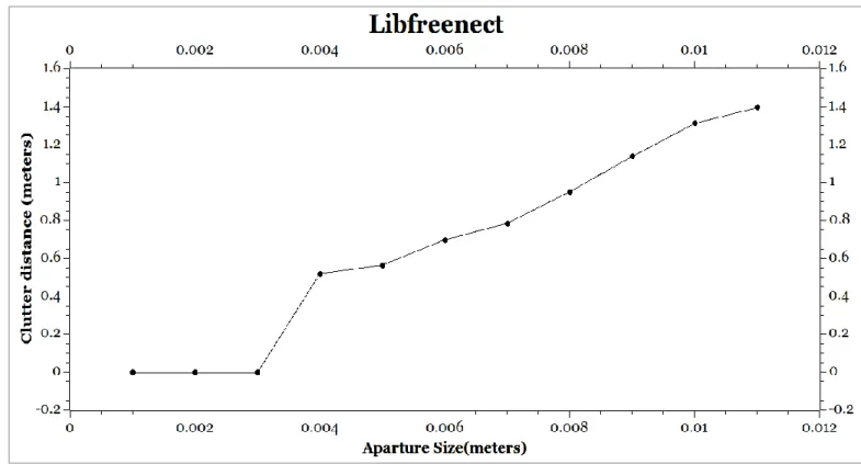
18 A monkey wrench was used for the purpose. Monkey wrenches have adjustable jaws. Measurements were made for a maximum aperture size (distance between the adjustable jaws) of 10-11mm. The measurements were started with 1mm as minimum aperture size The results shown below are the mean value of a number of measurements for a given aperture size. The following results were obtained for Libfreenect drivers:

Figure 14: Clutter graph for Libfreenect driver

The aperture size was kept at 1 mm and it was observed that the Kinect did not detect it and cluttered the 1mm gap with noise. Next the aperture size was increased to 2mm and still there was no detection and was shown cluttered in the camera feed. As the aperture size was increased, it was seen that at 4mm there was detection by Kinect at a distance of 60cm. However, if the aperture was kept at 4mm and moved further away, there was clutter observed again which confirmed that object details are corrupted with increase in distance from the Kinect. The maximum distance at which a certain aperture could be detected was plotted on the graphs. Similarly, other points too have been plotted in figures 14 and 9. For a given aperture size, ten such readings were taken and the mean value of the readings was used for the plot. The aperture size was increased by 1mm and a mean of ten measurements for that corresponding aperture size was repeated. The detection was appreciable after 4mm and not so good for lesser values.

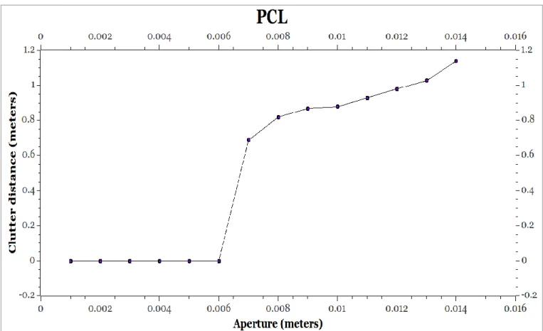
The experiment was repeated for Openni drivers. It was observed that the Kinect starts detecting the details well if the aperture size greater than 6mm. The detection was appreciable after 6mm and not so good for lesser values.

(22)

19 It was also seen that for higher values (not in figure 14) for Libfreenect drivers that the slope of the graph tends to dip. To be sure that it was not the driver responsible for the graphical pattern, the same test was carried out on Openni driver and the following results were observed:

Figure 15: Clutter graph for Openni driver

A software limitation of the Openni driver is obvious from the observations in the graphs above. It could be argued that Openni does not detect the aperture size as sensitively as Libfreenect since it starts detecting only if the aperture size is greater than 6mm and a distance of around 70cm and should not be considered. However, there is a major advantage that is mentioned later in this section.

The quality of the image decays as an object is moved farther away from the camera. It can be seen that the graph obtained from Openni and libfreenect drivers seem to “resemble” a logarithmic behavior. It could not be said for sure at this point but could be confirmed with the following tests.

In order to determine if there was any logarithmic relation between clutter distance and aperture, certain points in the graph were put in known mathematical equations to see if they behaved according to the equation. Two points were selected greater than aperture size of 8mm because that is where the graph starts resembling a logarithmic graph. It is known that slope of any logarithmic graph is less than 1 in the first quadrant of a 2D Cartesian co-ordinate system. Hence, the slope of the line between x-co-ordinates 0.85 - 0.9 cm was calculated.

(23)

20 I) The minimum slope on the graph was:

(y2- y1)

/

(x2-x1) = (0.88 – 0.87)

/

(0.01-0.009) = 10 θ = atan (10) = 84.29 degrees

The slope of the graph after 8 mm is not less than 45 degrees and hence cannot be a logarithmic graph. Besides, the slope was not decreasing for higher values of x as required logarithmic graph.

II) The second test was when a trial was done to fit the points in the graph to a logarithmic equation. The graph was shifted down in the negative Cartesian Y-axis by 0.69meters because this point is where the graph changed slope and hence is possible get a clear picture if the co-ordinate system is shifted such that these set of points could be fit into general logarithm function.

After the shift, the graph now cut the x-axis at x = 0.007. The modified logarithmic equation will be of the form:

y = logn(x+c); where n is unknown

A logarithmic graph cuts the x-axis at x=1. Hence, the value of c would be

c = 1-0.007 = 0.993

 y = logn(x+0.993);

Trial and error method was used and corresponding x, y (transformed y-coordinate) values in the graph were substituted. The results were checked for several values of n which was found to be 1.015 i.e.

almost 1. It is known that logarithms with base unity have indeterminate solution ruling out the

possibility of the graph obtained being a logarithmic graph based on our observations.

The above tests proved that the function could not be approximated with a logarithmic function. Nevertheless, our results and the graphs would be a major contributor in determining optimal position to place an object where the detection would show best results. For example, an object with aperture size of 10mm will have best detection approximately between 60-80mm (Figure 15) for Openni and between 60-110mm (Figure 14) for libfreenect respectively.

Libfreenect driver shows a linear behavior between 80-160 cm from the Kinect and smaller aperture sizes are detected better. On the downside, the construction of range-images from raw input point clouds can involve some loss of information as a result of multiple 3D points projecting to the same 2D range image pixel does not have a consistent graph for greater distances[26]. However, raw point clouds are a natural way to represent 3D sensor output point clouds are a natural way to represent 3D sensor output and there is no assumption of available connectivity information or underlying topology [26]. A pointcloud provides a better description of an object and this was the motivation to select Openni drivers for detection. These measurements highlighted the sensor limitations for a given model at a specific distance.

After trial and error it was decided that a distance between 1-1.2m would be good enough for experimental purpose.

5.2 Filtration

Pointclouds are detailed and contain a lot of information. Hence, it becomes increasingly more important to manipulate the image and exclude details that are not relevant. In the setup Kinect is facing the floor. This automatically reduces the chances of including objects in the scene that are not

(24)

21 important. Some objects are placed randomly so as to create a cluttered scene.

The starting point was to place a single test object and observe the scene. Noise could creep in despite the precautions and hence passthrough filter was included. A passthrough filter was implemented for the X axis and the Y axis setting the maximum limit on the viewing window of the Kinect. This

eliminated many surrounding points and reduced the noise and was implemented before applying plane segmentation.

There were some points corresponding to the object while the others belonged to the floor (in other words a “plane”). The first step was to isolate the points in the plane from the object which was done using RANSAC (Random Sample consensus) technique. This process is known as segmentation. Segmentation, as the name suggests is the process of dividing an image into regions that can be later split up for further analysis [27]. This technique was used to isolate the objects under test from the floor. In plane segmentation using RANSAC model, three random points are selected and a plane equation is generated. All other points in the scene are fitted to it and a check is done on whether they satisfy the equation. If they do, they are considered to be “inliers” in that equation.

This process is iterated for many points and the equation that has the maximum number of inliers is the “winner” and is the final confirmed plane equation [28]. All the points lying in the plane were isolated and subtracted away from the scene. The filtration technique was applied with increased number of objects and showed good results.

Segmentation with Kinect is highly sensitive to lighting conditions and the nature of the surface. It is advised here that the background object/s should not be highly reflective. After the procedures followed above if there was any noise then a SOR (Statistical outlier removal) filter was applied. SOR filter operates with the assumption that the distribution of points is Gaussian [11] [36]. It requires setting a threshold value for two parameters namely, the number of “K- neighbors” and standard deviation of the mean distance to the query point. A point on the cloud is selected and its proximity to the other points is calculated. If it lies within a certain proximity tolerance limit decided by the user, then the given point is said to be an “inlier” else it is said to be an “outlier”.

The proximity between two points can be calculated by Euclidean distance between them. Since the distribution of points has been assumed Gaussian, two parameters can be considered, namely the average or the mean distance between the points and the standard deviation. The distance threshold will be equal to:

Distance threshold = Mean + stddev_mult * stddev. [35][36]

Standard deviation multiplier has been set to 1 for simplicity. This value can be changed by trial and error based on the environment. Points will be classified as inlier or outlier if their average neighbor distance is below or above this threshold respectively. Filtration process can be summarized in the following flow:

Raw pointcloud data → Passthrough XY filter → Plane segmentation → SOR

5.3 Keypoint Extraction

Keypoints are specific regions or points that are unique to an object. These specific regions are invariant to the position and also to illumination to a certain degree which make them robust and reliable. These features have a high rate of good matches. The computation time of descriptors is also reduced because keypoints “downsample” the points thereby reducing the number of points meaning lesser descriptor computation time. Downsampling involves computing a weighted average of the

(25)

22 original pixels that overlap each new pixel [37].

The pointcloud data that has been obtained contain a lot of points and hence is heavy on the processor. These have to be downsampled to make them faster for processing. Though it is not a requirement in our project to achieve real-time solution, it helps save time. Points on a cloud which are close to each other usually have same characteristics. So, instead of selecting all of these points a few points termed as keypoints are extracted from them in a user defined region. In our case, the user defined region is the one obtained after segmentation and removal of outliers. There was another advantage of extracting keypoints. Tools are available that can be used for converting CAD models to pointcloud format. However, the pointcloud obtained from the object was very dense and had a different resolution from that of the Kinect setting resolution. The algorithms could not compare the object model and scene and downsampling of the model was necessary so that they could be compared with the actual scene. The reference model and the scene, both have to be of the same resolution for best results while

downsampling/extracting keypoints. This was because; earlier while creating a reference model section (section 5.1.1), downsampling resulted in data loss of details in an already sparse pointcloud

The effects of keypoint radius on recognition are presented in results section. Resolution of the pointcloud was 0.002m and hence radius of the keypoint was kept between 0.002m and 0.003m. This constraint on the keypoint would mean that all the surrounding points within this radius can be downsampled.

5.3.1 Uniform Sampling

In uniform sampling, a set of points that lie within an imaginary 3D cube of certain volume or voxel can be approximated with a single point representing the centroid of this cube or voxel. Uniform sampling not only down samples the pointcloud but also provides some filtration. Since downsampling involves the weighted average of new pixels, it reduces the number of invalid points. Uniform

sampling frames the pointcloud in 3D Grid as shown in figure 16.

The size of each voxel is user defined based on the level of downsampling aimed to achieve and the amount of detail desired to retain in the object [1]. For simpler objects, larger size for each voxel can be selected whereas for smaller objects and objects with a complex geometry, the voxel needs to be

smaller. An array of voxels in the cloud is known as voxel grid. Figure 16 shows single voxel and then the 3D grouping of voxels and voxel grid.

(26)

23

5.3.2 SIFT

SIFT is an acronym of Scale Invariant Feature Transformation. As the name suggests, these keypoints are invariant to change in scale and rotation. Kinect camera is very sensitive to minor changes in illumination which can affect the segmentation of the background from the actual scene before computing the keypoints. SIFT keypoints have partial invariance to change in illumination [2]. SIFT requires the point cloud to have either the RGB data or intensity data or both. The general idea of SIFT is explained below. SIFT computation can be divided into three stages:

a) A Scale space

In this step Gaussian blur function is applied incrementally to an image creating a “scale space”. The Gaussian smoothing operator is a 2-D convolution operator that is used to `blur' images and remove detail and noise [53]. Let us assume an image I(x, y, and z).

L(x, y, z, σ) = G(x, y, z, σ)*I(x, y, z)

The above is a convolution between Gaussian function and the image, where x, y, z are the coordinates, σ is a scaling parameter and L is the scale space [2]. The above equation has been explained for 2D [54] but the same logic is applicable for 3D in PCL. After the image has been progressively blurred, the resulting set of images is known as an octave. Hence, an octave contains a set of progressively blurred images of a given size. The size of the image can be changed multiplying or “scaling” it by a factor of 2. Several octaves can be constructed for each instance of a resized master image.

b) Laplacian of Gaussian

Differentiating the image to obtain edges and corners will be a time consuming process. Hence, the difference between two consecutive scales in an octave is

D(x, y, z, σ) = (G(x, y, z, kσ) - G(x, y, z, σ))* I(x, y, z) = L(x, y, z, kσ) - L(x, y, z, σ) [2]

In the above equation, D is the “difference of Gaussian”. The variable ‘k’ here is the factor by which the amount of blur differs in successive images for a given octave. Difference of Gaussian calculation is done for all the octaves present in the scale space.

c) Keypoint extraction

This is the step where the modification has been done for 3D. The original algorithm for 2D computes maxima and minima after obtaining the difference in Gaussian. Figure 17 shows the difference of Gaussian images in a given octave scale. Consider the pixel marked ‘X’ in figure 17. It is compared with its neighbors in the current scale and immediate neighbor scales. Hence the number of neighbors will be nine in the top scale, nine in the bottom and six pixels surrounding the pixel. If the difference of Gaussian value is greater than the neighbors' values then it is classified as local maxima and if it has the least value among all neighbors, it is classified as local minima.

In PCL, the pixel is a 3D point in the pointcloud. The neighbors or neighboring pixels here are the points lying within a search radius (a user input). A pixel can be classified as a keypoint if:

I) The difference of Gaussian value is an extrema (maxima or minima) and if it is an extrema for its own scale.

II) The point is also an extrema for the immediate smaller and immediate larger scales in the scale space.

(27)

24

Figure 17: Computing maxima and minima in an octave [2]

5.4 Descriptors

It is not enough if only the keypoints in a pointcloud are extracted. The image has to be made rotation invariant so that matching can be done regardless of the orientation of the object. This can be achieved by calculating descriptors. Object Recognition revolves around the concepts of Surface Matching and Feature Extraction. An object model has to be “described” or depicted based on characteristics of the surface of the object so that it can be matched based on these characteristics with other objects.

There are many profound state-of-the-art descriptor options today, but two of them namely Spin-Image [3] and SHOT [4] have been focused upon. Spin-Images are currently being used in the industry due to their high reliability, accuracy and robustness. SHOT is a recent development and has been shown to have a better performance than spin images [4].

5.4.1 Spin Image

Surface matching is the process of determining the similarity between shapes of two compared objects. In bin-picking scenario, things are complicated because of the amount of clutter and occlusion involved which meant that the descriptor should measure local surface properties. Besides, the objects in a bin are randomly oriented. Local surface properties aid in breaking down the scene into smaller chunks that can be compared with the features of the model for matching [6].

Spin-Image is an algorithm that provides the position of a point in 3D as a 2D co-ordinate

representation. They are rotation, scale and pose invariant [3]. The object surfaces are assumed to be regular polygonal surface meshes of a certain resolution. This is known as the mesh resolution. In other words mesh resolution can be defined as the median of all edge lengths in a mesh. Edge length means the distance between two adjacent points in a cloud. The mesh here would be the surface that would be obtained if all points in the pointcloud would be triangulated. The resolution of the Kinect pointcloud has been calculated in the program. A prerequisite to calculation of spin-image is to calculate the normals in the object model and in the scene. A normal to an oriented surface point in the cloud is a vector pointing perpendicular to the plane. Figure 18 gives an idea about the normal to an image.

(28)

25

Figure 18: Accumulation of bins in a Spin-Image

Each spin-image pixel is a bin that stores the number of surface points with the given radius (α) and depth (β) [7] [3]. Consider the plane in figure 19 that is rotating about the normal of a point. When it rotates, it sweeps neighboring points in the model. One such point has been illustrated in figure 18 where a neighboring point has been labeled “surface”. The radius and the depth give the local position of point on surface with respect to the test point at which normal has been drawn.

There are three parameters that govern the calculation of spin images namely image width, bin size and support angle. The surface points (α, β) (figure 18) are smoothened out by bilinear interpolation. These points have to be collected in a 2D matrix. This matrix can have any number of rows and columns but are collected in square matrices for simplicity. Image width decides the number of rows and columns in this square matrix [38]. The image width has been set to 8 in our implementation.

Figure 19: Sweep angle in a Spin-Image [3]

Bin size determines the maximum number of neighboring points that can be grouped together for a given point. The representations of all these points are in 2D. In PCL, bin size is calculated as follows:

Bin size = Search radius / Image Width

The search radius is a user input that considers all the neighbors in a specific periphery around a vertex. Bin size should be set equal to the spin-image resolution value for best results. A larger bin size means that more number of vertices will be included and larger the bin size, the lesser sensitivity to minute details [7].

The support angle is stored as the cosine of the angle of orientation. Spin-Image generation at an orientation point can be considered to be a plane sweeping a cylinder with its axis of rotation at the normal of the orientation point. The angle by which the plane rotates is known as support angle. In the picture above (Figure 19), as the plane swept the duck, it collected the neighboring points.

(29)

26 The sweep is determined by the third parameter which is the support angle (cosine of support angle). The support angle is selected to minimize clutter. If the value is 1 (cos 360) then it makes one complete rotation. The support angle has to be selected carefully. In a cluttered scene, more often than not, a complete rotation sweeps points that may belong to another object and wrongly be calculated as a feature of the same object. A sweep angle between 45 degrees and 90 degrees can impart the selective localization of the object and reduce the chances of including a feature of the other object.

The spin image descriptor calculated was stored in the form of a histogram. Bilinear interpolation gives a sort of “weighted average” from surrounding points that are collected by the rotating plane. It is these weights that are stored in the histogram. The histogram is a vector of 153 fields (17x9), but they can be adjusted to collect 64 fields (8x8) because image width has been set as 8.

After calculation of the spin images, they were compared by Euclidean distance measurement between the scene and the model. A perfect match would mean that the Euclidean distance is zero; hence, theoretically smaller the distance, better the match.

5.4.2 SHOT

SHOT is an acronym of Signature of Histogram of Orientation and was developed by Federico Tombari, Samuele Salti, and Luigi Di Stefano. This algorithm incorporates the best features of both signature and histogram way of describing a particular object [4]. It is a recent advancement in the field of image recognition and has proved to be a very accurate and powerful tool. SHOT is efficient,

descriptive and robust to noise [4].

In SHOT, an invariant reference axis is defined against which the descriptor is calculated describing the local structure around a point of the cloud under consideration. Descriptor of local structure around a given point is calculated based on a radius value input by the user for only the points within the support of the radius. The descriptor here is a histogram of 352 fields (descriptor length) which should be interpreted as a 2D 32x11 matrix. The maximum width of this histogram here is 11 (10+1) where 10 is the user input value. This input value "n” can be changed by the user to any value less than 10 if desired and would be taken up by PCL as (n+1).

Reference axis is based upon a spherical co-ordinate system [4]. Points around a feature point are collected within the defined radius input by user according to a “function of angle θ” and not θ alone, where θ is the angle between normal at each point within the support radius and the normal at the feature point [4]. The support angle range for a normal is [-π, π]; hence, if the user input is 10 and if the grouping were done based on θ alone, then each interval or “bin” of the histogram is as follows:

Bin 1 = [-π,-9 π/10), Bin 2 = [-9 π/10,-8 π/10), Bin 3 = [-8 π/10,-7 π/10) …

Say, if the inclination is between the normal at a feature point and another point is -19π /20, it should lay in the bin 2. But since the binning is done based on cos θ and not θ, the binning is done on a range of [cos (-π), cos (π)] i.e. [-1, 1]. Hence, the binning is also done accordingly.

Earlier in this section, it was observed that the binning was taken up as n+1 by PCL. Since the upper limit of the bin interval is always excluded, there might be an extra bin added to include the last value of the last bin.

(30)

27

Figure 20: SHOT structure [4]

5.5 Point Matching and Clustering

After the descriptors have been calculated, the model and scene have to be matched. The descriptors are matched based on Euclidean distances. The smaller the distance between the descriptor points, the better the match. In ideal conditions, the distance is supposed to be zero. In this project, the threshold has been kept at little above zero because it is impossible to have a perfect zero score.

After point matching stage, the points have to be grouped together so that they can be identified to belong to a particular instance of an object. Say, a point on the model matches with two points on the scene, the user should be able to determine that both points on the scene show the same feature but belong to different objects. This can achieved with the help of clustering which is out of scope in our project.

Clustering has not been explored deeply in this project and can be placed under future work. To begin with, Euclidean clustering can be looked into for identification of simple objects in the bin. This can be modified for complicated objects if desired by users.

6 RESULTS

The results have been presented based on the different scenarios. Several combinations of algorithms were tried for the best possible matches who have been presented in the subsections below. For each combination, threshold parameters were changed and the results were observed. However, it should be noted that threshold also depended on other parameters such as descriptor radius, keypoint radius, bin-size (for spin images) have been adjusted for best possible results for the test environment conditions in our set up. The same also applies to filtration and segmentation parameters that have been adjusted for the best conditions and discussed in the preceding sections.

The results discussed in this section have been analyzed on reference models and scene both of which have undergone filtration and segmentation. Results have been shown for scene conditions involving one object and for a scene involving many objects. Effect of descriptor radius and keypoint radius on segmented scenes has also been analyzed to aid future work and exploit the algorithms better.

PFH (Point feature Histogram) was the first algorithm under test. Correspondences between the reference object and the object in scene could not be established at regions where the pointcloud was sparse. PFH attempts to capture as best as possible the sampled surface variations by taking into

(31)

28 account all the interactions between the directions of the estimated normals [33]. A sparse pointcould will not provide enough neighbors for a point to compute the normals correctly. This will not be a correct representation of the surface, which in turn would affect PFH parameters. In this algorithm, PFH algorithm took a very long time of almost over 30 minutes to calculate correspondences without keypoints; the resultant correspondences were not good. However, in regions of the object with a dense pointcloud, a few good correspondences could be seen.

It is to be noted that PFH results were observed when the scene was filtered and without the presence of other objects. The long time it took despite these modifications along with which it also gave a lot of wrong correspondences made us search for better algorithms.

6.1 Spin Image

Spin Images were the automatic starting point for comparing images. It could be recalled that in earlier sections while making a model, they were given as input to the spin image algorithm. They were the first choice since they have been industrially implemented successfully. The results of spin comparison were not satisfactory though many good correspondences were obtained. Due to the limitations in the complexity of the object, there were a lot of wrong correspondences observed. Spin-Image gave good results on simple objects such as cubes and cylinders.

Two test environments were used. In the first was with only one object in the scene which was matched with the model stored in the computer. In the second scenario, there were many test objects placed in the scene in order to make it partially cluttered. By partially cluttered, it is meant that some of the objects were placed distinctly on the floor while a few others were placed one on top of another in a random manner.

To begin with, a scene with one object was selected and Spin image algorithm was applied to it. Here, changed threshold values were changed and the results were compared. Threshold value refers to the squared distance between two descriptors being cmpared. If the value between reference descriptor and scene descriptor is less than threshold value then the point is said to be a valid match.

Threshold values are decided by trial and error. In this experiment, a stringent threshold value of 0.1 was selected and results calculated. Next, the threshold was relaxed to a value of 0.25 and the results were noted down. These results were then compared against each other.

(32)

29

Figure 21: Correspondences with SPIN with threshold limit 0.25

LEGEND: ms - Milliseconds NA – Not Applicable

Threshold limit = 0.1

Keypoints Calculation time NA Descriptor Calculation time 126 ms Total Recognition Time 5719 ms Correspondences 1899

Results Partially good

Table 2: Statistics for single object matching for threshold=0.1

Keypoints Calculation time NA Descriptor Calculation time 127 ms Total Recognition Time 5874 ms Correspondences 1899

Results Partially good

(33)

30 The recognition time was very low but there were several wrong correspondences and can be seen from figure 21 above. Table 2 and table 3 do not have a major difference and changing the threshold value did not have a major impact on the results.

Keypoints Calculation time NA Descriptor Calculation time NA Total Recognition Time NA Correspondences NA

Results Error

Table 4: Statistics for cluttered scene for threshold=0.25

Table 4 shows the results for a cluttered scene for a threshold value of 0.25.

6.2 SHOT

The results here were better than the results obtained only with spin images. The number of wrong correspondences reduced and in the scenario with only one object in the scene, the number of

correspondences was very good. However, some wrong correspondences managed to creep in which were sorted out by lowering the threshold value in the scene. Similar to the tests in spin image, the threshold values of SHOT were changed and the results observed. To highlight the effect of threshold values, a threshold limit of 0.1 showcases stringent conditions. An increase in the value means that threshold has been relaxed.

Threshold values that are too stringent may lead to no matching at all as was seen with threshold value 0.1.After trial and error experiments it was found that 0.25 was the optimal value for threshold since higher values resulted in noise and incorrect correspondences. It should be kept in mind that it is descriptors in our project that are responsible for matching and keypoints are just for downsampling and scale invariance.

Keypoints Calculation time NA Descriptor Calculation time 10381 ms Total Recognition Time NA Correspondences 0

Results No match

(34)

31

Keypoints Calculation time NA Descriptor Calculation time 10439 ms Total Recognition Time 11437 ms Correspondences 77

Results Mostly good

Table 6: Statistics for single object matching for threshold=0.25

Figure 22: Correspondences with SHOT with threshold limit 0.25

A threshold of 0.1 gave no correspondences but a threshold value of 0.25 gave 77 correspondences. Most of them were very good. As seen in screenshot above (figure 22), it can be seen that the number of good correspondences are appreciably more than the bad correspondences. Though the recognition time was roughly twice that of spin images in section 6.1, they were more reliable

(35)

32

Figure 23: Correspondences with SHOT with threshold limit 0.25 for cluttered scene

Keypoints Calculation time NA Descriptor Calculation time 39791 ms Total Recognition Time 41691 ms Correspondences Not Calculated

Results Ok

Table 7: Statistics for single object match for threshold limit 0.25

The correspondences were better with SHOT compared to using spin image algorithm for cluttered scene in section 6.1. The better performance with single object environment was an early indication that SHOT may be a better option with Kinect than spin images. However, SHOT alone was not enough to give close to satisfactory results in a cluttered environment as evident from figure 23.

(36)

33

6.3 Uniform Sampling and SHOT

Uniform sampling was the first type of keypoint that was tried in our algorithms. In this section uniform sampling with SHOT has been used. Uniform sampling and SHOT showed good results for simple objects (cubes and cylinders). Our test object also showed good results for a single and isolated object environment. Isolated objects here mean objects in the environment were not overlapping each other. Some promising matches in a test cluttered scene were also observed.

Keypoints Calculation time 7ms Descriptor Calculation time 9124 ms Total Recognition Time 10028 ms Results No match

Table 8: Statistics for single object matching for threshold limit 0.1

Keypoints Calculation time 26ms Descriptor Calculation time 9193 ms Total Recognition Time 10433 ms Correspondences 77

Results Mostly good

Table 9: Statistics for single object matching for threshold limit 0.25

In table 9 it can be seen that there was no marked difference for single object identification with keypoints. The same number of correspondences was found when only SHOT was used. However it can be seen that the recognition time was reduced which highlights the use of keypoints.