Above- and belowground carbon stocks and effects of enrichment planting in a tropical secondary lowland dipterocarp rainforest

Swedish University of Agricultural Sciences, Department of Forest Ecology and Management Independent project in forest science • 60 credits

Master of Science in Forestry

Examensarbeten /SLU, Institutionen för skogens ekologi och skötsel • ISSN 1654-1898 Umeå 2019

Above- and belowground carbon stocks and

effects of enrichment planting in a tropical

secondary lowland dipterocarp rainforest

Joel Jensen

Examensarbeten

2019:9

Fakulteten för skogsvetenskap

Above- and belowground carbon stocks and effects

of enrichment planting in a tropical secondary

lowland dipterocarp rainforest

Joel Jensen

Supervisor: Ulrik Ilstedt, Swedish University of Agricultural Sciences, Department of Forest Ecology and Management

Assistant supervisor: Niles Hasselquist, Swedish University of Agricultural Sciences,

Department of Forest Ecology and Management

Examiner: Gert Nyberg, Swedish University of Agricultural Sciences, Department of Forest Ecology and Management

Credits: 60 credits

Level: Advanced level A2E

Course title: Independent project in forest science at the Department of Forest Ecology and Management

Course code: EX0913

Course coordinating Department of Forest Ecology and Management department:

Programme /education: Master of Science in Forestry Place of publication: Umeå

Year of publication: 2019

Cover picture: Joel Jensen

Title of series: Examensarbeten / SLU, Institutionen för skogens ekologi och skötsel

Part number: 2019:9

ISSN: 1654-1898

Online publication: https://stud.epsilon.slu.se

Keywords: Restoration, tree diversity, biodiversity, soil edaphic factors, functional species groups, liberation, forest degradation

Swedish University of Agricultural Sciences

Faculty of Forestry

I denna rapport redovisas ett examensarbete utfört vid Institutionen för skogens ekologi och skötsel, Skogsvetenskapliga fakulteten, SLU. Arbetet har handletts och granskats av handledaren, och godkänts av examinator. För rapportens slutliga innehåll är dock författaren ensam ansvarig.

This report presents an MSc/BSc thesis at the Department of Forest Ecology and Management, Faculty of Forest Sciences, SLU. The work has been supervised and reviewed by the supervisor, and been approved by the examiner. However, the author is the sole responsible for the content.

The intact tropical rainforests are rapidly being degraded and subsequently converted to other land uses, with associated greenhouse gas emissions and loss of biodiversity. It is imperative that the effects of such conversions and large-scale restoration efforts on forest structure and ecosystem services are understood to effectively be able to counteract the negative consequences of deforestation and forest degradation. Assisted regeneration by line planting is one such restoration method that have been used in degraded forests. Here I studied a chronosequence of 0-19 years since planting in a secondary lowland dipterocarp forest in Sabah, Malaysian Borneo which was selectively logged in the 1970s and subsequently burned at varying intensity in the El Niño fires 1983-1984 resulting in forests that are in arrested in early stages of succession. The primary focus of this study was the assessment of above- and belowground carbon in total, in different carbon pools and by functional species group (dipterocarps, fruit trees, pioneers and other commercial) in a secondary rainforest, as well as assessing the potential influence of assisted regeneration through enrichment line planting on these carbon pools as well as on tree diversity. I found no significant relationship in total carbon, carbon in different pools or carbon in different functional species groups and time since planting. Also, there was no significant difference in tree diversity or species diversity between treated and untreated control plots. Combining all 12 (60 x 60 m) plots, the mean total carbon stock (± SE) was estimated to 231.4

± 11.2 Mg C ha-1_{. This includes aboveground carbon pools: tree aboveground carbon (TAGC:}

44.0%, 101.7 ± 8.5 Mg C ha-1_{), woody debris (3.4%, 7.9 ± 1.5 Mg C ha}-1_{), standing dead wood}

(2.0%, 4.5 ± 1.0 Mg C ha-1_{), fine ground litter (FGL: 0.8%, 2.0 ± 0.1 Mg C ha}-1_{), lianas (0.6%,}

1.4 ± 0.4 Mg C ha-1_{) and belowground: soil organic carbon (SOC: 36.2%, 83.8 ± 8.2 Mg C ha}

-1_{), tree belowground carbon (TBGC: 9.3%, 21.6 ± 2.1 Mg C ha}-1_{), fine & coarse roots (3.6%, 8.4}

± 2.1 Mg C ha-1_{). When testing for correlations of effects over time since treatment by linear}

regression analyses, the applied treatment was not found to significantly improve carbon storage in total, by carbon pools or by functional species groups (p > 0.05), nor was it found to improve overall tree diversity or species richness (p > 0.05). However, between the treated and untreated

control plots, there was a 10% (~20 Mg C ha-1_{) increase in total carbon storage, which indicates}

that the treatment might still have a positive effect on carbon sequestration. Therefore, I performed a power analyses, which indicated that to significantly detect a such an effect (with a power of 0.8), I would have needed 5.5 times the number of plots. Additionally, soil edaphic factors (e.g. nutrients and texture) appeared to influence aboveground forest structure, both in terms of carbon storage and stem density, and may be contributing factors to why no clear positive effect of restoration was detected. For the twin goals of climate change mitigation and biodiversity retention, further study should be devoted to understanding the effects of restoration methods on secondary tropical rainforests and to what extent edaphic factors may influence aboveground forest structure.

Keywords: Restoration, tree diversity, biodiversity, soil edaphic factors, functional species groups, liberation, forest degradation

List of tables

2

List of figures

3

1

Introduction

5

2

Material and Method

8

2.1 Study site 8

2.2 Experimental design 10

2.3 Data collection 12

2.4 Calculations and data analyses 14

2.4.1 Carbon 14 2.4.2 Tree diversity 17 2.4.3 Statistical analysis 17

3

Results

19

4

Discussion

28

Acknowledgements

36

References

37

Appendices

44

Table of contents

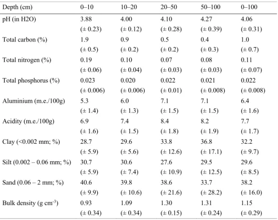
Table 1. Summary of soil edaphic properties from 12 plots within the INIKEA Sow-A-Seed project in Sabah, Malaysia, Borneo (± SD). 10

Table 2. Carbon content used for each respective organic carbon pool as a percentage of dry

mass. 15

Table 3. Model variables for Equation 2 (c: intercept, α & β: slope coefficients, CF: correction

factor). 16

Table 4. Carbon stocks and sequestration in tropical primary and secondary dipterocarp forests as well as in timber and oil palm plantations. 32

Appendix 1. Species identification (Malay vernacular name, binomial, genus and family), identified stems, functional species grouping and respective wood density for 12 (60 x

60 m) plots inventoried. 44

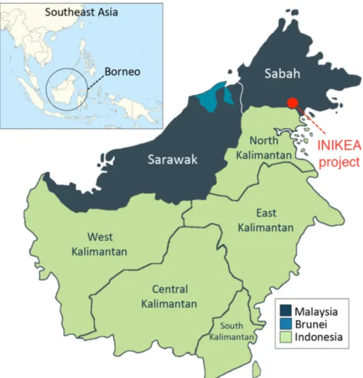
Figure 1. Location map of the INIKEA project area in the northern province of Sabah, Malaysian

Borneo. Published with kind permission from Daniel Lussetti. 9

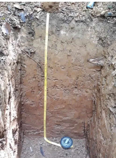
Figure 3. A photograph of a 1 m deep soil pit within the INIKEA project area is shown as an

example of the typical soil profile found in the plots this study. 13

Figure 4. Bar plot of above- (grey) and belowground (brown) carbon pools (Mg C ha-1_{) (± SE) of}

a secondary tropical forest in Sabah Borneo. Small dots represent the plot values from all 12 plots, regardless of time since restoration. 19

Figure 5. Box plot of total carbon in a degraded tropical forest (grey) as well as within areas of

assisted regeneration with enrichment line planting (brown). Enrichment line planting has occurred in three distinct planting phases (PP) which represents different ages since restoration. Y.S.P denotes approximate years since planting in the different planting phases whereas C represent untreated control plots. Small dots indicate plot values (n = 3 plots per planting phase and control). 20

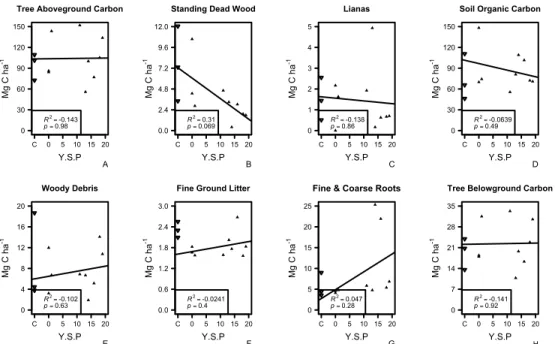
Figure 6. Linear regressions of carbon densities (Mg C ha-1_{) in the different carbon pools}

measured in this study over time since planting. Control plot values were not used in the regressions and are shown as hollow symbols as a reference. Y.S.P denotes approximate years since planting in the different planting phases whereas C represent

untreated control plots. 21

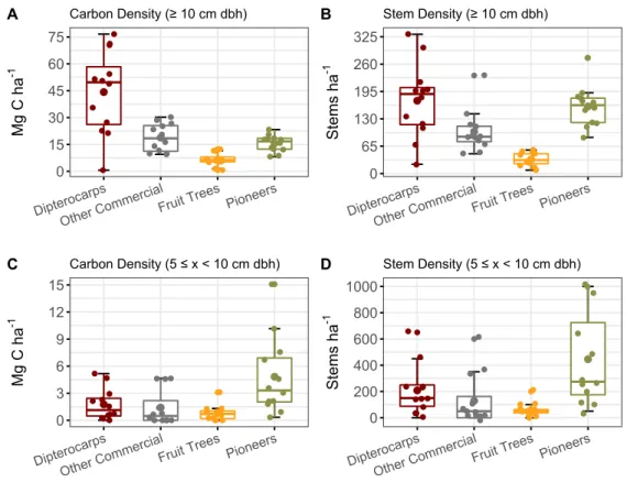
Figure 7. Box plots of carbon density (Mg C ha-1_{) and stem density (stems ha}-1_{) in large (≥ 10}

cm dbh; A, B) and small (10 > x ≥ 5 cm dbh; C, D) trees among the four functional species groups (dipterocarps, other commercial, fruit trees and pioneers) in a degraded tropical rainforest in Borneo. Small dots represent the plot values from all 12 plots, regardless of time since restoration. Error bars represent a 95% confidence

interval. 22

Figure 8. Linear regressions of carbon density (A) and stem density (B) for large (≥ 10 cm dbh) pioneers over time since planting. Data from control plots were excluded from the

regression analyses and are shown (hollow symbols) only for reference. 23

Figure 9. Linear regressions of Shannon´s diversity index (A and D), Pielou´s evenness index

(B and E) and rarefied species richness (C and F) over time since planting for large (≥ 10 cm dbh; A-C) and small (10 > x ≥ 5 cm dbh; D-F) trees. Control plot values were not used in the regressions and are shown as hollow symbols as a reference.

24

List of figures

Figure 10. Box plot of carbon density (A) and stem density (B) of large (≥ 10 cm dbh) and small

(10 > x ≥ 5 cm dbh) planted trees in the two oldest planting phases (PP). Y.S.P denotes approximate year since planting in the different planting phases.25

Figure 11. Linear regressions between soil clay (<0.002 mm; A), silt (0.002 – 0.06 mm; B) and

sand (0.06 - 2 mm; C) content and living and dead AGC. Living AGC (blue) represent carbon density in both trees and lianas, whereas dead AGC (yellow) represent the carbon density of woody debris, fine ground litter and standing dead wood.26

Figure 12. Linear regressions between soil phosphorus (A), nitrogen (B) and carbon (C) and

stem density in small (blue) and large trees (yellow) in all 12 plots. Soil texture particle sizes: clay (<0.002 mm), silt (0.06 - 0.002 mm) and sand (2 - 0.06 mm). 27

On a global scale, deforestation and forest degradation are occurring at a rapid pace which resulted in a net rate loss of 5.8 million ha of natural forest per year between 2010 and 2015 (Keenan, 2015). Such changes to natural forests have resulted in negative impacts on biodiversity, soil structure and water quality (WWF, 2019) as well as disturbing many vital ecosystems processes (Walker & Steffen, 1997). These changes also result in an increased emission of greenhouse gases to the atmosphere thereby enhancing global climate change (van der Werf et al., 2009). In particular, deforestation and forest degradation are extremely pervasive in tropical countries where the total area covered by primary forest has decreased by 62 million ha from 1990 to 2015 (Morales-Hidalgo et al., 2015). This is of extreme concern as many tropical forests are considered biodiversity hotspots (Botero et al., 2014) and host invaluable ecosystem services (Edwards et al., 2014). Thus, to combat the negative effects of deforestation and land degradation in the world’s tropical rainforests, there is a pressing need to identify effective approaches to conserve and restore these forested landscapes.

The forests of Borneo are known for their species abundance, harbouring approximately 15000 plant species, of which 3000 are trees (MacKinnon et al., 1996). The majority of forests on Borneo are classified as lowland rainforests (< 500 m a.s.l., > 2500 mm annual rainfall) and are regarded as biodiversity hotspots (Slik et al., 2003) that are dominated by trees in the Dipterocarpaceae family (Whitmore & Burnham, 1975). Forests in this area have experienced large-scale logging and severe droughts in 1982-1983 which led to natural wildfires in that burned ca. 1 million hectares of lowland tropical forest in the Malaysian province of Sabah (Malingreau 1985; Beaman et al. 1985). These disturbances have transformed the landscape into forests that are arrested in early stages of secondary succession.

Recently, there has been increasing interest in identifying different restoration practices that can be used to assist the recovery of ecosystem services in degraded tropical forests. One restoration practice that has received a lot of attention is assisted regeneration with enrichment planting. This approach involves the planting of selected native tree species into degraded forests while at the same time trying to minimize negative effects to- and promoting natural regeneration of valuable species that are already present (Montagnini

et al., 1997; Weaver, 1987). Assisted regeneration with enrichment planting can be

applied in various ways yet one of the most common approaches is through the use of enrichment line planting. In this approach, 2-meter-wide transects are cleared in degraded tropical forests and nursery-raised seedlings are then planted within the cleared transect (Ådjers et al., 1995; Appanah & Weinland, 1993). This approach has previously been applied in Vietnam (van Kuijk, 2008) and Brazil (Pena-Claros et al., 2002) and have in both cases been shown to successfully aid in the restoration of degraded tropical forests. In general, it is commonly assumed that enrichment line planting is an effective method of restoring degraded tropical forests (Bebber et al., 2002; Montagnini et al., 1997; Lamb, 1969), yet there is still a scarcity of long-term analysis regarding the effectiveness of assisted regeneration, line planting or other restoration methods (Reid et al., 2015; Hector et al., 2011). In addition to being labour-intensive and financially expensive, it takes many years, or even several decades, for significant effects to become apparent (Fisher et al., 2011; Chazdon et al., 2009). Thus, we still have limited knowledge about how assisted regeneration with enrichment planting may affect forest structure and ecosystem services, especially when considering multiple ecosystem services (Hector et al., 2011; Diaz et al., 2004). Consequently, there is a pressing need for more long-term studies to better assess the successfulness of this approach when restoring degraded tropical forests.

In 1998, the Swedish furniture company IKEA, in collaboration with the Swedish University of Agricultural Sciences (SLU) and the Malaysia forestry organization Yayasan Sabah created the Sow-A-Seed project, with the main objective of assisting the recovery of degraded tropical forests thereby improving the biodiversity and other ecosystem services (i.e., carbon sequestration) in an 18,500 hectare area in the Sungai Tiagau Forest Reserve in Sabah. Other projects in Sabah, Malaysian Borneo with similar goals to the Sow-A-Seed project include the INFAPRO project and the Sabah Biodiversity Experiment of the Malua Forest Reserve which covers 25,000 and 500 hectares respectively (Hector et al., 2011; Moura-Costa, 1996). The Bonn Challenge (IUCN, 2011), the New York Declaration on Forests (Summit, 2014) and the designation of 2021-2031 as the United Nations Decade on Ecosystem Restoration (UN, 2019) all indicate a growing global interest in large scale ecosystem restoration. To increase the chances of success for these and other projects it is crucial to understand

how different restoration approaches affect forest structure, including carbon stocks, as well as other ecosystem services.

In this study, I measured tree diversity and total carbon storage, including both above- and belowground pools within the Sow-A-Seed project with the main objective of trying to better understand the effects of enrichment line planting in a degraded lowland tropical rainforest. Moreover, given that enrichment line planting within the Sow-A-Seed project has occurred over a range of roughly 20 years we have the unique opportunity to assess the amount of time needed to observe significant effects of enrichment line planting in a degraded tropical rainforest. The data collected in this study provides a unique opportunity to assess the effects of the combined treatments of enrichment line planting and liberation applied to a degraded tropical rainforest by allowing us to consider the inclusion of belowground edaphic factors and their effect on aboveground forest structure which is rare for this type of study (Paoli et al., 2008). Additionally, the long-term nature of the study material, with subject areas as old as 19 years since planting (Y.S.P), further sets this study apart and will hopefully contribute new insights to the advancement of restoration ecology. Hence, my main objective of this study was to assess the effects of enrichment line planting and liberation on disturbed tropical rainforests regarding carbon sequestration and overall tree diversity. Specifically, I wanted to answer the following research questions:

• What are the total carbon stocks, including both above-and belowground carbon pools, of a secondary lowland dipterocarp tropical rainforest? • Do the restoration methods of assisted regeneration with line planting and

liberation (also known as enrichment line planting) affect above- and belowground carbon stocks?

• Does enrichment line planting increase the carbon and stem density of “desired” (dipterocarps, other commercial and fruit trees) functional species groups as well as overall tree diversity?

2.1 Study site

This study was conducted within the INIKEA Sow-A-Seed project, in the Sungai Tiagau Forest Reserve in the northernmost province of Sabah, Malaysian Borneo (4°38’44.7”N 117°16’24.8”E). The restoration project was initiated in 1998 with the main goal of improving biodiversity and at the same time assist the recovery of other ecosystem services (e.g. carbon sequestration) in an 18,500 degraded, secondary forest. Prior to logging in the 1970s and wildfires in the early 1980s, this area was characterized by trees in the Dipterocarpaceae family typical of lowland rainforests in the area (Whitmore & Burnham, 1975). After the fires in the early 1980s, pioneer trees, namely

Macaranga spp., became the dominating tree species and even to date these pioneer

trees are still dominant in these forests. Thus, much the forest within the INIKEA Sow-A-Seed project could be classified as being arrested in early stages of secondary succession. The geographical landscape is predominately made up of high hills and steep slopes, the climate is warm and humid, with a mean annual temperature of 27 and a mean (± SD) annual precipitation of 2517 ± 760 mm (based on measurements taken from 2002-2013; Gustafsson et al. (2016)).

Figure 1. Location map of the INIKEA project area in the northern province of Sabah, Malaysian Borneo.

Published with kind permission from Daniel Lussetti.

The soils of the study site are, by the SoilGrids system (Hengl et al., 2017), classified as Udults (USDA, 2014) and according to WRB are referred to as Haplic Acrisols (IUSS Working Group, 2006). These soils are typical of humid tropical climates and often highly acidic (Dahlgren et al., 2008). More detailed information about soil properties within the study area is presented below in Table 1.

Table 1. Summary of soil edaphic properties from 12 plots within the INIKEA Sow-A-Seed project in Sabah,

Malaysia, Borneo (± SD).

2.2 Experimental design

The field data were collected during two time periods, September-November 2017 and September-November 2018. Within the project area, 12 (60 x 60 m) plots were selected for measurements of tree diversity and total ecosystem carbon stocks. Nine plots were located in areas that were treated with enrichment line planting and liberation while three plots were located in untreated degraded, secondary forest and were used as control. The planting program was divided into 5-year long phases with planting phase 1 starting in 1998-2003, phase 2 ranging between 2003-2008, phase 3 between 2009-2013, and phase 4 from 2014 until current. Plots were selected based on being relatively easy to access from a nearby road yet being at least a 200 m distance from the road. Areas which would not be part of normal restoration operations (e.g. ravines, rivers, etc.) were avoided when deciding upon plot location.

Enrichment line planting is a method of restoration through assisted regeneration that is used to counteract the negative effects of forest degradation by attempting to recreate the natural forest and its dynamics in a target area (Montagnini et al., 1997; Weaver,

Depth (cm) 0–10 10–20 20–50 50–100 0–100 pH (in H2O) 3.88 (± 0.23) 4.00 (± 0.12) 4.10 (± 0.28) 4.27 (± 0.39) 4.06 (± 0.31) Total carbon (%) 1.9 (± 0.5) 0.9 (± 0.2) 0.5 (± 0.2) 0.4 (± 0.3) 1.0 (± 0.7) Total nitrogen (%) 0.19 (± 0.06) 0.10 (± 0.04) 0.07 (± 0.03) 0.08 (± 0.03) 0.11 (± 0.07) Total phosphorus (%) 0.023 (± 0.006) 0.020 (± 0.006) 0.022 (± 0.01) 0.021 (± 0.008) 0.022 (± 0.008) Aluminium (m.e./100g) 5.3 (± 1.4) 6.0 (± 1.3) 7.1 (± 1.5) 7.1 (± 1.5) 6.4 (± 1.6) Acidity (m.e./100g) 6.9 (± 1.6) 7.4 (± 1.5) 8.4 (± 1.8) 8.2 (± 1.9) 7.7 (± 1.7) Clay (<0.002 mm; %) 28.7 (± 5.9) 29.6 (± 5.6) 33.8 (± 12.6) 36.8 (± 17.1) 32.2 (± 9.7) Silt (0.002 – 0.06 mm; %) 30.7 (± 5.9) 30.6 (± 7.4) 27.6 (± 10.9) 29.5 (± 12.5) 29.6 (± 8.5) Sand (0.06 – 2 mm; %) 40.6 (± 9.9) 39.8 (± 10.6) 38.6 (± 21.6) 33.7 (± 28.2) 38.2 (± 16.0) Bulk density (g cm-3_{) 0.93} (± 0.34) 1.09 (± 0.34) 1.30 (± 0.15) 1.31 (± 0.24) 1.15 (± 0.29)

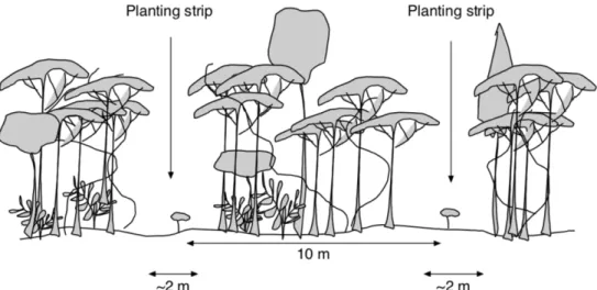
1987). The enrichment line planting is carried out in 2-meter-wide transects spaced at 10-meter intervals that are cleared of small trees without economic value, bushes and other ground vegetation (Figure 2.). If the terrain permits, seedlings are planted every 3 meters along the cut transects giving a maximum density of 330 seedlings per ha (Alloysius, 2010). The seedlings used for planting varies depending on what was available at the time of planting although the standing rule for species composition for field planting is approximately 70% dipterocarps, 25% other commercial and 5% fruit

trees with at least 25 different species per 200-300 ha planting block (Alloysius, 2010).

The liberation consists of the selective girdling of pioneer trees, primarily Macaranga spp., in and between the planting transects and the cutting of lianas throughout the area (Garcia et al., 2002). Maintenance lasts up to 10 years after planting and includes shade-adjustment up to four times and weed-slashing once per year. The shade-shade-adjustment consists of removing pioneer tree species and small trees to open up the canopy for the seedlings, while the weed-slashing consists of removing weeds and bushes. Resupply of seedlings was performed if the seedling survival rate was below 65% after 3 years since initial planting (Alloysius, 2010).

Figure 2. Enrichment line planting. Illustration of the enrichment line planting restoration method used in the INIKEA Sow-A-Seed project. Seedlings are planted every 3 meters in

2-meter-wide transects spaced at 10-meter intervals (Garcia et al., 2002).

The INIKEA project categorizes tree species into four functional species groups:

dipterocarps, other commercial, fruit trees and pioneers. Trees belonging to the species

group dipterocarps are species within the Dipterocarpaceae family. Pioneers are fast-growing trees that are not shade-dependent (ex. Macaranga spp. and Mallotus spp.) and are seen as undesirable as they add little value in terms of supporting biodiversity while

at the same time having low economic value and inhibiting the growth of other more valuable trees by outcompeting them. Fruit trees are trees that produce fruits annually that are valuable to local birds and animals, such as wild mango (Mangifera spp.) and durian trees (Durio spp.). Tree species belonging to other commercial are species that do not belong to dipterocarps or fruit trees but are still helpful to the restoration effort, examples include the Bornean ironwood (Eusideroxylon zwageri) and Merbau (Intsia

palembanica). The functional species group for individual species in this study are

presented in appendix 1.

2.3 Data collection

Dominant slope gradient and its bearing were determined with clinometer and compass respectively for each subplot in every plot. GPS coordinates were taken from the centre of every plot (Garmin inReach Explorer+).

The dbh (diameter breast height at 130 cm) of all trees, standing dead wood and lianas ≥ 10 cm dbh were measured, identified and tagged within each 60 x 60 m plot. Smaller trees, standing dead wood and lianas 10 > x ≥ 5 cm dbh were measured in a similar way in two 10 x 10 m subplots within each plot. Trees were identified to local vernacular, determined if they were within a 2 m planting transect and whether or not they were planted as part of the enrichment line planting by trained forest rangers. For trees with large buttresses, dbh was measured 0.3 m above the highest buttress. Additional measurements were taken for standing dead wood compared to live trees; height was visually estimated and decay class was determined (see woody debris).

Woody debris was collected from within 1 meter wide transects that were located along the outer edge of the 60 x 60 m plots (n = 2-4 transects per plot). All dead wood ≥ 2 cm on the ground within the transect were included in the data collection unless identified as having fallen from already dead trees or if the more than 50% of the dead wood was below the ground surface. Woody debris included in the data collection was categorized into decay classes depending on their decomposition, class 1 being fresh, newly dead wood and class 3 being highly decomposed (Chao et al., 2008). The collected woody debris was separated by corresponding decay class and weighed for fresh mass in the field for each plot. For large woody debris that could not be weighed, the length and diameter at each end was measured. Representative subsamples of each decay class for each plot were dried to constant weight to determine their respective dry mass fraction.

Fine ground litter (FGL) was collected within 8-9 subplots per 60 x 60 m plot from 0.5 x 0.5 m quadrants located in the centre their respective subplot. All dead organic matter was collected from inside the squares as long as it was readily identifiable as material derived from branches (< 2 cm), leaves, fruit, flowers or seeds. Dry mass fraction was determined by drying representative subsamples to constant weight.

Soil samples were collected in each plot from five depth intervals (organic, 0-10, 10-20, 20-50 and 50-100 cm). The samples from the organic, 0-10 and 10-20 cm depths were collected using a 5 cm deep metal cylinder, while a 10 cm deep metal cylinder was used for the samples from the 20-50 and 50-100 cm depths. One sample for the organic, 0-10 and 10-20 cm layers was collected from the centre of 8-10 randomly chosen subplots. In addition, a pit was dug to a depth of 1 m (Figure 3.) just outside each 60 x 60 m plot.

Figure 3. A photograph of a 1 m deep soil pit within the INIKEA project area is shown as an example of

the typical soil profile found in the plots this study.

From the deep pit, three samples were collected from the tree shallower depths (organic, 0-10, 10-20 cm depth), and samples were also collected centred at a depth of 25, 35 and 45 cm (for the 20-50 cm interval) and at 65, 75 and 95 cm (for the 50-100 cm interval). Samples from the depths of 0-10 and 10-20 cm had a volume of 203.47 cm3 _{while the}

samples from the depths of 20-50 and 50-100 cm had a volume of 406.94 cm3_{. For each}

soil sample, all roots and stones were removed, and the sample was homogenized and weighed for fresh mass. Roots from individual soil samples were sorted into two classes:

fine roots < 2mm and coarse roots > 2 mm) before they were dried to constant weight to determine dry mass and root density (g cm-3_{). Stones were weighed for mass and their}

volume was determined by the water displacement method. To determine dry mass fraction of soil samples, subsamples were weighed for fresh mass, dried in a 105 °C oven until constant weight was reached and then weighed for dry mass. Three samples per horizon per plot were used to determine their respective bulk density, the deeper samples correspond to the samples collected at 25, 35 and 45 cm for the 20-50 cm interval and at 65, 75 and 95 cm for the 50-100 cm interval (Equation 1.).

!" (% &'(_{) =}

+,_{-./01'234 8640ℎ '100: ∗ -1'234 8640ℎ '100<}-./01'234 567 '100

-1'234 =>3.'4 (1)

The soil samples were analysed at the laboratory of the Forest Research Centre, Sepilok, for pH (H2O), total phosphorus, total carbon, total nitrogen, exchangeable acidity, aluminium and texture. The plant samples were analysed for total carbon & nitrogen. Soil texture was determined following the particle size distribution test by Day (1965). Soil pH was measured in a 1:2.5 ratio of soil to pure (deionised) water using a glass-calomel electrode. Total carbon and total nitrogen were determined by dry combustion at 900°C using an Elementar Vario Max CN analyser (Elementar Analysensysteme, Hanau, Germany). Extraction for total phosphorus was carried out following the sulphuric acid-hydrogen peroxide digestion procedure described in Allen (1989) and the phosphorus contents in the digest determined using the molybdenum-blue method described in Anderson and Ingram (1993) at 880 nm on a spectrophotometer (HITACHI UV-VIS, Japan). To measure the exchangeable acidity, the soil was leached with 1M potassium chloride and titrated with 0.1N sodium hydroxide to a pink phenolphthalein endpoint (Anderson & Ingram, 1993; Thomas, 1982). For exchangeable Al in the leachate, a few drops of 0.01N HCl was added to the titrated solution to clear the pink colour, 1N KF was then added and the solution titrated with 0.05 M HCl to a colourless endpoint (Thomas, 1982).

2.4 Calculations and data analyses

2.4.1 Carbon

In this study, I refer to tree aboveground carbon (TAGC), standing dead wood, lianas, woody debris and fine ground litter (FGL) as aboveground carbon pools, and tree belowground carbon (TBGC), soil organic carbon (SOC) and fine & coarse roots as belowground carbon pools. To determine the total carbon stocks, each organic carbon

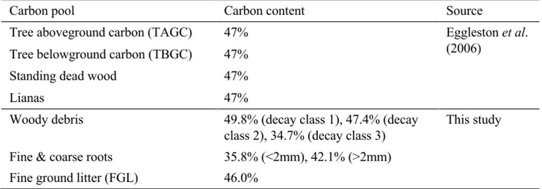
pool (all except SOC) was first estimated as dry biomass separately, and then multiplied by its corresponding carbon content to determine the amount of carbon in individual carbon pools. The carbon contents of this study varied by carbon pool and are shown in Table 2. The carbon contents of the SOC is not shown in Table 2., as it varied by both plot and soil depth.

Table 2. Carbon content used for each respective organic carbon pool as a percentage of dry mass.

Carbon pool Carbon content Source

Tree aboveground carbon (TAGC) 47% Eggleston et al. (2006) Tree belowground carbon (TBGC) 47%

Standing dead wood 47%

Lianas 47%

Woody debris 49.8% (decay class 1), 47.4% (decay class 2), 34.7% (decay class 3)

This study Fine & coarse roots 35.8% (<2mm), 42.1% (>2mm)

Fine ground litter (FGL) 46.0%

Tree aboveground dry biomass (TAGB) was estimated using the allometric equations described in Basuki et al. (2009):

TAGB=exp(c+αln(dbh)+βln(WD))*CF (2).

TAGB (kg/tree) being the tree aboveground dry biomass, WD (g cm-3_{) the wood}

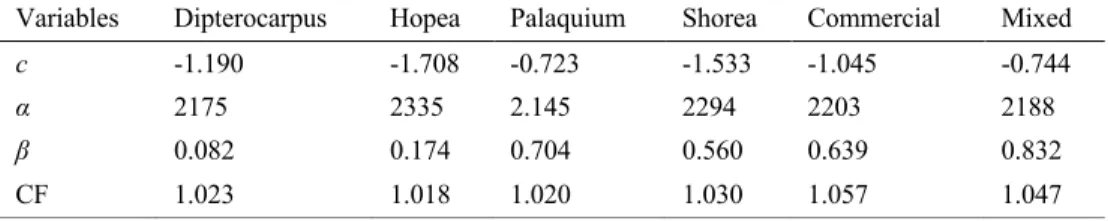
density, and dbh (cm) being the diameter of the tree at breast height (130 cm), intercept (c), slope coefficients (α and β) and correction factor used to back-transform log-transformed data (CF) differed depending on species grouping (Table 3.). I chose to use this equation to estimate TAGB as this equation was derived specifically for moist dipterocarp-dominated rainforests. The wood densities used were collected from the Global Wood Density Database (Chave et al., 2009; Zanne et al., 2009). Species-specific wood densities were used when available and where more than one value existed for the same species; a mean of these values was used. If no species- or genus-specific wood densities were found, a mean of family-genus-specific wood densities was used. TAGB was estimated in total as well as divided by large (≥ 10 cm dbh) and small (10 > x ≥ 5 cm dbh) trees and by species group. The variables (c, α, β and CF) for

Dipterocarpus, Hopea, Palaquium and Shorea were used for their corresponding genus,

while the remaining species in the species group dipterocarps used those of “Commercial” (Table 3.). The species group other commercial used the variables of “Commercial” while the variables of “Mixed” were used for pioneers, fruit trees and unidentified trees (Table 3.).

Table 3. Model variables for Equation 2 (c: intercept, α & β: slope coefficients, CF: correction factor).

Variables Dipterocarpus Hopea Palaquium Shorea Commercial Mixed

c -1.190 -1.708 -0.723 -1.533 -1.045 -0.744

α 2175 2335 2.145 2294 2203 2188

β 0.082 0.174 0.704 0.560 0.639 0.832

CF 1.023 1.018 1.020 1.030 1.057 1.047

• Commercial: mix of four genera; Dipterocarpus, Hopea, Palaquium, Shorea. • Mixed: mix of commercial and non-commercial species

The belowground biomass stored in tree roots and stumps is an important carbon pool which is difficult to estimate by sampling due to methodological complications in terms of observation and measurements (Titlyanova et al., 1999; Vogt et al., 1995). Thus, in addition to determining coarse (> 2 mm) and fine (< 2 mm) root density from soil samples, I also estimated tree belowground biomass (TBGB) by assuming a root : shoot ratio of 0.235 as described in Mokany et al. (2006). There is a potential for overlap in carbon estimates between the collected coarse roots (> 2 mm) and the estimated TBGB (≥ 5 mm) as I could not differentiate between roots belonging to trees or other vegetation. If all collected coarse roots were ≥ 5 mm in diameter as well as all belonging to tree root systems, this overlap would be a maximum of 2% of the total carbon stocks and would therefore be considered negligible.

Liana dry biomass was estimated using the model of Schnitzer et al. (2006): AGB = exp[-1.484 + 2.657 ln(dbh)] (3),

where liana AGB represents the aboveground liana dry biomass (kg/liana) and dbh (cm) the diameter of the liana at breast height (130 cm).

The dry biomass of standing dead wood and woody debris that was too large to weigh was estimated based on volume and wood density using the equations of Chao et al. (2009). Volume of the woody debris was calculated from length and diameter at each end, whereas for the volume of standing dead wood was calculated from height and dhh. For both woody debris and standing dead wood, dry biomass was determined for each decomposition class, in

ρd=1 = 1.17[ρBA j ] − 0.21 (4)

and

ρd=2 = 1.17[ρBA j ] − 0.31 (5),

ρd=1 and ρd=2 represent dead wood density (g cm-3) for class 1 (d=1) and 2 (d=2)

by their basal area. As suggested by Chao et al. (2008), an average wood density value of 0.29 g cm-3 _{was used for all dead wood in decay class 3.}

Soil nutrient- and texture values were calculated using the laboratory results (Table 1.) and soil bulk density (Equation 1.). For easier comparison to other studies, soil nutrient values were scaled to Mg ha-1 _{to 1-meter depth and soil texture values to g cm}-3_.

2.4.2 Tree diversity

To assess tree diversity in each plot, I calculated Shannon´s diversity index, Pielou´s evenness index and rarefied species richness (rarefied to account for varying sample sizes). I also determine these indices for both large (≥ 10 cm dbh) and small trees (10 > x ≥ 5 cm dbh) using the R package “vegan” (v2.5-5; Oksanen et al., 2019). Shannon´s diversity index (Peet, 1974);

@´ = − C 2_Dlog 2_D (6)

I DJK

Where @´ is the diversity index value, S the species richness (rarefied; Equation 8.) and

pi the proportion of individuals belonging to the ith species in the dataset. Pielou´s

evenness index (Hill, 1973); L´ = @´

@´MNO (7)

Where L´ is the evenness index value, @´ the value derived from Shannon´s diversity index and @´_MNO the maximum possible value of @´. Rarefaction of species richness (Hurlbert, 1971); -QR= C(1 − SD) I DJK , where SD = YZ[O\ R ] YZ_R] (8)

Where the expected number of species in a sample is rarefied from N to n individuals, -Q_R is the rarefied species richness, S the species, xi the number of species i, YZ_R] the

binomial coefficient which determines how many ways n can be chosen from N and finally qi gives the probabilities that species i does not appear in a sample size of n.

2.4.3 Statistical analysis

One-way ANOVA was used to test for differences for variables between treated plots and untreated control for carbon density in total, by carbon pool and by functional

species group for both large and small trees. To assess the effects of restoration treatment, linear regressions were performed to test for correlation of diversity indices, carbon density in total, by carbon pool and by functional species group for both large and small trees over time since planting for the nine treated plots combined. Linear regressions were also performed to test for influence of soil edaphic factors on living and dead AGC and on stem density of large and small trees. A significance threshold of p < 0.05 was used and backwards elimination was performed until a minimum adequate model was reached. All calculations and statistical analyses were performed using the R statistical software version 1.2.1335 (R Core Team, 2019).

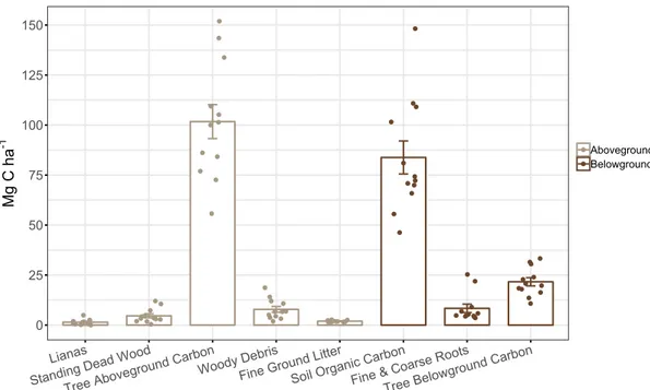
Figure 4. Bar plot of above- (grey) and belowground (brown) carbon pools (Mg C ha-1_{) (± SE) of a}

secondary tropical forest in Sabah Borneo. Small dots represent the plot values from all 12 plots, regardless of time since restoration.

There were no significant differences between total carbon density or the various carbon pools and time since planting. Therefore, I combined the carbon density values from all 12 plots to show the overall carbon budget of a secondary lowland dipterocarp forest 35 years after disturbance (Figure 4.). When combining the carbon density values for all 12 plots, I estimated a mean carbon density (± SE) of 231.4 ± 11.2 Mg C ha-1_{. This}

includes both the aboveground: tree aboveground carbon (TAGC: 44.0%, 101.7 ± 8.5 Mg C ha-1_{), woody debris (3.4%, 7.9 ± 1.5 Mg C ha}-1_{), standing dead wood (2.0%, 4.5}

0 25 50 75 100 125 150 Lianas Standing D ead Wood Tree Above ground Carb on Woody Deb ris Fine Grou nd Litter Soil Organi c Carbon

Fine & Coarse Roots Tree Below ground Carb on Carbon Pools Mg C h a -1 _Aboveground Belowground

3 Results

± 1.0 Mg C ha-1_{), fine litter (FGL: 0.8%, 2.0 ± 0.1 Mg C ha}-1_{), and lianas (0.6%, 1.4 ±}

0.4 Mg C ha-1_{) and belowground: soil organic carbon to 1 meter depth (SOC: 36.2%,}

83.8 ± 8.2 Mg C ha-1_{), tree belowground carbon (TBGC: 9.3%, 21.6 ± 2.1 Mg C ha}-1_),

fine & coarse roots (3.6%, 8.4 ± 2.1 Mg C ha-1_{) carbon pools (Figure 4.).}

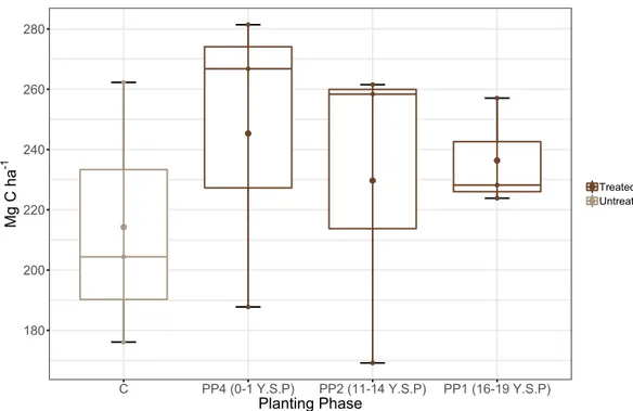
Figure 5. Box plot of total carbon in a degraded tropical forest (grey) as well as within areas of assisted

regeneration with enrichment line planting (brown). Enrichment line planting has occurred in three distinct planting phases (PP) which represents different ages since restoration. Y.S.P denotes approximate years since planting in the different planting phases whereas C represent untreated control plots. Small dots indicate plot values (n = 3 plots per planting phase and control).

Overall, total carbon density, which includes both above- and belowground carbon pools, ranged between 169.2 and 281.4 Mg C ha-1 _{(Figure 5.). Although not a}

significantly different (p > 0.05), total carbon density in treated plots was 10% greater than untreated control plots (237.1 and 214.3 Mg C ha-1_{; respectively) with TAGC and}

SOC making up a large portion of that difference (10 Mg C ha-1 _{and 13 Mg C ha}-1_;

respectively). 180 200 220 240 260 280

C PP4 (0-1 Y.S.P) PP2 (11-14 Y.S.P) PP1 (16-19 Y.S.P) Planting Phase Mg C h a -1 Treated Untreated

Figure 6. Linear regressions of carbon densities (Mg C ha-1_{) in the different carbon pools measured in this}

study over time since planting. Control plot values were not used in the regressions and are shown as hollow symbols as a reference. Y.S.P denotes approximate years since planting in the different planting phases whereas C represent untreated control plots.

For different carbon pools, there was no significant relationship between the amount of carbon stored in aboveground trees, standing dead wood, lianas, soil, woody debris, fine ground litter, belowground trees and fine & coarse roots and time since planting (Figure 6.). However, there is a marginally significant decrease in in carbon density in standing dead wood with time since restoration (Figure 6B.), corresponding to a reduction of ~4 Mg C ha-1 _{in recently treated plots compared to plots that were treated > 15 years ago.}

Tree Aboveground Carbon

Y.S.P Mg C h a -1 C 0 5 10 15 20 0 30 60 90 120 150 R2_{= -0.143} p = 0.98 A

Standing Dead Wood

Y.S.P Mg C h a -1 C 0 5 10 15 20 0.0 2.4 4.8 7.2 9.6 12.0 R2_{= 0.31} p = 0.069 B Lianas Y.S.P Mg C h a -1 C 0 5 10 15 20 0 1 2 3 4 5 R2_{= -0.138} p = 0.86 C

Soil Organic Carbon

Y.S.P Mg C h a -1 C 0 5 10 15 20 0 30 60 90 120 150 R2_{= -0.0639} p = 0.49 D Woody Debris Y.S.P Mg C h a -1 C 0 5 10 15 20 0 4 8 12 16 20 R2 = -0.102 p = 0.63 E

Fine Ground Litter

Y.S.P Mg C h a -1 C 0 5 10 15 20 0.0 0.6 1.2 1.8 2.4 3.0 R2 = -0.0241 p = 0.4 F

Fine & Coarse Roots

Y.S.P Mg C h a -1 C 0 5 10 15 20 0 5 10 15 20 25 R2 = 0.047 p = 0.28 G

Tree Belowground Carbon

Y.S.P Mg C h a -1 C 0 5 10 15 20 0 7 14 21 28 35 R2 = -0.141 p = 0.92 H

Figure 7. Box plots of carbon density (Mg C ha-1_{) and stem density (stems ha}-1_{) in large (≥ 10 cm dbh; A,}

B) and small (10 > x ≥ 5 cm dbh; C, D) trees among the four functional species groups (dipterocarps, other

commercial, fruit trees and pioneers) in a degraded tropical rainforest in Borneo. Small dots represent the

plot values from all 12 plots, regardless of time since restoration. Error bars represent a 95% confidence interval.

Carbon and stem densities for the dipterocarp, fruit tree, and other commercial functional species groups did not show any significant difference over time since planting or between treated- and control plots. Combining the carbon and stem density values for the functional species groups of all 12 plots through large and small trees provides an overview of the forest structure in the sampled plots (Figure 7.). Of the large trees of the functional species groups, those belonging to the dipterocarps contributed roughly 7 times more to total carbon density than those of the fruit trees (Figure 7A.). The mean carbon density of large fruit trees in planting phase 1 (8.2 ± 1.1 Mg C ha-1₎

and planting phase 2 (8.0 ± 0.9 Mg C ha-1_{) was approximately twice as high as the mean}

carbon density of fruit trees in the untreated control (4.5 ± 0.8 Mg C ha-1_).

0 15 30 45 60 75 Dipteroca rps Other Co

mmercial_Fruit Trees Pioneers

Mg C h a -1 Carbon Density (≥ 10 cm dbh) A 0 65 130 195 260 325 Dipteroca rps Other Co

mmercial_Fruit Trees Pioneers

St ems ha -1 Stem Density (≥ 10 cm dbh) B 0 3 6 9 12 15 Dipteroca rps Other Co

mmercial_Fruit Trees Pioneers

Mg C h a -1 Carbon Density (5 ≤ x < 10 cm dbh) C 0 200 400 600 800 1000 Dipteroca rps Other Co

mmercial_Fruit Trees Pioneers

St ems ha -1 Stem Density (5 ≤ x < 10 cm dbh) D

Figure 8. Linear regressions of carbon density (A) and stem density (B) for large (≥ 10 cm dbh) pioneers

over time since planting. Data from control plots were excluded from the regression analyses and are shown (hollow symbols) only for reference.

There are many pioneer trees (Figure 7B.) but they contribute to a low fraction of the overall carbon density (Figure 7A.). For large pioneer trees there was a drastic decrease in carbon- and stem density after treatment and a significant positive relationship between time since planting and carbon density (p < 0.01; Figure 8A.) and stem density (p < 0.01; Figure 8B.) for the treated plots. For small trees, both carbon (4.8 ± 1.3 Mg C ha-1_{) and stem density (445.8 ±105.4 stems ha}-1_{) was highest for pioneer trees (Figure}

7C, D.).

Pioneer Carbon Density (≥ 10 cm dbh)

Years Since Planting

Mg C h a -1 C 0 5 10 15 20 0 6 12 18 24 R2 = 0.75 p = 0.0016 A

Pioneer Stem Density (≥ 10 cm dbh)

Years Since Planting

St ems ha -1 C 0 5 10 15 20 0 70 140 210 280 R2 = 0.693 p = 0.0033 B

Figure 9. Linear regressions of Shannon´s diversity index (A and D), Pielou´s evenness index (B and E)

and rarefied species richness (C and F) over time since planting for large (≥ 10 cm dbh; A-C) and small (10 > x ≥ 5 cm dbh; D-F) trees. Control plot values were not used in the regressions and are shown as hollow symbols as a reference.

No significant differences were detected for any of the diversity indices (Shannon´s diversity, Pielou´s evenness and rarefied species richness) over time since planting for the treated plots (p > 0.05), either for large (≥ 10 cm dbh) or for small (10 > x ≥ 5 cm dbh) trees (Figure 9.).

Diversity (≥ 10 cm dbh)

Years Since Planting

Sh an no n´s D ive rsi ty C 0 5 10 15 20 0 1 2 3 4 R2 = -0.127 p = 0.76 A Evenness (≥ 10 cm dbh)

Years Since Planting

Pi el ou ´s Eve nn ess C 0 5 10 15 20 0.00 0.02 0.04 0.06 0.08 0.10 R2 = 0.113 p = 0.2 B Species Richness (≥ 10 cm dbh)

Years Since Planting

R are fie d Sp eci es R ich ne ss C 0 5 10 15 20 0 11 22 33 44 55 R2 = -0.132 p = 0.8 C Diversity (10 > x ≥ 5 cm dbh)

Years Since Planting

Sh an no n´s D ive rsi ty C 0 5 10 15 20 0 1 2 3 4 R2 = -0.086 p = 0.56 D Evenness (10 > x ≥ 5 cm dbh)

Years Since Planting

Pi el ou ´s Eve nn ess C 0 5 10 15 20 0.0 0.2 0.4 0.6 0.8 1.0 R2 = -0.133 p = 0.81 E Species Richness (10 > x ≥ 5 cm dbh)

Years Since Planting

R are fie d Sp eci es R ich ne ss C 0 5 10 15 20 0 3 6 9 12 15 R2 = 0.0579 p = 0.26 F

Figure 10. Box plot of carbon density (A) and stem density (B) of large (≥ 10 cm dbh) and small (10 > x ≥

5 cm dbh) planted trees in the two oldest planting phases (PP). Y.S.P denotes approximate year since planting in the different planting phases.

Only in planting phases 1 and 2 (> 10 Y.S.P), were the planted trees now larger than 5 cm in diameter. The carbon density for planted trees lies between 0 and 2.5 Mg C ha-1

with large carbon density observed in older treated plots (i.e., PP1; Figure 10A.). Similarly, stem density of planted trees was larger in the older treated plots and ranged between 0 and 200 stems ha-1_{. It is worth pointing out that in PP1 I observed a lower}

stem density of large (≥ 10 cm dbh) compared to small (10 > x ≥ 5 cm dbh) trees, yet these larger trees contributed more to the total carbon density. Despite these trends, the contribution of planted trees to TAGC in planting phase 1 (16-19 Y.S.P) was 1.07% for large and 0.74% for small trees, whereas stem density was 2.35% and 7.83% per cent of total stem density for planted large and small trees respectively. For planting phase 2 (11-14 Y.S.P), the contribution of planted trees to TAGC was 0% and 0.09% for large and small trees, and their contribution to total stem density was 0% and 1.05% for planted large and small trees, respectively.

0.0 0.5 1.0 1.5 2.0 2.5 PP2 (11-14 Y.S.P) PP1 (16-19 Y.S.P) Planting Phase Mg C h a -1 Carbon Density A 0 40 80 120 160 200 PP2 (11-14 Y.S.P) PP1 (16-19 Y.S.P) Planting Phase St ems ha -1 Planted Trees 5 ≤ x < 10 cm dbh ≥ 10 cm dbh Stem Density B

Figure 11. Linear regressions between soil clay (<0.002 mm; A), silt (0.002 – 0.06 mm; B) and sand (0.06

- 2 mm; C) content and living and dead AGC. Living AGC (blue) represent carbon density in both trees and lianas, whereas dead AGC (yellow) represent the carbon density of woody debris, fine ground litter and standing dead wood.

When combining all 12 plots together, I observed a significant negative relationship between the carbon density in living AGC and silt content (p < 0.01; Figure 11B.). Whereas, the relationship of carbon density in living AGC over sand content and of dead AGC over clay content was only marginally significant (p < 0.1; Figure 11A, C.). More silt in the soil appeared to be a strong indicator (R2 _{= 0.51) for decreased living}

AGC in a plot, with a difference of over 90 Mg C ha-1 _{between the plots with the highest}

and lowest silt density (0.54 g cm-3 _{and 0.18 g cm}-3_{; respectively).}

R^2 = 0.21, p = 0.078 0 50 100 150 0.2 0.3 0.4 0.5 0.6 g cm-3 Mg C h a -1 Clay A R^2 = 0.51, p = 0.0052 0 50 100 150 0.2 0.3 0.4 0.5 g cm-3 Mg C h a -1 Silt B R^2 = 0.26, p = 0.052 0 50 100 150 0.2 0.4 0.6 0.8 g cm-3 Mg C h a -1 AGC Living Dead Sand C

Figure 12. Linear regressions between soil phosphorus (A), nitrogen (B) and carbon (C) and stem density

in small (blue) and large trees (yellow) in all 12 plots. Soil texture particle sizes: clay (<0.002 mm), silt (0.06 - 0.002 mm) and sand (2 - 0.06 mm).

I performed linear regressions for the stem densities of large and small trees over soil characteristics for all 12 plots; soil nutrients (Figure 12A-C.) and soil textures (Figure 12D-F.). Of the regressions for stem densities over soil nutrients, two correlations have shown to be significant; stem density of small trees over phosphorus density (p < 0.05; Figure 12A.) and stem density of large trees over nitrogen density (p < 0.05; Figure 12B.). Of the regressions for stem densities over soil texture only one has shown to be significant; stem density of large trees over silt density (p < 0.05; Figure 12E.). Aside from the significant correlations, there appears to exist emergent trends for stem densities of small trees over silt density, and for large trees over carbon, clay, and sand density as well (Figure 12C-F.). Further analysis revealed that, stem density of large trees (≥ 10 cm dbh) of the functional species group: pioneers, was found to significantly correlate with phosphorus density (R2 _{= 0.64, p = 0.001).}

R^2 = 0.44, p = 0.011 0 500 1000 1500 2 3 4 5 Mg C ha-1 St ems ha -1 Phosphorus A R^2 = 0.34, p = 0.028 0 500 1000 1500 10 15 20 Mg C ha-1 St ems ha -1 Nitrogen B R^2 = 0.19, p = 0.087 0 500 1000 1500 50 75 100 125 150 Mg C ha-1 St ems ha -1 Carbon C R^2 = 0.23, p = 0.064 0 500 1000 1500 0.2 0.3 0.4 0.5 0.6 g cm-3 St ems ha -1 Clay D R^2 = 0.25, p = 0.058 R^2 = 0.43, p = 0.013 0 500 1000 1500 0.2 0.3 0.4 0.5 g cm-3 St ems ha -1 Silt E R^2 = 0.21, p = 0.074 0 500 1000 1500 0.2 0.4 0.6 0.8 g cm-3 St ems ha -1 Sand F 5 ≤ x < 10 cm dbh ≥ 10 cm dbh

This study is unique in that I quantified both above- and belowground carbon stocks (including soil carbon) within 12 plots to get a more accurate estimate of the total C balance in a secondary lowland dipterocarp rainforest in Borneo. Additionally, measurements were made in control plots and restoration plots that consist of enrichment line planting. There appeared to be a 10% (~20 Mg C ha-1_{) increase in total}

carbon density in the treated compared to the untreated control plots, although the difference was not statistically significant. The restoration method of enrichment line planting showed no improvement on tree diversity, yet more time and research effort may be needed to properly assess if this restoration method has a positive effect on tree diversity.

Few studies have directly measured both above- and belowground carbon stocks in dipterocarp rainforests. Instead, the majority of previous studies have focused on aboveground biomass, which limits our understanding of the total carbon budget in these forests. When combining all 12 plots, mean (± SE) total carbon density was 231.4 ± 11.2 Mg C ha-1_{. The two major carbon pools; tree aboveground carbon (TAGC; 101.7}

± 8.5 Mg C ha-1_{) and soil organic carbon (SOC; 83.8 ± 8.2 Mg C ha}-1_{) together store}

80% of the total ecosystem carbon, whereas the remaining carbon pools (i.e., woody debris, FGL, standing dead wood, lianas, TBGC and fine & coarse roots), when aggregated, accounted for the remaining 20% of the total ecosystem carbon (45.9 ± 2.2 Mg C ha-1_{; Figure 4.). Interestingly, I found that belowground carbon pools represented}

roughly half (49%) of the total carbon budget, which is in contrast to other studies in the area that have reported only one-third of the total carbon is found belowground (Saner et al., 2012; Hector et al., 2011).

The primary objective of the INIKEA project was to use assisted regeneration by enrichment line planting and liberation accelerate secondary succession thereby promoting biodiversity and restoring degraded, secondary forests to their original

4 Discussion

structure. In this study the main focus was on examining the effects of enrichment line planting on total ecosystem carbon balance. Other studies have reported positive effects on forest structure and growth for both enrichment line planting and liberation (Schnitzer et al., 2014; Karam et al., 2012; Kuusipalo et al., 1996; Ådjers et al., 1995). In this study, I found no significant change in above- and belowground carbon stocks in total or by carbon pool in response to enrichment planting (Figure 5-6.). Additionally, the mean carbon density of planted seedlings (≥ 5 cm dbh) in the plots of planting phase 1 (16-19 Y.S.P) was estimated to 2 Mg C ha-1 _{(Figure 10.), which corresponds to ~2%}

of TAGC. However, it is important to point out that carbon density was ~20 Mg C ha-1

(10%) greater in the treated compared to the untreated control plots. Albeit this difference was not significant, it remains possible that the limited number of plots made significance difficult to attain. This apparent increase in total carbon density was partly the result of greater TAGC and SOC in the treated compared to untreated plots (10 and 13 Mg C ha-1 _{higher; respectively). To reduce the uncertainty due to soil edaphic}

properties and the spatial variation inherent to the study site, a greater number of plots would be needed in both treated as well as untreated control areas. To examine this possibility, I performed a t-test power analysis with a power level of 0.8 as described in Cohen (1988), which showed that given the variation and 10% difference in treatments a sample size of n=33 would have been needed to detect a significant difference in total carbon stocks between control plots and planting phase 1 plots. Thus, it appears that assisted enrichment planting may have a positive effect on the total C pools of degraded lowland dipterocarp forests, yet further studies are needed to better assess the potential of enrichment line planting in restoring secondary tropical rainforests in terms of carbon sequestration.

Several studies have shown that soil edaphic properties (e.g. soil texture) can influence aboveground forest structure (e.g. aboveground biomass, species composition, etc.) in tropical rainforests (Paoli et al., 2008; Clark et al., 1999; Laurance et al., 1999), which in part may help explain the large variation, and thus contributed to the difficulty to assess statistical differences. I found that soil edaphic properties, namely soil texture and both soil nitrogen and phosphorus, influences stem density and living aboveground carbon (Figure 7, 8). These findings, coupled with the well documented spatial variability of tropical rainforests (Saatchi et al., 2011; Clark & Clark, 2000), could help explain why the applied treatment of enrichment line planting and liberation did not significantly enhance carbon sequestration in my study. Furthermore, it is important to remember that the main objective of the INIKEA project was to enhance biodiversity, and if the carbon sequestration was the main objective then a different suite of seedlings might have been used which, in turn, may have resulted in larger carbon sequestration in treated plots. However, restoration practices with the sole intent of increased carbon

sequestration can, in some cases, have adverse effects on biodiversity, natural forest structure and ecosystem services through the homogenization of the landscape (Edwards et al., 2010a; Putz & Redford, 2009)

There are several different allometric equations for estimating aboveground biomass in tropical forests (Chave et al., 2014; Basuki et al., 2009; Chave et al., 2005; Brown, 1997). I used the equations described in Basuki et al. (2009) as they were developed specifically for lowland dipterocarp forests and was thus was the most appropriate for my study. The choice of allometric equations is an important one as they can differ greatly between each other which can therefore reduce the accuracy of comparisons (Feldpausch et al., 2011; Henry et al., 2010; Houghton et al., 2001). For example, it has been shown that aboveground biomass is often underestimated when using the models of Basuki et al. (2009) relative to those of other studies. However, I decided to use the Basuki model since site-specific equations generally improve biomass estimates when applied to the area they are developed for (Huy et al., 2016; Paul et al., 2016; Ngomanda

et al., 2014; Kenzo et al., 2009; Segura & Kanninen, 2005; Cairns et al., 2003). Another

potential source of uncertainty in my estimates of TAGC may be related to the problem that approximately 8% of the trees included in this study were unidentified at species, genus or family level. However, due to the relatively low number of unidentified trees and the fact that I used plot-average wood density for these unidentified trees, this likely resulted in a relatively minor impact on the estimates of TAGC.

When assessing the impact of treatment on overall tree diversity, no significant effect (p < 0.05) was found on “desired” functional species groups or diversity indices (Shannon´s diversity, Pielou´s evenness, rarefied species richness). Budiharta et al. (2014a) and Schwartz et al. (2013) suggests that the greatest effect of enrichment line planting is observed in highly degraded areas where natural regeneration is lacking. Within the INIKEA project, there is often an abundance of small trees in the understory (Figure 7D.) and several trees > 50 cm dbh. Thus, the sampled plots do not appear to be severely degraded, which might have happened by chance due to the relatively limited number of plots. Therefore, the results of my study might not reflect the situation in the more degraded forests. To raise the effectiveness of the enrichment planting, it would be advantageous to increase efforts to determine the level of degradation in target areas prior to treatment, either by manual survey or by remote sensing techniques (Budiharta

et al., 2014b; Ioki et al., 2014; Kronseder et al., 2012). The increase of pioneer trees

over time since planting (Figure 8.) may, in part, be due to the cutting of lianas and opening up of the canopy as part of the liberation, thereby creating suitable conditions for the growth of pioneer trees (Primack & Lee, 1991). Alternatively, this increase could be a natural recovery for the pioneer trees after having been reduced compared to the

control plots. Yet another possibility is that the availability of soil nutrients, primarily phosphorus, influences the prevalence of pioneer trees as shown by the findings of Raaimakers and Lambers (1996). This would also be supported by my findings as phosphorus density was found to correlate positively with large pioneer tree stem density (p < 0.01). Trees belonging to “undesired” species, such as Macaranga spp., are subject to selective removed during site preparation or subsequent maintenance as shade-adjustment (see experimental design). To ensure that the prevalence of pioneer trees in treatment areas is kept to a minimum, more thorough removal of them over a longer period of time might be necessary. Currently, plot maintenance, which includes the removal of pioneer species, is done for 10 Y.S.P, but it might need to be extended for another 10 years. Especially so as pioneer trees, Macaranga spp. in particular, have been found to limit the recruitment of dipterocarp seedlings (Aoyagi et al., 2013). Lastly, while at the date of sampling, 19-year-old plots since planting were the oldest available in the INIKEA project area, this may be too small an amount of time to observe any significant change in forest structure from the planted seedlings.

Table 4. Carbon stocks and sequestration in tropical primary and secondary dipterocarp forests as well as in timber and oil palm plantations.

Study site Forest type Description Mean SOC _{(Mg C ha}-1₎

Mean TAGC (Mg C ha-1₎ DTAGC (Mg C ha-1 _year-1₎ Diameter limit (cm) Reference

Malaysia Dipterocarp _(Lowland) OS (35 years) 84 102 - ≥ 5 This study

Malaysia Dipterocarp _(Lowland) YS (18 years)

Primary - - 89 138 1.40 0.28 ≥ 5 Berry et al. (2010)

Philippines Dipterocarp OS (≥ 21 years)

Primary 60 65 136 190 1.43 - ≥ 19.5 Lasco et al. (2006)

Malaysia Dipterocarp _(Lowland) OS (≥ 22 years)

Primary 58 - 136 234 - - > 10 Hector et al. (2011) Malaysia Dipterocarp (Lowland) OS (40 years) Primary - - 137* 155* - - ≥ 5 Okuda et al. (2004) Malaysia Dipterocarp (Lowland) OS (22 years) Primary 40 - 92 128 - - > 10 Saner et al. (2012) Indonesia Mixed Dipterocarp OS (55 years) Primary - - 132* 179* - - > 10 Brearley et al. (2004)

Indonesia Oil palm Plantation - 39** 5.85 - Khasanah et _{al. (2015)}

Malaysia Oil palm Plantation

(6-23 years) - 24* - -

Asari et al. (2013)

Brazil Timber (E. globulus _{& E. urophylla)} Plantation

(10 years) 100 118 11.80 -

Viera and Rodríguez-Soalleiro (2019)

Meta-analysis Timber (Inc. Acacia & Eucalyptus spp.) Plantation - 27** 5.00 - Lewis et al. (2019)

Meta-analysis (Asia) Tropical rainforest YS OS Primary - - - - - - 1.70* 1.35* 0.35* - - - Requena Suarez et al. (2019) Lowland = below 500 m a.s.l., Dipterocarp = dipterocarp dominated forest, SOC = soil organic carbon (rounded to nearest integer), TAGC = tree aboveground carbon (rounded to nearest integer), DAGC = aboveground carbon sequestration, YS= young secondary forest (≤20 years), OS = old secondary forest (>20 years), * = values converted to carbon as 50% of original value, ** = time averaged value for 1 rotation period.

Regardless of the impact of enrichment line planting on carbon sequestration and/or overall tree diversity, arguably the most important aspect of an area designated for conservation is that the land will be protected from land-use conversion. The findings of Morel et al. (2012) showed that between the years 2000 to 2008, the area covered by oil palm plantation in Sabah, Malaysian Borneo increased by 38% and it is likely that this would have happened to the forests within the INIKEA project area had it not been protected under a restoration program, since it is now almost entirely surrounded by such plantations. It has previously been shown that carbon sequestration in plantation forestry (5.85 Mg C ha-1 _year-1_{) and oil palm plantations (5-11.8 Mg C ha}-1 _year-1_{) is}

considerably higher than what is observed in primary (0.28-0.35 Mg C ha-1 _year-1_{) and}

secondary (1.35-1.70 Mg C ha-1 _year-1_{) tropical forests (Table 4.). However, it should}

be remembered that higher carbon sequestration rates of plantations compared to natural forest, come at a cost. The difference in both animal and tree diversity between plantations and even secondary rain forest is massive. For example, the abundance of imperilled bird species is 200 times lower in oil palm plantations compared to adjacent tropical forests (Edwards et al., 2010b; Fitzherbert et al., 2008). Furthermore, although carbon sequestration is higher in plantations compared to forests, the amount of aboveground carbon (i.e., TAGC) is greater in forests compared to plantations (Table 4.). Additionally, there are significant greenhouse gas emissions associated with the clearing of natural forest for land-use conversion to plantation forestry (Miles & Kapos, 2008; Fearnside, 1997). Once a natural forest is cleared, the values it holds, be they ecological or otherwise, are very difficult to reconstruct and the process of recovery to that of something resembling primary forest is unlikely to be either linear or uniform. Structural characteristics (e.g. aboveground biomass) will most likely be recovered before other ecosystem services (e.g. biodiversity). Notions of the time it takes for cleared land to recover to something that resembles primary rainforest vary, but includes estimates ranging from 50 to 500 years (Hughes et al., 1999; Kartawinata, 1994; Brown & Lugo, 1990; Riswan et al., 1985; Knight, 1975) and will depend on many factors, including availability of contiguous seed sources and the degree of initial disturbance (Martin et al., 2013; Brearley et al., 2004). Therefore, regardless of any effect or lack thereof from the restoration treatment in the INIKEA project area, the environmental and ecological contributions of the protection of the forests within its borders from being cleared and converted into oil palm or timber plantation remain highly valuable.

In conclusion, this study provides detailed estimates of both above- and belowground carbon stocks in treated and untreated secondary forests in northern Borneo. Although not significant, there appeared to be a 10% (~20 Mg C ha-1_{) increase in total carbon in}

treated compared to untreated plots. My assessment show that more replication is needed to with sufficient statistical power assess if such difference is significant or not. Additionally, results from this study clearly shows that roughly 50% of total ecosystem carbon in found belowground, which is higher in contrast to previous estimates and highlights the need for further studies to quantify belowground carbon stocks. The main objective of the INIKEA project was to increase biodiversity yet results from this study indicate no change in tree biodiversity between treated and untreated control plots. However, the plots used in this study seem to suggest that the forests were not severely degraded, and thus more time may be needed to assess the effect of enrichment line planting on biodiversity. Lastly, additional studies are needed on the conservation value and restoration potential of degraded tropical rainforests and the findings of this study have helped provide a better understanding of carbon stocks in secondary rainforests that can help design future studies to assess the effectiveness of restoration in tropical forests.