Master Thesis in Statistics and Data Mining
Retrieval of Cloud Top Pressure
Claudia Adok
Division of Statistics and Machine Learning
Department of Computer and Information Science
Examiner Mattias Villani
Contents
Abstract 1 Acknowledgments 3 1. Introduction 5 1.1. SMHI . . . 5 1.2. Background . . . 5 1.3. Previous work . . . 6 1.4. Objective . . . 6 2. Data 9 2.1. Data description . . . 9 2.2. Data preprocessing . . . 11 3. Methods 13 3.1. Sampling methods . . . 133.2. Random forest regression . . . 13
3.3. Recursive feature elimination with random forest regression . . . 15
3.4. The multilayer perceptron . . . 16
3.4.1. Mini-batch stochastic gradient descent . . . 18
3.5. Performance evaluation metrics . . . 19
3.6. Technical aspects . . . 20
4. Results 21 4.1. Recursive feature elimination with random forest regression . . . 22
4.2. Random forest regression . . . 23
4.2.1. Results using simple random sampling . . . 24
4.2.2. Results using stratified random sampling . . . 32
4.2.3. Results using simple random sampling on filtered data . . . . 33
4.2.4. Results using stratified random sampling on filtered data . . . 34
4.3. The multilayer perceptron . . . 37
4.3.1. Results using simple random sampling . . . 38
4.3.2. Results using stratified random sampling . . . 43
4.3.3. Results using simple random sampling with a log transformed 45 4.3.4. Results using stratified random sampling with a log transformed 48 4.3.5. Results using simple random sampling on filtered data with a log transformed response . . . 51
4.3.6. Results using stratified random sampling on filtered data with a log transformed response . . . 53 4.4. Comparison of the multilayer perceptron and random forest model . . 59
5. Discussion 61
6. Conclusions 65
Bibliography 67
Abstract
In this thesis the predictive models the multilayer perceptron and random forest are evaluated to predict cloud top pressure. The dataset used in this thesis contains brightness temperatures, reflectances and other useful variables to determine the cloud top pressure from the Advanced Very High Resolution Radiometer (AVHRR) instrument on the two satellites NOAA-17 and NOAA-18 during the time period 2006-2009. The dataset also contains numerical weather prediction (NWP) variables calculated using mathematical models. In the dataset there are also observed cloud top pressure and cloud top height estimates from the more accurate instrument on the Cloud-Aerosol Lidar and Infrared Pathfinder Satellite Observation (CALIPSO) satellite. The predicted cloud top pressure is converted into an interpolated cloud top height. The predicted pressure and interpolated height are then evaluated against the more accurate and observed cloud top pressure and cloud top height from the instrument on the satellite CALIPSO.
The predictive models have been performed on the data using different sampling strategies to take into account the performance of individual cloud classes prevalent in the data. The multilayer perceptron is performed using both the original response cloud top pressure and a log transformed repsonse to avoid negative values as output which is prevalent when using the original response. Results show that overall the random forest model performs better than the multilayer perceptron in terms of root mean squared error and mean absolute error.
Acknowledgments
I would like to thank the Swedish Meteorological and Hydrological Institute (SMHI) for giving me the opportunity to work with them and providing the data for this thesis. I would like to give special thanks to my supervisor Nina H˚akansson at SMHI for providing good support during this work.
I would also like to thank my supervisor Anders Nordgaard for his great advice and support during each stage of the thesis.
Finally, I would like to thank my opponent Zonghan Wu for reviewing my thesis and giving valuable improvement suggestions.
1. Introduction
1.1. SMHI
The commissioner of this thesis is the research group for atmospheric remote sensing at the Swedish Meteorological and Hydrological Institute (SMHI). The research group for atmospheric remote sensing researches cloud and precipitation retrieval using satellite and radar measurements.
1.2. Background
Data collected from imager-instruments on satellites are used in weather forecasting. The cloud top pressure and cloud top height gives valuable information on current weather situations. Information about cloud top height is important for preparation of weather forecasts as well as climate monitoring. Cloud top height is difficult to derive from satellite data.
Classical approaches to calculate cloud top height nowadays like optimal estimation and arch fitting are slow for short-term weather forecasts and when reprocessing large datasets within climate research. Scientific knowledge about the atmosphere is currently what is used for weather forecasting. The unreliable nature of the atmo-sphere and the lack of understanding all the atmospheric processes make machine learning algorithms that are able to solve complex and computational expensive equations appealing.
Artificial neural networks and random forests are predictive models proven to be useful when non-linear relations are present which is the case in weather forecasting. The artificial neural networks arise from the idea of the human brain and the neurons of the human brain. The fact that artificial neural networks can learn by example make them useful for forecasting when a lot of data is available. Neural networks have proven to be an excellent machine learning algorithm not only in the field of atmospheric sciences but also in other fields such as finance and medicine.
Random forest is a non-linear statistical method that grows an ensemble of de-correlated regression trees. Random forest is known to have good predictive power when trained on a lot of data as well as being robust to outliers, which is appealing in weather forecasting.
1.3. Previous work
Machine learning algorithms have been used in the field of atmospheric science for various purposes. In Naing and Htike [18] random forests were used to forecast monthly temperature variations in Kuala Lumpur based on time series data gath-ered from year 2000 to 2012. Temperature variations are important for climate monitoring, agriculture and various other reasons. The random forest model was used for forecasting of minimum and maximum temperature for one month ahead. In the paper the random forest model was compared to other machine learning methods, one of them being the multilayer perceptron. The random forest model showed better results in terms of prediction accuracy of minimum and maximum temperature than other machine learning methods used in the comparison.
In Kolios et al. [12] the multilayer perceptron is used to predict cloud top height on a pixel basis by using Meteosat Second Generation water vapory images. As a reference dataset radiosonde measurements were used. The authors focused on predicting the cloud top height of optically thick clouds that are important for anticipating severe weather conditions. In the paper a multilayer perceptron with one hidden layer as well as a multilayer perceptron with two hidden layers were evaluated and gave promising results.
In Kuligowski and Barros [13] a backpropagation neural network is used to forecast 6-h precipitation forecasts for specific locations. Results showed that the neural net-work with its ability to detect non-linear relations gave better results than ordinary linear regression for moderate to heavier precipitation events. Forward screening regression was used to perform variable selection. A neural network with a sigmoid transfer function for the hidden layer and no activation function for the output layer was used.
In Hayati and Mohebi [10] artificial neural networks have proven to be useful for short-term temperature forecasting. The type of neural network used for forecasting was a multilayer perceptron with three layers trained on 10 years of past data. It was used for one day ahead forecasting of temperature of Kermanshah city located in west Iran. The performance of the model was good in terms of the performance metric mean absolute error and showed to be a promising model for temperature forecasting.
1.4. Objective
In this thesis I will predict cloud top pressure using neural networks. An alternative method to predict cloud top pressure besides neural networks will also be used and the two methods will be compared. The data used to predict cloud top pressure is satellite data from the imager-instrument Advanced Very High Resolution Radiome-ter (AVHRR) as well as numeric weather prediction (NWP) variables. The predicted
1.4 Objective
cloud top pressure will be converted to an interpolated cloud top height using a for-mula. Tbe predicted cloud top pressure and interpolated cloud top height will then be compared to the observed cloud top pressure and cloud top height from the more accurate instrument on the satellite CALIPSO. Different performace metrics will be used to evaluate the performance of the two predictive methods.
2. Data
2.1. Data description
The dataset contains brightness temperatures, reflectances and other useful vari-ables to determine the cloud top pressure from the imager-instrument AVHRR on the two satellites NOAA-17 and NOAA-18 during the time period 2006-2009. The dataset also contains numerical weather prediction (NWP) variables calculated us-ing mathematical models. In the dataset there are also observed cloud top pressure and cloud top height estimates from the more accurate instrument on the satellite CALIPSO. For some variables where a lot of missing values were prevalent a de-fault value decided from scientific knowledge of those specific variables was used for those observations. Other observations containing missing values for any variable were removed. After removal of missing values, the dataset has in total 574828 observations. Each observation represents a pixel. The observations in the data can be divided into the three different cloud classes low, medium and high which are derived by an algorithm for the CALIOP-data. CALIOP is the active lidar on the satellite CALIPSO. There are in total 276 variables used as predictors and one response variable. The variables are the following:
Continuous variables: • Azimuth difference
• Brightness temperatures of the 11, 12 and 3.7 micron channel • Emissivity of the 3.7, 11 and 12 micron channel
• Longitude and latitude
• Reflectances of the 0.6 and 0.9 micron channel • The satellite zenith angle
• The solar zenith angle
• Texture of reflectances of the 0.6 micron channel • Texture of different temperatures
• Threshold values for different reflectances and temperatures • Cloud top pressure
• Total optical depth
Continuous numeric weather prediction variables (NWP): • Fraction of land
• Simulated cloud free brightness temperature of the 11 and 12 micron channel measured over land and sea level
• Height for 60 different levels in the atmosphere • Mean elevation
• Pressure for 60 different levels in the atmosphere • Tropopause pressure and temperature
• Surface height
• Surface land temperature • Surface temperature
• Temperature at 500,700,850 and 950 hPa • Pressure at surface level
• Surface sea temperature • Temperature at 850 hPa
• Temperature for 60 different levels in the atmosphere • Column integrated water vapour
Discrete variables: • Cloud type
• Cloud type conditions • Cloud type quality • Cloud type status
Variables used for conversion from cloud top pressure to interpolated cloud top height:
• Height and pressure at different levels in the atmosphere • Surface pressure and surface height
Variables used for dividing the observations into cloud classes: • Number of cloud layers
2.2 Data preprocessing
The response variable describing cloud top pressure and the variable describing cloud top height is measured with the more accurate instrument on the satellite CALIPSO. The variables describing cloud top height and total optical depth are not among the predictors used in the thesis.
The pressure, temperature and height for 60 different levels in the atmosphere are treated as 60 different variables, one variable for each level. Only 36 out of the 60 variables representing pressure at different levels are used as predictors since the last 14 variables has the same value for each observation and are therefore not useful as predictors.
The difference between the brightness temperature of the 11 and 12 micron channel is also added as a variable to the dataset.
2.2. Data preprocessing
The four discrete variables describing cloud type, cloud type conditions, cloud type quality and cloud type status were transformed with one hot encoding into as many dummy variables as there are categories for each variable. This is necessary since otherwise the neural network and random forest model will interpret these variables as numeric which they are not since the categories of these variables do not have any specific order. Standardization of data in neural networks is important and makes the training of the network faster as well as helps prevent the neural network to get stuck in a local minimum and helps ensure convergence. In random forests however there is no need to standardize the data. The inputs and outputs of the neural network model were standardized to have mean 0 and standard deviation 1 by using the formula:
z = x − µ
σ (2.1)
where µ is the mean and σ is the standard deviation of a variable in the training data.
3. Methods
3.1. Sampling methods
Different sampling methods have been used before splitting the data into training, validation and test data. All data or only part of the data was sampled using both simple random sampling and stratified random sampling.
A filtered dataset with observations where the total optical depth is larger than the threshold value 0.5 was also used as data. The filtered data was used to see if the performance of the neural network model and random forest model would improve once observations for thinner clouds which can be hard to detect by an instrument were removed.
When cross-validation is used for parameter tuning for the two predictive models in the thesis, 100 000 observations are sampled using simple random sampling and the observations are then split into data used for cross-validation and test data. 80% of the sampled data is used for cross-validation and 20% as test data. When using simple random sampling on all the data, the observations were randomly sampled and 50% of the observations were used as training data, 25% of the observations as validation data and the remaining 25% as test data. When using stratified random sampling the data is divided into different subgroups and observations are randomly selected from each subgroup according to some sample size. The stratified random sampling was based on the three different cloud classes low, medium and high derived by an algorithm for the CALIOP-data. Two strategies, one where an equal amount of observations was sampled from each cloud class and the other where a higher amount of observations being sampled from the low cloud class was used. 50% of the sampled observations from each cloud class were used as training data, 25% of the observations as validation data and the remaining 25% as test data. The same data splitting into training, validation and test data is used for the two predictive models in the thesis when the same sampling method is used.
3.2. Random forest regression
The non-linear statistical method random forest was chosen as one of the methods to predict cloud top pressure in this thesis because of its many advantages such as that it’s known to have good predictive power when trained on a lot of data as well
as being robust to outliers. Random forest regression is a method that constructs several regression trees. When there is a split in a tree a random set of variables are chosen from all the variables. By doing this one avoids the predictions from the trees having high correlation, since the most important variable will not always be used in the top split in the trees. The algorithm for random forest regression is [9]:
Algorithm 2.1 Random forest regression
1. For b = 1 to B:
(a) Sample N observations at random with replacement from the training data
(b) Grow a random forest tree Tb to the sampled N observations, by recursively
repeating the following steps for each terminal node of the tree, until a minimum node size nmin is reached
i. Select m variables at random from the p variables
ii. Select the best variable/split-point among the m variables iii. Split the node into two daughter nodes
2. Output the ensemble of trees {Tb} B 1
The following formula is used to make a prediction at a new point x: ˆ frfB(x) = 1 B B X b=1 Tb(x)
Parameters to tune when performing random forest regression are the number of trees, the number of variables selected at each split and the maximum depth of the trees. These three parameters were tuned by performing a grid search with 3-fold cross-validation and the model chosen is the model with the average minimum mean squared error (MSE). Random forest is robust to overfitting because of the randomness in the trees in the algorithm. When building a random forest model N observations are sampled at random with replacement, a method called boot-strapping, the observations not selected by the model are called out of bag samples. Because of each tree being built on a bootstrapped dataset and a number of vari-ables are selected at random at each split in the tree the random forest algorithm is more unlikely to overfit than if a simple regression tree would have been used.
3.3 Recursive feature elimination with random forest regression
3.3. Recursive feature elimination with random forest
regression
Recursive feature elimination (RFE) with random forest regression is a variable se-lection method which uses a backward sese-lection algorithm and the measure variable importance calculated by the random forest model to determine which variables to eliminate in each step. The recursive feature elimination starts out with all vari-ables and fits a random forest model and calculates the variable importance for each variable to determine the ranking of the variables. For each subset size used in the algorithm the most important variables are kept and a new random forest is fit with the kept variables. The performance of the subset is measured by the root mean squared error (RMSE). To take into account the variation in the performance estimates as a result of the variable selection, 3-fold cross-validation is used as an outer resampling method. The chance of overfitting the predictors is diminished by using cross-validation. When using 3-fold cross-validation two-thirds of the data will be used to perform the variable selection while one–third of the data is used as a held-back set and will be used to evaluate the performance of the model for each subset of variables. The variable selection process will thus be performed three times using a different hold-out set each time. The optimal number of variables in the final model will at the end be determined by the three hold-out sets. The variable importance’s for each resampling iteration and each subset size is then used to estimate the final list of predictors to keep in the model.
The algorithm can be described by the following steps [8]:
Algorithm 2.2 Recursive feature elimination with resampling
1. for each resampling iteration do
2. Partition data into training and test/hold-back set via resampling 3. Train a random forest model on the training set using all predictors 4. Predict the held-back samples
5. Calculate variable importance
6. for every subset size Si, i=1...N do
7. Keep the Si most important predictors
8. Train the model on the training data using Si predictors
9. Predict the held-back samples 10. end
11. end
12. Calculate the performance measures for the Si using the held-out samples
13. Determine the appropriate number of predictors
14. Estimate the final list of predictors to keep in the final model
For RFE 1000 trees are used in the random forest model and the number of variables randomly selected at each split is p/3 where p is the total number of variables. The subset with the lowest average RMSE score is chosen as the optimal subset of variables from the recursive feature selection. In random forest the variable importance of a variable is a measure of the mean decrease in accuracy in the predictions on the out of bag samples when the specific variable is not included in the model [15].
3.4. The multilayer perceptron
The multilayer perceptron is a type of artificial neural network that is widely used for non-linear regression problems. Advantages of the multilayer perceptron are the fact that it learns by example and it requires no statistical assumptions of the data [16]. Because of the vast possibilities of neural network models and types of networks the neural networks models were limited to only the simple multilayer perceptron with one hidden layer and backpropagation.
The multilayer perceptron has a hierarchical structure and consists of different lay-ers. The different layers consist of interconnected nodes (neurons). The multilayer perceptron represents a nonlinear mapping between inputs and outputs. Weights and output signals connect the nodes in the network. The output signal is a function of the sum of all inputs to a node transformed by an activation function. The acti-vation functions make it possible for the model to solve nonlinear relations between inputs and outputs. The multilayer perceptron belongs to the class of feedforward neural networks since an output from a node is scaled by the connecting weight and fed forward as an input to the nodes in the next layer [6].
3.4 The multilayer perceptron
A multilayer perceptron has three types of layers. One input layer which is only used to pass the inputs to the model. The model can consist of one or more hidden layers and one output layer. Figure 3.1. represents a multilayer perceptron architecture with one hidden layer. The more hidden neurons there are in the hidden layer the more complex is the neural network. The multilayer perceptron is a supervised learning technique and learns through training. If the output for an input when training the multilayer perceptron is not equal to the target output an error signal is propagated back in the network and used to adjust the weights in the network resulting in a reduced overall error. This procedure is called the Backpropagation algorithm and consists of the following steps [6]:
Algorithm 2.3 Backpropagation algorithm
1. Initialize network weights
2. Present first input vector from training data to the network
3. Propagate the input vector through the network to obtain an output 4. Calculate an error signal by comparing actual output and target output 5. Propagate error signal back through the network
6. Adjust weights to minimize overall error
7. repeat steps 2-7 with next input vector, until overall error is satisfactory small
The output of a multilayer perceptron with one hidden layer can be defined by with the following equation [1]:
yok = fko bok+ S X i=1 woikyhi ! = fko bok+ S X i=1 woikfih bhi + N X j=1 wjihxj !! (3.1)
,where, k=1,. . . ,L and L is the number of neurons in the output layer, S is the number of neurons in the hidden layer and N is the number of neurons in the input layer. The elements in the hidden layer are denoted by h and the elements of the output layer is denoted by o. The weight that connects the neuron j of the input layer with the neuron i of the hidden layer is denoted wjih .The weight that connects the neuron i of the hidden layer with the neuron k of the output layer is denoted woik.
bhi is the bias of neuron i of the hidden layer and bok is the bias of neuron k of the output layer. Using bias in a neural network makes it possible for the activation function to shift which might be useful for the neural network to learn. fih is the activation function of neuron i of the hidden layer and fko is the activation function of neuron k of the output layer. Where f is the activation function [1].
In the multilayer perceptron an activation function is used for each neuron in the hidden layer and output layer. In this thesis the activation function for the hidden
layer is the tangent hyperbolic activation function and for the output layer the identity activation function is used. The identity activation function is useful when predicting continuous targets such as cloud top pressure with a neural network since it can output values in the interval (-∞,∞).
The activation function tangent hyperbolic has the form [11]:
f (z) = e
z − e−z
ez+ e−z (3.2)
The identity activation function has the form :
f (z) = z (3.3)
3.4.1. Mini-batch stochastic gradient descent
An optimization function is used to determine the change in weights during the back-propagation algorithm. One commonly used optimization function is the stochastic gradient descent. Because of the computational time and the amount of data used in this thesis a parallelized version of the optimization algorithm stochastic gradi-ent descgradi-ent is used in the backpropagation algorithm to train the neural network. The parallelized version performs mini-batch training to speed-up the neural net-work training. A mini-batch is a group of observations in the data. In mini-batch training the average of subgradients for several observations are used to update weight and bias compared to when using the traditional stochastic gradient descent algorithm when only one observation at a time is used to update weight and bias. [5]. Choosing the right mini-batch size is important for an optimal training of the neural network. A too large mini-batch size can lead to the rate of convergence decreasing a lot [14]. The mini-batch size used when training the neural network is set to 250. The parameters learning rate, momentum and weight decay must be chosen properly for the training of the network to be effective. Learning rate is a parameter that determines the size of the change in the weights that occur during the training of the network [2]. The smaller the learning rate is set to the smaller are the changes of the weights in the network. The momentum is a parameter that adds a part of the previous weight changes to the current weight changes, a high value of the momentum makes the training of the network faster [2]. Weight decay is useful for the model to generalize well to unseen data. Weight decay is a form of regularization which adds a penalty to the cost function that the neural network tries to minimize through backpropagation. In this thesis the mean squared error is used as the cost function. Weight decay penalizes larger weights which can harm the generalization of the neural network by not letting the weights grow to large if it’s not necessary [17].
3.5 Performance evaluation metrics
The choice of values for the parameters learning rate, momentum and weight decay are of importance to whether the neural network will overfit or not. To avoid the neural network from overfitting one can use a method called “early stopping”. To evaluate if the network is overfitting one can monitor the validation error. In the beginning of training the training error and validation error usually decreases but after a certain number of epochs the validation error starts to increase and the training error keeps decreasing. At that point the neural network should stop training since after that point the neural network is starting to overfit the data. One epoch is a forward and backward pass of all the training data. If the neural network overfits the data, the network will not perform well on unseen data. If there is no decrease in validation error after a certain number of epochs one should stop training the network. Since the neural network can reach a local minima resulting in a decrease of validation error followed by an increase of validation error, the number of consecutive epochs when to stop training when no decrease in validation error is shown should be chosen properly. In this thesis the training is stopped if there is no decrease in validation error for 300 consecutive epochs. The weights of the neural network are initialized by random sampling from the uniform distribution and the biases are initialized to 0.
3.5. Performance evaluation metrics
To evaluate the prediction performance of the predictive models in this thesis the four statistics root mean squared error (RMSE) , mean absolute error (MAE), bias and bias corrected RMSE (bcRMSE) are used.
RMSE is calculated with the following formula [20]:
RM SE = v u u u t n X t=1 (yt− ˆyt)2 n (3.4)
MAE is calculated with the following formula [20]:
M AE = n X t=1 |yt− ˆyt| n (3.5)
MAE is the mean absolute error of the predicted and observed values and indicates how big of an error one can expect of the predictive model on average. Since it is important to consider if there are large errors that occur rarely when predicting,
the measure RMSE is also used to evaluate the performance of the models. The measure RMSE penalizes large errors more than the measure MAE does. The difference between these two statistics indicate how frequently large errors are as well as how inconsistent the size of the errors is. Bias and bias corrected RMSE are also used as performance evaluation metrics. Bias is calculated using the following formula: Bias = n X t=1 (yt− ˆyt) n (3.6)
where yt is the observed value and ˆyt is the predicted value.
Bias corrected RMSE is calculated with the following formula:
bcRM SE =pRM SE2− bias2 (3.7)
By measuring bias one can get an understanding of if the clouds are underestimated or overestimated in terms of cloud top pressure and cloud top height.
3.6. Technical aspects
For the recursive feature elimination with random forest regression and resampling the packages caret and randomForest were used in the programming language R. For the random forest regression models and the multilayer perceptrons the pro-gramming language Python was used. For the random forest regression models the package scikit-learn was used. The package Keras was used for the multilayer perceptrons [3].
4. Results
4.1. Recursive feature elimination with random forest
regression
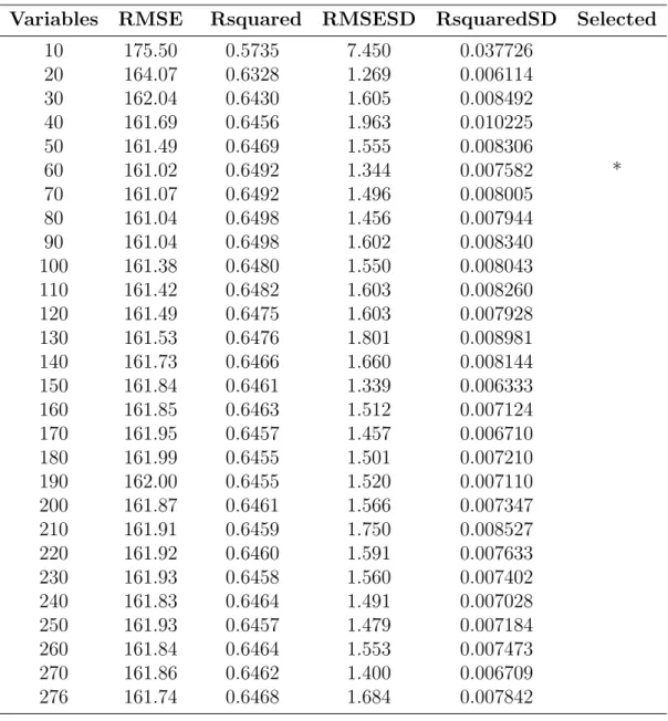
Table 4.1.: Results from the recursive feature elimination with random forest regression and resampling.
Variables RMSE Rsquared RMSESD RsquaredSD Selected 10 175.50 0.5735 7.450 0.037726 20 164.07 0.6328 1.269 0.006114 30 162.04 0.6430 1.605 0.008492 40 161.69 0.6456 1.963 0.010225 50 161.49 0.6469 1.555 0.008306 60 161.02 0.6492 1.344 0.007582 * 70 161.07 0.6492 1.496 0.008005 80 161.04 0.6498 1.456 0.007944 90 161.04 0.6498 1.602 0.008340 100 161.38 0.6480 1.550 0.008043 110 161.42 0.6482 1.603 0.008260 120 161.49 0.6475 1.603 0.007928 130 161.53 0.6476 1.801 0.008981 140 161.73 0.6466 1.660 0.008144 150 161.84 0.6461 1.339 0.006333 160 161.85 0.6463 1.512 0.007124 170 161.95 0.6457 1.457 0.006710 180 161.99 0.6455 1.501 0.007210 190 162.00 0.6455 1.520 0.007110 200 161.87 0.6461 1.566 0.007347 210 161.91 0.6459 1.750 0.008527 220 161.92 0.6460 1.591 0.007633 230 161.93 0.6458 1.560 0.007402 240 161.83 0.6464 1.491 0.007028 250 161.93 0.6457 1.479 0.007184 260 161.84 0.6464 1.553 0.007473 270 161.86 0.6462 1.400 0.006709 276 161.74 0.6468 1.684 0.007842
In Table 4.1. the result from the recursive feature elimination with random forest regression and resampling can be seen. Different subset sizes in steps of 10 were
4.2 Random forest regression
evaluated. The subset size with the minimum average RMSE is chosen as the best subset size. The subset size 60 has the minimum average RMSE and is selected as the best subset size. The performance metric R2 and the standard deviation of R2
and RMSE for the different subset sizes can also be seen in the table. From the table one can see that a subset size of 20 results in a significantly lower RMSE than a subset size of 10 does. There is no great difference in RMSE for the subset size of 20 and subset sizes greater than 20.
The best subset of variables out of the subset sizes tried contains 60 variables and among these variables the most important variable according to the variable im-portance measure in the random forest model is the variable corresponding to the difference between brightness temperature of the 11 and 12 micron channel. The texture of the temperature of the 11 micron channel as well as the brightness tem-perature of the 11, 12 and 3.7 micron channel were among the 5 most important variables for predicting cloud top pressure. The longitude and latitude and differ-ent temperature profiles were also among the selected variables from the recursive feature elimination with random forest regression and resampling.
4.2. Random forest regression
All the random forest models are trained on the 60 variables selected by the recursive feature elimination. Results from the parameter tuning and model performance on the test data is showed when using a random sample of 100 000 observations and all data and splitting the data into training, validation and test data. The best set of parameters obtained from the parameter tuning when using all data and splitting the data into training, validation and test data is also used in the models on the filtered data and data obtained by using stratified random sampling.
4.2.1. Results using simple random sampling
Table 4.2.: Results from the first grid search with 3-fold cross-validation.
Maximum depth Variables Trees Average validation MSE
50 10 500 16459.0 1000 16427.9 1500 16417.8 2000 16416.3 20 500 16923.0 1000 16886.1 1500 16880.4 2000 16871.4 30 500 17201.7 1000 17185.2 1500 17178.5 2000 17159.2 70 10 500 16469.8 1000 16422.2 1500 16413.8 2000 16417.4 20 500 16889.7 1000 16894.5 1500 16887.7 2000 16869.2 30 500 17180.1 1000 17179.3 1500 17173.1 2000 17168.7 None 10 500 16438.7 1000 16433.3 1500 16411.8 2000 16418.2 20 500 16925.2 1000 16883.8 1500 16877.1 2000 16872.5 30 500 17199.3 1000 17174.7 1500 17186.4 2000 17168.7
4.2 Random forest regression
In Table 4.2. the first grid search performed on a random sample of 80 000 is shown. All combinations of different values for the parameters maximum tree depth, number of trees and number of variables randomly selected at each split in the tree were tried using 3-fold cross-validation with MSE as the performance metric to evaluate the best set of parameters. The number of trees evaluated were: {500,1000,1500,2000}, the number of variables randomly selected at each split in the tree: {10,20,30} and the values for maximum tree depth: {50,70,None}. With no maximum tree depth is meant that the tree will grow until all leaves are pure or the number of observations in each leaf is one. From Table 4.2. it can be seen that the best model tried from the 3-fold cross-validation is a random forest model with 1500 trees, no maximum tree depth and 10 variables randomly selected at each split in the tree. This can be seen since this model results in the minimum average validation MSE.
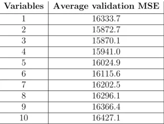
Table 4.3.: Results from the second grid search with 3-fold cross-validation.
Variables Average validation MSE
1 16333.7 2 15872.7 3 15870.1 4 15941.0 5 16024.9 6 16115.6 7 16202.5 8 16296.1 9 16366.4 10 16427.1
In Table 4.3. one can see the results from the second grid search where the number of trees is set to 1500 and the maximum depth of the tree is set to no maximum tree depth. For the different number of variables randomly selected at each split in the tree the numbers 1 to 10 were tried to see if a lower number of variables than 10 which was chosen in the first grid search would yield better results. The number of variables randomly selected at each split in the tree resulting in the minimum average validation MSE is 3.
Table 4.4.: Distribution of observations in the data obtained using a random sample of 100 000 observations. Training Test Low 20583 5094 Medium 12564 3274 High 46853 11632 All 80000 20000
Table 4.4. shows the distribution of observations across cloud classes for the training and test data when using a random sample of 100 000 observations. The same observations previously used for the 3-fold cross-validation is used as training data.
Table 4.5.: Cloud top pressure performance metrics for the random forest model trained on 80 000 observations.
RMSE MAE Bias bcRMSE Support Low 156.3 113.9 113.1 108.0 5094 Medium 84.7 61.6 26.6 80.4 3274 High 94.2 62.2 -56.7 75.2 11632 Overall 112.1 75.3 0.2 112.1 20000
In Table 4.5. the RMSE, MAE, the bias corrected RMSE and bias for the cloud top pressure can be seen for the model with the best set of parameters according to the second grid search performed on 80 000 observations. The random forest model with 1500 trees, 3 variables randomly selected at each split in the tree and no maximum tree depth has an overall RMSE of 112.1 hPA. The model was tested on 20 000 observations. The RMSE and MAE for low clouds are higher than for medium and high clouds. The signs of the biases indicate that low and medium clouds are more often estimated to have a lower cloud top pressure than the observed pressure while high clouds on the contrary are more often overestimated in terms of cloud top pressure.
Table 4.6.: Distribution of observations in the data obtained using simple random sampling.
Training Validation Test Low 73937 36884 37157 Medium 45162 22563 22216 High 168315 84260 84334 All 287414 143707 143707
Table 4.6. shows the distribution of observations across cloud classes for the training, validation and test data obtained using simple random sampling.
4.2 Random forest regression
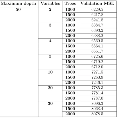
Table 4.7.: Results from the parameter tuning for random forest models with a maximum tree depth of 50.
Maximum depth Variables Trees Validation MSE
50 2 1000 6229.5 1500 6217.8 2000 6241.8 3 1000 6384.7 1500 6393.2 2000 6388.2 4 1000 6569.5 1500 6564.1 2000 6551.7 5 1000 6725.6 1500 6719.2 2000 6712.0 10 1000 7271.5 1500 7260.9 2000 7246.1 20 1000 7785.3 1500 7781.4 2000 7787.0 30 1000 8096.3 1500 8068.4 2000 8078.5
Table 4.7. shows the validation MSE for different number of trees and number of variables randomly chosen at each split in the tree for the maximum tree depth of 50. All data have been used and split into training, validating and test data. The number of trees evaluated are {1000,1500,2000} and the number of variables randomly selected at each split in the tree evaluated is {2,3,4,5,10,20,30}. In Table 4.7. it can be seen that a random forest model with a maximum tree depth of 50, 1500 trees and 2 variables randomly selected at each split in the tree results in the minimum validation MSE.
Table 4.8.: Results from the parameter tuning for random forest models with a maximum tree depth of 70.
Maximum depth Variables Trees Validation MSE
70 2 1000 6243.5 1500 6237.2 2000 6229.4 3 1000 6404.8 1500 6394.2 2000 6403.6 4 1000 6566.6 1500 6546.2 2000 6556.2 5 1000 6731.7 1500 6711.9 2000 6698.3 10 1000 7274.0 1500 7261.5 2000 7242.7 20 1000 7798.3 1500 7777.2 2000 7785.1 30 1000 8081.8 1500 8074.9 2000 8063.7
Table 4.8. shows the validation MSE for different number of trees and number of variables randomly chosen at each split in the tree for the maximum tree depth of 70. The number of trees evaluated are {1000,1500,2000} and the number of variables randomly selected at each split in the tree evaluated is {2,3,4,5,10,20,30}. In Table 4.8. it can be seen that a random forest model with a maximum tree depth of 70, 2000 trees and 2 variables randomly selected at each split in the tree results in the minimum validation MSE.
4.2 Random forest regression
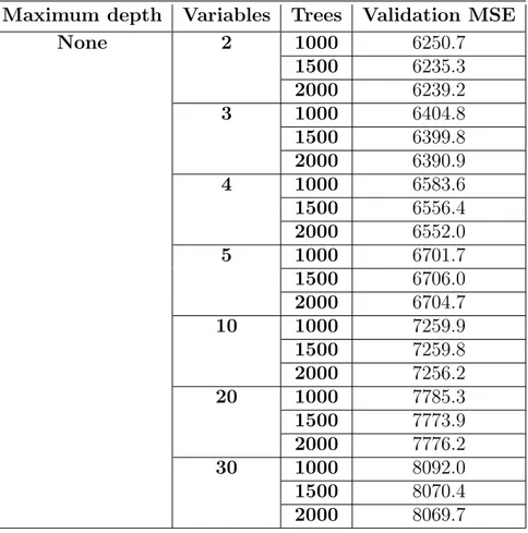
Table 4.9.: Results from the parameter tuning for random forest models with no maximum tree depth.
Maximum depth Variables Trees Validation MSE
None 2 1000 6250.7 1500 6235.3 2000 6239.2 3 1000 6404.8 1500 6399.8 2000 6390.9 4 1000 6583.6 1500 6556.4 2000 6552.0 5 1000 6701.7 1500 6706.0 2000 6704.7 10 1000 7259.9 1500 7259.8 2000 7256.2 20 1000 7785.3 1500 7773.9 2000 7776.2 30 1000 8092.0 1500 8070.4 2000 8069.7
Table 4.9. shows the validation MSE for different number of trees and number of variables randomly chosen at each split in the tree for no maximum tree depth, which is when the tree is grown until all leaves are pure or until all leaves contain one observation. The number of trees evaluated are {1000,1500,2000} and the number of variables randomly selected at each split in the tree evaluated is {2,3,4,5,10,20,30}. In the table it can be seen that a random forest model with no maximum tree depth, 1500 trees and 2 variables randomly selected at each split in the tree results in the minimum validation MSE.
The best set of parameters out of the parameters tried for the random forest model is a random forest model with 1500 trees, a maximum tree depth of 50 and 2 variables selected at random at each split in the tree.
Table 4.10.: Performance metrics for cloud top pressure for the random forest model trained on data obtained using simple random sampling.
RMSE MAE Bias bcRMSE Support Low 110.4 67.6 65.2 89.1 37157 Medium 63.2 40.8 11.1 62.2 22216 High 63.1 34.9 -30.5 55.2 84334 Overall 78.1 44.3 0.7 78.1 143707
In Table 4.10. the performance metrics for cloud top pressure for the random forest model with the best set of parameters according to the validation MSE are shown, which was 1500 trees, 2 variables chosen at random for each split in the tree and a maximum tree depth of 50. The random forest model has been trained on data obtained using simple random sampling. The overall RMSE is 78.1 hPA. Low clouds have a higher RMSE, MAE and bias corrected RMSE compared to medium and high clouds.
Figure 4.1.: Histogram of CALIPSO cloud top pressure.
Figure 4.1. shows a histogram of the observed cloud top pressure measured by the instrument on the satellite CALIPSO. The cloud top pressure has a bimodal distribution since mostly higher clouds with a low cloud top pressure is prevalent and the least prevalent cloud class is medium clouds.
4.2 Random forest regression
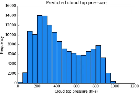
Figure 4.2.: Histogram of predicted cloud top pressure for the random forest model trained on data obtained using simple random sampling.
Figure 4.2. shows a histogram of the predicted cloud top pressure from the model with the best set of parameters obtained from the set of parameters tried on the validation data. The histogram shows that the predicted cloud top pressures also follows a bimodal distribution.
Table 4.11.: Performance metrics for interpolated cloud top height derived from the predicted cloud top pressures from the random forest model trained on data obtained using simple random sampling.
RMSE MAE Bias bcRMSE Support Low 1278.2 714.8 -688.2 1077.1 37157 Medium 916.4 561.6 -174.7 899.6 22216 High 1456.3 885.3 784.7 1226.8 84334 Overall 1340.5 791.2 255.5 1315.9 143707
In Table 4.11. the performance metrics for the interpolated cloud top height derived from the predicted cloud top pressures from the random forest model with the best set of parameters according to the validation MSE which was 1500 trees, 2 variables chosen at random for each split in the tree and a maximum tree depth of 50 are shown. The overall RMSE is 1340.5 m. When looking at the RMSE for the three different cloud classes one can see that the RMSE is highest for high clouds and lowest for medium clouds.
4.2.2. Results using stratified random sampling
Table 4.12.: Distribution of observations in the data obtained using stratified random sampling with more observations sampled from the low cloud class.
Training Validation Test Low 73989 36994 36995 Medium 44970 22485 22486 High 44970 22485 22486 All 163929 81964 81967
Table 4.12. shows the distribution of observations across cloud classes for the train-ing, validation and test data when using stratified random sampling where more observations belonging to the class low clouds are sampled.
Table 4.13.: Performance metrics for cloud top pressure for the random forest model. The model has been trained on data obtained using stratified random sampling with more observations sampled from the low cloud class.
RMSE MAE Bias bcRMSE Support Low 86.3 51.9 48.6 71.3 36995 Medium 59.3 38.2 -5.2 59.1 22486 High 131.6 91.2 -88.4 97.4 22486 Overall 95.3 58.9 -3.7 95.2 81967
In Table 4.13. the performance metrics for cloud top pressure for the random forest model with 1500 trees, 2 variables chosen at random for each split in the tree and a maximum tree depth of 50 are shown. The random forest model has been trained on data obtained using stratified random sampling with more observations sampled from the low cloud class. The overall RMSE is 95.3 hPA.
Table 4.14.: Performance metrics for interpolated cloud top height derived from the predicted cloud top pressures from the random forest model. The model has been trained on data obtained using stratified random sampling with more observations sampled from the low cloud class.
RMSE MAE Bias bcRMSE Support Low 943.6 527.8 -492.0 805.3 36995 Medium 810.9 510.3 56.2 808.9 22486 High 2882.8 2119.3 2054.5 2022.3 22486 Overall 1691.8 959.6 357.0 1653.7 81967
4.2 Random forest regression
In Table 4.14. the performance metrics for the interpolated cloud top height derived from the predicted cloud top pressures from the random forest model with the best set of parameters according to the validation MSE which was 1500 trees, 2 variables chosen at random for each split in the tree and a maximum tree depth of 50 are shown. The overall RMSE is 1691.8 m.
4.2.3. Results using simple random sampling on filtered data
Table 4.15.: Distribution of observations in the data obtained using simple random sampling on filtered data.
Training Validation Test Low 59116 29493 29332 Medium 33762 17105 16884 High 112279 55980 56363 All 205157 102578 102579
Table 4.15. shows the distribution of observations across cloud classes for the train-ing, validation and test data obtained using simple random sampling on filtered data.
Table 4.16.: Performance metrics for cloud top pressure for the random forest model trained on data obtained using simple random sampling on filtered data.
RMSE MAE Bias bcRMSE Support Low 90.8 56.0 54.2 72.9 29332 Medium 63.8 41.4 13.8 62.3 16884 High 70.8 38.0 -33.0 62.6 56363 Overall 76.0 43.7 -0.4 76.0 102579
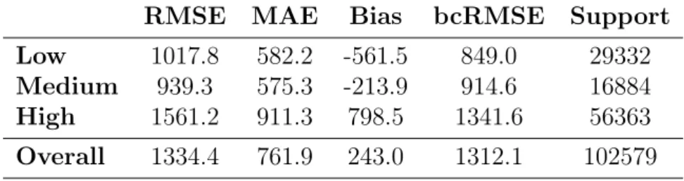
In Table 4.16. the performance metrics for cloud top pressure for the random forest model with 1500 trees, 2 variables chosen at random for each split in the tree and a maximum tree depth of 50 are shown. The random forest model has been trained on data obtained using simple random sampling on filtered data. The results show the performance of the random forest model on filtered data when observations with a total optical depth greater than 0.5 have been kept. The overall RMSE is 76.0 hPA.
Table 4.17.: Performance metrics for interpolated cloud top height derived from the predicted cloud top pressures from the random forest model trained on data obtained using simple random sampling on filtered data.
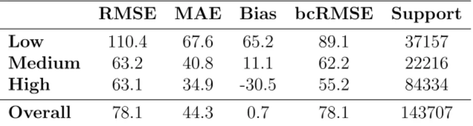
RMSE MAE Bias bcRMSE Support Low 1017.8 582.2 -561.5 849.0 29332 Medium 939.3 575.3 -213.9 914.6 16884 High 1561.2 911.3 798.5 1341.6 56363 Overall 1334.4 761.9 243.0 1312.1 102579
In Table 4.17. the performance metrics for the interpolated cloud top height derived from the predicted cloud top pressures from the random forest model with the best set of parameters according to the validation MSE which was 1500 trees, 2 variables chosen at random for each split in the tree and a maximum tree depth of 50 are shown. The model has been trained on filtered data where observations with a total optical depth greater than 0.5 have been kept. The overall RMSE is 1334.4 m.
4.2.4. Results using stratified random sampling on filtered data
Table 4.18.: Distribution of observations in the filtered data obtained using stratified random sampling with more observations sampled from the low cloud class.
Training Validation Test Low 58970 29485 29486 Medium 33875 16938 16938 High 33875 16938 16938 All 126720 63361 63362
Table 4.18. shows the distribution of observations across cloud classes for the train-ing, validation and test data obtained using stratified random sampling with more observations sampled from the class of low clouds on filtered data.
4.2 Random forest regression
Table 4.19.: Performance metrics for cloud top pressure for the random forest model. The model has been trained on data obtained using stratified random sampling on filtered data with more observations sampled from the low cloud class.
RMSE MAE Bias bcRMSE Support Low 69.0 41.9 39.0 56.9 29486 Medium 57.5 37.0 -1.8 57.4 16938 High 126.9 82.8 -78.8 99.4 16938 Overall 86.0 51.5 -3.4 86.0 63362
In Table 4.19. the performance metrics for cloud top pressure for the random forest model with 1500 trees, 2 variables chosen at random for each split in the tree and a maximum tree depth of 50 are shown. The results show the performance of the random forest model when observations with a total optical depth greater than 0.5 have been kept and stratified random sampling with more observations sampled from the low cloud class have been used. The performance metrics RMSE and MAE for both the low and medium clouds have improved now that the random forest model is trained on a larger proportion of low clouds compared to when not doing any stratified random sampling which led to the random forest model being trained on more high clouds since this is the most prevalent cloud class in the data.
Table 4.20.: Performance metrics for interpolated cloud top height derived from the predicted cloud top pressures from the random forest model. The model has been trained on data obtained using stratified random sampling on filtered data with more observations sampled from the low cloud class.
RMSE MAE Bias bcRMSE Support Low 733.6 422.1 -389.8 621.5 29486 Medium 798.2 498.0 9.6 798.2 16938 High 2642.7 1837.5 1746.1 1983.6 16938 Overall 1512.5 820.8 287.9 1484.9 63362
In Table 4.20. the performance metrics for the interpolated cloud top height derived from the predicted cloud top pressures from the random forest model with the best set of parameters according to the validation MSE which was 1500 trees, 2 variables chosen at random for each split in the tree and a maximum tree depth of 50 are shown. The model has been trained on filtered data where observations with a total optical depth greater than 0.5 have been kept. Stratified random sampling on filtered data with more observations sampled from the low cloud class have been used when training the model. The overall RMSE is 1512.5 m.
Table 4.21.: Distribution of observations in the filtered data obtained using stratified random sampling with an equal amount of observations sampled from each cloud class.
Training Validation Test Low 33875 16938 16938 Medium 33875 16938 16938 High 33875 16938 16938 All 101625 50814 50814
Table 4.21. shows the distribution of observations across cloud classes for the train-ing, validation and test data obtained using stratified random sampling with equal amount of observations sampled from each cloud class on filtered data.
Table 4.22.: Performance metrics for cloud top pressure for the random forest model. The model has been trained on data obtained using stratified random sampling on filtered data with an equal amount of observations sampled from each cloud class.
RMSE MAE Bias bcRMSE Support Low 92.4 62.3 60.7 69.7 16938 Medium 54.3 35.2 4.3 54.2 16938 High 115.9 75.3 -71.1 91.5 16938 Overall 91.2 57.6 -2.1 91.1 50814
In Table 4.22. the performance metrics for cloud top pressure for the random forest model with 1500 trees, 2 variables chosen at random for each split in the tree and a maximum tree depth of 50 are shown. The results show the performance of the random forest model when observations with a total optical depth greater than 0.5 have been kept and stratified random sampling with an equal amount of observations sampled from each cloud class have been used. The overall RMSE is 91.2 hPA. Compared to when a random sample with no regards to the three different cloud classes were taken the RMSE and MAE for the medium cloud class has decreased.
4.3 The multilayer perceptron
Table 4.23.: Performance metrics for interpolated cloud top height derived from the predicted cloud top pressures from the random forest model. The model has been trained on data obtained using stratified random sampling on filtered data with an equal amount of observations sampled from each cloud class.
RMSE MAE Bias bcRMSE Support Low 993.8 637.4 -619.4 777.2 16938 Medium 772.7 478.9 -67.5 769.7 16938 High 2476.4 1706.6 1608.8 1882.7 16938 Overall 1603.9 941.0 307.3 1574.2 50814
In Table 4.23. the performance metrics for the interpolated cloud top height derived from the predicted cloud top pressures from the random forest model with the best set of parameters according to the validation MSE which was 1500 trees, 2 variables chosen at random for each split in the tree and a maximum tree depth of 50 are shown. The model has been trained on filtered data where observations with a total optical depth greater than 0.5 have been kept. The model has been trained on data obtained using stratified random sampling on filtered data with an equal amount of observations sampled from each cloud class. The overall RMSE is 1603.9 m.
4.3. The multilayer perceptron
The number of variables used as inputs for the multilayer perceptron is 61. 60 of the variables are the ones chosen from the variable selection, where 57 variables are continuous and 3 variables are dummy variables representing 3 cloud type categories. When using weight decay in neural networks it is recommended to code categorical variables with 1-of-C encoding, meaning coding a variable with as many dummy variables as there are categories in a variable. This encoding is preferred since otherwise a bias toward output for the excluded category will be created [7]. A fourth dummy variable representing the category “other” is therefore created consisting of all the categories except the 3 categories that are represented by the chosen dummy variables from the variable selection. The dummy variable “other” together with the three other dummy variables for three different cloud type categories selected from the variable selection therefore creates a new variable representing cloud type. Parameter tuning when using a random sample of 80 000 oservations for the neural network is performed by using 3-fold cross-validation on 80 000 observations. The maximum number of epochs is set to 10 000. The performance metric used to evaluate the performance of the neural network models for each fold is the minimum validation MSE from the neural network training, the minimum average validation MSE from the three folds determines the model with the best set of parameters.
When using all data, filtered data and data obtained by stratified random sampling the parameter tuning is done by dividing the data into the 3 parts, training, valida-tion and test data. The maximum number of epochs used for all the data, filtered data and data obtained by using stratified random sampling is 20 000. The perfor-mace metric used to evaluate the best set of parameters is the minimum MSE for each run.
4.3.1. Results using simple random sampling
Table 4.24.: Average minimum validation MSE from 3-fold cross-validation.
Learning rate Hidden neurons 0.01 0.005 0.001 40 0.3210 0.3200 0.3163 60 0.3122 0.3086 0.3097 80 0.3111 0.3030 0.3085 100 0.3155 0.3013 0.3012 120 0.3157 0.3038 0.3007 140 0.3139 0.3044 0.2962 160 0.3143 0.3091 0.2971 180 0.3138 0.3038 0.2959 200 0.3171 0.3064 0.2994 220 0.3181 0.3040 0.2943 240 0.3150 0.3037 0.2967 260 0.3184 0.3047 0.2952 280 0.3185 0.3046 0.2950
Table 4.24. shows the average minimum validation MSE for the scaled data from the 3-fold cross-validation when using a momentum of 0.9 and a weight decay of 0.000001. The neural network model with minimum validation MSE is the model with a learning rate of 0.001 and 220 hidden neurons. For cross-validation a random sample of 80 000 observations was used.
4.3 The multilayer perceptron
Figure 4.3.: Average minimum validation MSE from 3-fold cross-validation.
Figure 4.3. shows the average minimum validation MSE for three different learning rates and different number of hidden neurons for the scaled data from the 3-fold cross-validation when using a momentum of 0.9 and a weight decay of 0.000001. In the plot one can clearly see that when using a learning rate of 0.01 the best model is with 80 hidden neurons and for a learning rate of 0.005 a model with 100 neurons is the best since it results in the lowest average minimum validation MSE. When having a higher number of neurons than 100 the lowest learning rate of 0.001 always results in the lowest average minimum validation MSE.
Table 4.25.: Results of change of the parameter momentum.
Momentum Validation MSE 0.7 0.2986 0.8 0.2969 0.9 0.2943
Table 4.25. shows the average minimum validation error for three different values for momentum for the scaled data from the 3-fold cross-validation when using a learning rate of 0.001, a weight decay of 0.000001 and 220 hidden neurons. The average minimum validation MSE for the three different values of momentum does not result in any big differences in MSE however a momentum of 0.9 has the lowest average minimum validation MSE.
Table 4.26.: Results of change of the parameter weight decay.
Weight decay Validation MSE 0.000001 0.2943
0.00001 0.3066
Table 4.26. shows the average minimum validation error for two different values of weight decay for the scaled data from the 3-fold cross-validation when using a learning rate of 0.001 and 220 hidden neurons. A higher value for weight decay, 0.00001 was tried but the lower weight decay of 0.000001 resulted in a lower average minimum validation MSE.
The best set of parameters for the neural network model with the lowest minimum average validation error from the 3-fold cross-validation is used to test its perfor-mance on the independent test data of 20 000 observations. When training the final model 60 000 observations of the 80 000 observations that have been used for cross-validation are used as training data and 20 000 observations are used as cross-validation data, that is monitored and used for deciding when the training of the network should stop. The best model chosen from the cross-validation has a learning rate of 0.001, a momentum of 0.9, a weight decay of 0.000001 and 220 hidden neurons. The weights from the epoch where the validation error is at a minimum is the model used for testing the predictive performance on the test data.
Table 4.27.: Distribution of observations in the data obtained using a random sample of 100 000 observations.
Training Validation Test Low 15482 5101 5094 Medium 9369 3195 3274 High 35149 11704 11632 All 60000 20000 20000
Table 4.27. shows the distribution of observations across cloud classes for the train-ing, validation and test data when using a random sample of 100 000 observations.
4.3 The multilayer perceptron
Table 4.28.: Performance metrics for cloud top pressure for the neural network model with 220 hidden neurons trained on data obtained using simple random sampling.
RMSE MAE Bias bcRMSE Support Low 176.1 128.0 101.1 144.1 5094 Medium 121.8 93.4 30.1 118.0 3274 High 130.4 91.7 -50.6 120.1 11632 Overall 142.2 101.2 1.3 142.1 20000
Table 4.28. shows the performance metrics for cloud top pressure for the test data and for the three different cloud classes represented in the data for the neural network trained on 60 000 observations. The overall RMSE is 142.2 hPA. The RMSE is lowest for medium clouds and highest for low clouds. The MAE is lowest for the high clouds. The negative value for the bias for high clouds indicates that the predicted values for cloud top pressure for high clouds is mostly higher than the observed cloud top pressure for these clouds. The low and medium clouds are mostly estimated to have a lower pressure than what is observed.
Table 4.29.: Distribution of observations in the data obtained using simple random sampling.
Training Validation Test Low 73937 36884 37157 Medium 45162 22563 22216 High 168315 84260 84334 All 287414 143707 143707
Table 4.29. shows the distribution of observations across cloud classes for the train-ing, validation and test data using simple random sampling when using all the data. Table 4.30.: Minimum validation MSE and training MSE for different number of hidden neurons for the neural networks. The models have been trained on data obtained using simple random sampling.
Hidden neurons Validation MSE Training MSE
200 0.2170 0.1959
300 0.2029 0.1771
400 0.1961 0.1686
In Table 4.30. the minimum validation MSE and training MSE at the same epoch for the scaled data is shown for the three neural network models with 200, 300 and
400 hidden neurons. The neural networks were trained using a learning rate of 0.001, a momentum of 0.9 and a weight decay of 0.000001. The model with 400 hidden neurons has the lowest minimum validation MSE of 0.1961. The training MSE is the average training MSE of all the batches of the training data.
Table 4.31.: Performance metrics for cloud top pressure for the neural network model with 400 hidden neurons trained on data obtained using simple random sampling.
RMSE MAE Bias bcRMSE Support Low 146.6 103.0 73.2 127.0 37157 Medium 104.5 79.2 16.7 103.2 22216 High 107.4 73.9 -38.7 100.2 84334 Overall 118.4 82.3 -1.2 118.4 143707
Table 4.31. shows the performance metrics for cloud top pressure for the neural network model with a log transformed response and 400 hidden neurons. The model has been trained on data obtained using simple random sampling. In the table it can be seen that the overall RMSE is 118.4 hPa. The cloud class medium has the lowest RMSE out of all cloud classes. From the bias in the table one can see that the low and medium clouds are mostly predicted to have a lower pressure compared to the observed pressure while the higher clouds are mostly predicted to have a higher pressure than what is actually observed.
Figure 4.4.: Observed and predicted cloud top pressure for the neural network with 400 hidden neurons trained on data obtained using simple random sampling.
4.3 The multilayer perceptron
Figure 4.4. shows boxplots of the predicted cloud top pressure for the neural network model with 400 hidden neurons as well as the observed cloud top pressure from the instrument on the satellite CALIPSO. The black line in the center of the boxplot represents the median. The line at the bottom and top of the box represents the first and third quartile. The black points outside the box represents outliers in the data.
A few outliers are present for the boxplot of the predicted cloud top pressure. Out of all observations 0.26% are predicted to have negative cloud top pressure which of course is outside the normal range of values for cloud top pressure.
The range of the predicted cloud top pressure is also a little wider than the range of the observed cloud top pressure from the more accurate instrument on the satellite CALIPSO.
4.3.2. Results using stratified random sampling
Table 4.32.: Distribution of observations in the data obtained using stratified random sampling with more observations sampled from the low cloud class.
Training Validation Test Low 73989 36994 36995 Medium 44970 22485 22486 High 44970 22485 22486 All 163929 81964 81967
Table 4.32. shows the distribution of observations across cloud classes for the train-ing, validation and test data obtained using stratified random sampling where more observations are sampled from the cloud class of low clouds.
Table 4.33.: Minimum validation MSE and training MSE for different number of hidden neurons for the neural networks. The models have been trained on data obtained using stratified random sampling with more observations sampled from the low cloud class.
Hidden neurons Validation MSE Training MSE
200 0.2311 0.1932
300 0.2233 0.1784
400 0.2222 0.1761
Table 4.33. shows the minimum validation MSE and training MSE for the same epoch for the scaled data for the neural network models with 200, 300 and 400
hidden neurons. The neural networks were trained using a learning rate of 0.001, a momentum of 0.9 and a weight decay of 0.000001. The model with 400 hidden neurons has the lowest validation MSE. The models were trained on data obtained using stratified random sampling with more observations sampled from the low cloud class.
Table 4.34.: Performance metrics for cloud top pressure for the neural network model with 400 hidden neurons. The model has been trained on data obtained using stratified random sampling with more observations sampled from the low cloud class.
RMSE MAE Bias bcRMSE Support Low 109.8 75.3 46.0 99.7 36995 Medium 94.1 70.1 -1.6 94.1 22486 High 158.1 112.1 -73.5 140.0 22486 Overall 121.3 84.0 0.2 121.3 81967
Table 4.34. shows the performance metrics for cloud top pressure for the neural network model with 400 hidden neurons. The model has been trained on data obtained using stratified random sampling with more observations sampled from the low cloud class. The overall RMSE is 121.3 hPA and the overall MAE is 84.0 hPA. The RMSE of low clouds has decreased a lot when training on more low clouds and instead the RMSE of high clouds has increased compared to when training on data obtained using simple random sampling. The cloud top pressure of low clouds is not as underestimated and the high clouds are more overestimated when training on more low clouds compared to when training on data obtained using simple random sampling. The medium clouds are mostly overestimated in terms of cloud top pressure.
4.3 The multilayer perceptron
Figure 4.5.: Observed and predicted cloud top pressure for the neural network model with 400 hidden neurons. The model has been trained on data obtained using stratified random sampling with more observations sampled from the low cloud class.
Figure 4.5. shows the observed and predicted cloud top pressure from the instrument on the satellite CALIPSO. A few observations are predicted to have a higher cloud top pressure than outside the normal range of values for cloud top pressure, one observation is particularly high and can be seen as an outlier in the boxplot for the predicted cloud top pressure. A few observations, 0.34% of the predicted values has negative values for cloud top pressure which is not within the normal range since pressure can’t be negative.
4.3.3. Results using simple random sampling with a log
transformed
When using the original response a few of the predicted values for cloud top pressure were negative due to the identity activation function at the output layer that can output values in the interval (-∞,∞). To restrict negative predicted values for cloud top pressure the response was log transformed. The exponentiated predicted values are then used for the calculation of the performance metrics.
Table 4.35.: Distribution of observations in the data obtained using simple random sampling.
Training Validation Test Low 73937 36884 37157 Medium 45162 22563 22216 High 168315 84260 84334 All 287414 143707 143707
Table 4.35. shows the distribution of observations across cloud classes for the train-ing, validation and test data obtained using simple random sampling.
Table 4.36.: Minimum validation MSE and training MSE for different number of hidden neurons for the neural networks with a log transformed response. The models have been trained on data obtained using simple random sampling.
Hidden neurons Validation MSE Training MSE
200 0.1877 0.1681
300 0.1749 0.1530
400 0.1709 0.1476
Table 4.36. shows the minimum validation MSE and training MSE for the same epoch for the scaled data when using a log transformed response variable. The neural networks were trained using a learning rate of 0.001, a momentum of 0.9 and a weight decay of 0.000001. The model with 400 hidden neurons has a lower minimum validation MSE than the models with 200 and 300 hidden neurons. Table 4.37.: Performance metrics for cloud top pressure for the neural network model with 400 hidden neurons and a log transformed response. The model has been trained on data obtained using simple random sampling.
RMSE MAE Bias bcRMSE Support Low 202.2 151.9 96.2 177.8 37157 Medium 127.6 92.8 30.0 124.0 22216 High 81.1 51.1 -27.8 76.1 84334 Overall 130.2 83.6 13.2 129.5 143707
Table 4.37. shows the performance metrics for cloud top pressure for the neural network model with a log transformed response and 400 hidden neurons. The model has been trained on data obtained using simple random sampling. The overall RMSE is 130.2 hPA and the overall MAE is 83.6 hPA. The low clouds have the highest
4.3 The multilayer perceptron
RMSE, MAE and bias corrected RMSE out of all three cloud classes. The low clouds are mostly predicted to have a lower cloud top pressure than observed and high clouds on the contrary are mostly overestimated and predicted to have a higher cloud top pressure than what is observed.
Figure 4.6.: Observed and predicted cloud top pressure for the neural network model with 400 hidden neurons and a log transformed response. The model has been trained on data obtained using simple random sampling.
Figure 4.6. shows two boxplots, one of the observed cloud top pressure from the instrument on the satellite CALIPSO and one of the predicted cloud top pressure from the neural network. A few of the predicted values have been predicted to have a higher cloud top pressure that is outside the normal range of values for cloud top pressure. One observation stands out and has been predicted to have an extremely high cloud top pressure.
Table 4.38.: Performance metrics for interpolated cloud top height derived from the predicted cloud top pressures from the neural network model with 400 hidden neurons and a log transformed response. The model has been trained on data obtained using simple random sampling.
RMSE MAE Bias bcRMSE Support Low 2391.8 1634.7 -1208.9 2063.8 37157 Medium 1857.9 1328.2 -546.5 1775.7 22216 High 1799.7 1249.4 635.2 1683.8 84334 Overall 1978.3 1361.2 -24.3 1978.1 143707