Propellers using Multi-Objective Genetic Algorithm
Aevan Nadjib Danial
Division of Fluid and Mechatronic SystemsMaster Thesis
Department of Management and Engineering
LIU-IEI-TEK-A–15/02411–SE
Propellers using Multi-Objective Genetic Algorithm
Master Thesis in Fluid Power
Department of Management and Engineering
Division of Fluid and Mechatronic Systems
Linköping University
by
Aevan Nadjib Danial
LIU-IEI-TEK-A–15/02411–SESupervisors: Patrick Berry
IEI, Linköping University Examiner: Christopher Jouannet
IEI, Linköping University Linköping, 29 November, 2015
Detta dokument hålls tillgängligt på Internet — eller dess framtida ersättare — under 25 år från publiceringsdatum under förutsättning att inga extraordinära omständigheter uppstår.
Tillgång till dokumentet innebär tillstånd för var och en att läsa, ladda ner, skriva ut enstaka kopior för enskilt bruk och att använda det oförändrat för icke-kommersiell forskning och för undervisning. Överföring av upphovsrätten vid en senare tidpunkt kan inte upphäva detta tillstånd. All annan användning av doku-mentet kräver upphovsmannens medgivande. För att garantera äktheten, säkerhe-ten och tillgänglighesäkerhe-ten finns det lösningar av teknisk och administrativ art.
Upphovsmannens ideella rätt innefattar rätt att bli nämnd som upphovsman i den omfattning som god sed kräver vid användning av dokumentet på ovan be-skrivna sätt samt skydd mot att dokumentet ändras eller presenteras i sådan form eller i sådant sammanhang som är kränkande för upphovsmannens litterära eller konstnärliga anseende eller egenart.
För ytterligare information om Linköping University Electronic Press se förla-gets hemsida http://www.ep.liu.se/
Copyright
The publishers will keep this document online on the Internet — or its possi-ble replacement — for a period of 25 years from the date of publication barring exceptional circumstances.
The online availability of the document implies a permanent permission for anyone to read, to download, to print out single copies for his/her own use and to use it unchanged for any non-commercial research and educational purpose. Subsequent transfers of copyright cannot revoke this permission. All other uses of the document are conditional on the consent of the copyright owner. The publisher has taken technical and administrative measures to assure authenticity, security and accessibility.
According to intellectual property law the author has the right to be mentioned when his/her work is accessed as described above and to be protected against infringement.
For additional information about the Linköping University Electronic Press and its procedures for publication and for assurance of document integrity, please refer to its www home page: http://www.ep.liu.se/
c
Abstract
This thesis showcases the challenges, downsides and advantages to building a Multi Disciplinary Optimization (MDO) framework to automate the generation of an effi-cient propeller design built for lightly loaded operation, more specifically for human powered aircrafts. Two years ago, a human powered aircraft project was initiated at Linköping University. With the help of several courses, various students per-formed conceptional design, calculated and finally manufactured a propeller by means of various materials and manufacturing techniques. The performance of the current propeller is utilized for benchmarking and comparing results obtained by the MDO process.
The developed MDO framework is constructed as a modeFRONITER project were several Computer Aided Engineering softwares (CAE) such as MATLAB, CATIA and XFOIL are connected to perform multiple consequent optimization subpro-cesses. The user is presented with several design constraints such as blade quan-tity, required input power, segment-wise airfoil thickness, desired lift coefficient etc. Also, 6 global search optimization algorithms are investigated to determine the one which generate most efficient result according to several set standards. The optimization process is thereafter initialized by identifying the most efficient chord distribution with a help of an initial blade cross-section which has been pre-viously used in other human powered propellers, the findings are thereafter used to determine the flow conditions at different propeller stations. Two different aero-dynamic optimized shapes are generated with the help of consecutively performed subprocesses. The optimized propeller requires 7.5 W less input power to generate nearly equivalent thrust as the original propeller with a total efficiency exceeding the 90 % mark (90.25 %). Moreover, the MDO framework include an automa-tion process to generate a CAD design of the optimized propeller. The generated CAD file illustrates a individual surface blade decrease of 12.5 % compared to the original design, the lightweight design and lower input power yield an overall propulsion system which is less tedious to operate.
Acknowledgments
This master thesis is the final project for a masters degree in Mechanical Engi-neering, Aeronautical engineering at Linköping University.
I would like to thank my supervisor Patrick Berry for giving me an opportunity to dive into such a complex investigation and for his support and brain-storming, Christopher Jouannet for his patience and guidance, Tomas Melin for taking his time to help me with his excellent parametric airfoil definition and XFOIL rec-ommendations and Raghu Chaitanya Munjulury for providing the essential airfoil CAD files. I could not have asked better people to support me through this long and tedious journey.
Also I’m extremely happy to have my close friends and classmates which I can share ideas and dig into psychophysical conversations with. Finally, I am proud to have such an amazing family which have given me the support, love and courage to complete this task.
Linköping, November, 2015 Aevan Nadjib Danial
Contents
1 Introduction 7
1.1 Background and Earlier Work . . . 7
1.1.1 Current Propeller Configuration . . . 8
1.2 Problem Area . . . 9
1.3 Objectives . . . 9
1.4 Delimitations . . . 10
2 Theory 11 2.1 BEMT Definition . . . 11
2.1.1 General Momentum Theory . . . 12
2.1.2 Blade Element Theory . . . 13
2.1.3 BEM Theory . . . 15
2.1.3.1 Interference Factors . . . 15
2.1.3.2 Tip Loss Correction Model . . . 16
2.1.3.3 Momentum Equations . . . 17
2.1.4 Propeller Design . . . 17
2.2 Parametric Airfoil Strategy . . . 19
2.2.1 Bézier Curve . . . 20
2.2.2 Geometry Parametrization . . . 21
2.3 XFOIL Analysis . . . 24
2.4 Optimization Algorithms . . . 25
2.4.1 Optimization Model Formulation . . . 25
2.4.2 Algorithms . . . 26
3 Methodology 29 3.1 XFOIL Strategy . . . 29
3.1.1 Panel Convergence . . . 30
3.2 BEM Theory Procedure . . . 32
3.3 Chord Optimization . . . 33
3.3.1 Current Chord Distribution Performance . . . 34
3.4 Airfoil Optimization . . . 36
3.4.1 Current Aerodynamic Performance . . . 37
3.5 CAD Subprocess . . . 38
3.6 Optimization: Initial Population Sampling . . . 39 ix
4.1 Results . . . 41
4.1.1 Optimization Algorithm Performance . . . 41
4.1.2 Chord Optimization . . . 44
4.1.3 Airfoil Optimization . . . 45
4.1.3.1 Airfoilst.1 . . . 45
4.1.3.2 Airfoilst.2,3 . . . 46
4.1.3.3 Airfoilst.4 . . . 48
4.1.4 Overall Performance Improvement . . . 49
4.1.5 Off-Design Aerodynamics . . . 50
4.1.6 Optimized CAD Design . . . 51
4.2 Discussion . . . 52
4.2.1 Proper Algorithm . . . 52
4.2.2 Airfoil Inverse Method . . . 53
4.2.3 Aerodynamic Data . . . 55
4.2.4 XFOIL Convergence . . . . 55
4.2.5 Computational Issues . . . 56
5 Future Work and Conclusions 57 5.1 Future Work . . . 57
5.2 Conclusions . . . 58
Bibliography 61
A ModeFRONTIER Project Trees 65
B Algorithm Convergence 71
C Design Data for Optimized Propeller 77
List of Figures
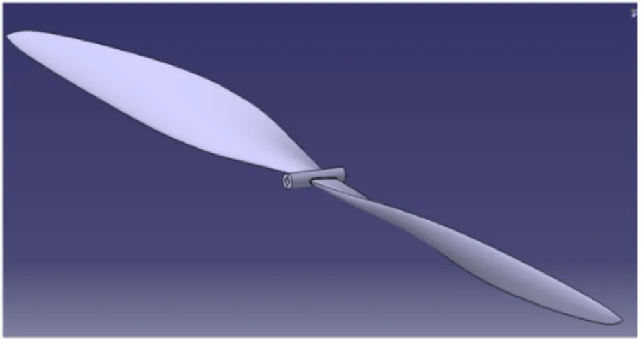
1.1 CAD illustration of the current propeller. . . 8 2.1 Momentum theory showing actuator disc in a controlled volume
with a pressure and velocity visualization. . . 13 2.2 flow diagram for blade element at an arbitrary radial location. . . 14 2.3 Force diagram on a blade element along with a view of propeller
geometry segmentation. . . 15 2.4 A visualization of the vortex flow generated by the propeller. . . . 16 2.5 Tip loss factor along the span of a propeller blade. . . 16 2.6 Bézier curve with control points P1− P3[1]. . . 20 2.7 Eppler 193 airfoil defined using the 13 control points definition,
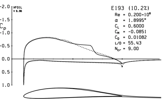
consisting of four individual Bézier curves (the airfoil is not to scale, to visualize control points strategy) [1]. . . 21 2.8 K1to K10 parameters for an Eppler 193 airfoil [1]. . . 22 2.9 K11to K14 parameters for an Eppler 193 airfoil [1]. . . 23 2.10 Example of an XFOIL output with Eppler 193 airfoil with specified
lift coefficient (CL= 0.6). . . . 25
3.1 General flow chart for XFOIL evaluation. . . . 30 3.2 Two script files sent to XFOIL for evaluations, different CL value
initialization and a range of CL values increase robustness of results. 30
3.3 Plots for CDand CM convergence for a range of panel quantity for
Eppler 193. . . 31 3.4 Plots for CDand CM convergence for a range of panel quantity for
DAE51. . . 31 3.5 General workflow for BEM theory. . . 33 3.6 Chord optimization flow chart. . . 34 3.7 various performance parameters for current propeller configuration
with Eppler 193 used as blade cross section. . . 35 3.8 Airfoil optimization flow chart for single or multiple stations. . . . 37 3.9 The shape of the four airfoils used for benchmarking. . . 37 3.10 workflow for CAD subprocess for an arbitrary propeller design. . . 38 3.11 Propeller blade with defined airfoils at 4 stations. . . 39 4.1 Optimization results for the 6 algorithms, MOGA-II shows most
promising result. . . 43 4.2 Design of the optimized airfoilst.1. . . 46
4.3 A comparison between the shape of the optimized airfoil for station 2 and 3 with the four benchmarking airfoils (Eppler 193 = red, DAE 51 = blue, Clark Y = green and Vortmann FX 60-100 = cyan). . . 47 4.4 The reused optimized shape of station 2 and 3. The trailing edge
thickness is very clear in this picture. . . 48 4.5 Local values for the optimized design along the non-dimensioned
4.6 Local Performance for the optimized design along the non-dimensioned propeller location ξ. . . . 50 4.7 CAD visualization of the optimized propeller with a simplified hub. 52 4.8 Curvature combs investigation for Airfoilst.1visualized with the help
of CATIA’s " Porcupine Curvature Analysis ". . . . 54 4.9 Curvature combs investigation for Airfoilst.2,3 visualized with the
help of CATIA’s " Porcupine Curvature Analysis ". . . . 55 A.1 ModeFRONTIER subprocess for BEM calculation. . . . 66 A.2 ModeFRONTIER main BEM calculation process with separate node
for best design extraction. . . 67 A.3 ModeFRONTIER subprocess for airfoil optimization. . . . 68 A.4 ModeFRONTIER main airfoil optimization process with external
node for best design extraction along with a final BEM calculation process. . . 69 B.1 Optimization convergence of MOGA-II. Airfoil thickness and drag
coefficients for station 2 and 3 for the feasible region are shown. Fast convergence is apparent. . . 72 B.2 Optimization convergence of NSGA-II. Airfoil thickness and drag
coefficients for station 2 and 3 for the feasible region are shown. More iterations are preferably required here, CD values are still
declining. . . 72 B.3 Optimization convergence of ARMOGA. Airfoil thickness and drag
coefficients for station 2 and 3 for the feasible region are shown. Slow convergence compared to MOGA-II. . . . 73 B.4 Optimization convergence of MOSA. Airfoil thickness and drag
coefficients for station 2 and 3 for the feasible region are shown. Slow convergence is apparent. . . 73 B.5 Optimization convergence of MOPSO. Airfoil thickness and drag
coefficients for station 2 and 3 for the feasible region are shown. This algorithm is not fitting for this optimization case. . . 74 B.6 Optimization convergence of ES. Airfoil thickness and drag
coef-ficients for station 2 and 3 for the feasible region are shown. Ex-tremely fast convergence similar to MOGA-II. . . . 74 B.7 Convergence of total efficiency η for chord optimization process with
MOGA-II algorithm. Propeller design with Eppler 193 as the ini-tialized cross-section seem to converge most efficiency. . . 75 B.8 Algorithm convergence for root station airfoil optimization using
MOGA-II. The plot to the right visualizes the drag minimization
in the feasible region. . . 76 C.1 Visualization of all airfoil shapes at each propeller station. . . 78 D.1 Aerodynamic performance of Airfoilst.1 for various free-stream
ve-locities at propeller station 1. decreased speed dramatically de-creases the performance as expected. . . 82
D.2 Aerodynamic performance of Airfoilst.2,3for various free-stream
ve-locities at propeller station 2. This airfoil is able to handle high list coefficients for even for very low velocities. . . 83 D.3 Aerodynamic performance of Airfoilst.2,3for various free-stream
ve-locities at propeller station 3. Airfoil performance is nearly unaf-fected by decrease in velocity. . . 84 D.4 Aerodynamic performance of Airfoilst.2,3for various free-stream
ve-locities at propeller station 4. Obtained results are nearly identical. Computational error occurs close to CDvalue of 0.1 where a sudden
decrease is obtained, low Reynolds number and inadequate panels distribution are the probable causes. . . 85
List of Tables
1.1 Current propeller configuration. . . 9
2.1 Control point definition for an arbitrary airfoil. . . 21
2.2 K-parameters range definition for design space minimization. . . . 24
3.1 Performance data for current propeller configuration with four dif-ferent airfoil section. . . 35
3.2 ε value for each blade station with four airfoil configurations for current blade design. . . 38
4.1 Maximum thickness for the tested airfoils. . . 42
4.2 Various optimization results from the 6 algorithms, MOGA-II ap-pears to be performing most efficiently. . . 42
4.3 Chord optimization for four different airfoil configurations, Eppler 193 seems to perform the best with highest efficiency difference ηdif f. . . 44
4.4 Results for the Optimized airfoil for station 1. . . 46
4.5 Aerodynamic efficiency comparison between the optimized shape with the four benchmarking airfoils specifically for propeller station 2. . . 47
4.6 Aerodynamic efficiency comparison between the optimized shape with the four benchmarking airfoils specifically for propeller station 3. . . 48
4.7 Performance check of the tip station. High CL values generates anticipated stall behavior. . . 49
4.8 Performance of the optimized propeller. . . 49
4.9 Reynolds numbers for decreased free-stream velocity V∞. . . 51
C.1 Design data for the optimized propeller. . . 78
C.2 station 1 . . . 79
C.3 station 2 . . . 79
C.4 station 3 . . . 79
Abbreviations
AoA Angle of Attack
BEMT Blade Element Momentum Theory
CATIA Computer Aided Threedimentional Interactive Application CAD Computer Aided Design
CAE Computer Aided Engineering CFD Computational Fluid Dynamics CPU Central Processing Unit CPT Computational Time FSI Fluid Structural Interaction HPA Human Powered Aircrafts MDO Multi Disciplinary Optimization
MOEA Multi-Objective Evolutionary Optimization MRF Multi Reference Frame
RAM Random Access Memory VLM Vortex Lattice Method QF Quantity of Feasible Designs
Nomenclature
a Axial Interference Factor
a0 Rotational Interference Factor
α Angle Of Attack
β Blade Twist Angle
c Chord Length
CL Lift Coefficient
CD Drag Coefficient
CT Thrust Coefficient
CP Power Coefficient
F Tip loss Correction Factor
φ Flow Angle
L/D Lift over drag coefficient
J Advance Ratio η Propeller Efficiency OP C Operating Conditions Ω Angular velocity Re Reynolds Number t/c Airfoil thickness V∞ Freestream Velocity Vc Speed of Sound
Chapter 1
Introduction
Optimization plays a huge role in today’s ever growing demand of reinventing in-dustrial applications or implementing further refinements and improvements on a particular component. To successfully manage this task, usually multiple software are used to subsequently improve and validate that the desired optimizations have been met.
This paper presents extensive work on the optimization process of a component that is used most commonly in aircrafts and wind turbines to produce thrust and extract energy from the air respectively, usually termed as propeller. With the help of a combination of chord, twist angle distribution and airfoil optimization one can design a propeller blade that is operating at its maximum efficiency at a given power requirement.
As earlier mentioned, multiple design utilities will be combined to develop a pro-peller blade that is specifically made for the endpoint of being the thrusting com-ponent of a human powered aircraft. This means that the propeller has to be designed with a specific power limited to what a human can produce. MATLAB,
XFOIL, modeFRONTIER are combined to form a framework for the design of
a propeller with optimized airfoil and chord distribution to maximize efficiency calculated using Blade Element Momentum Theory, BEMT [2].
1.1
Background and Earlier Work
Human powered aircraft (HPA) have been around for a very long time and the idea of being able to fly using power that is produced by the pilot is very fascinating and challenging on an engineering level.
This thesis work was initialized to maintain further development on the an on-going Human Powered aircraft project at Linköping University. Two different courses have been the base for the realization of this project including TMAL07
and TMAL08 [3] [4].
Specifically, The propulsion system being the propeller, of such an aircraft has been developed. Since it is being operated by a human, the design and configuration of the propulsion system will consequently define the structure and layout of the propeller blades to maximize operational efficiency at a given power input.
1.1.1
Current Propeller Configuration
JavaProp [5] is used as the main software for designing an efficient propeller for
the requirements set by various factor as cruise speed condition for lift off and ro-tational speed and propeller diameter. JavaProp uses pre-configured airfoil data, the current propeller is therefore defined by choosing the most appropriate air-foil at various stations along the span. The airair-foils used in the current propeller configuration is displayed in table 1.1 with an illustration of the CAD drawing in figure 1.1.
At the root chord, a thick airfoil (MH 126) was chosen since structural stability is favorable in that location thus being able to handle the produced torque. For the rest of the stations a much thinner airfoil best fitting for low Reynolds number operation is chosen (Eppler 193) since thrust is most prioritized in these locations. Table 1.1 also shows the airfoil twist at the various stations, these values were determined by manually twisting each airfoil to maximize L/D coefficient which consequently increases the total efficiency of the propeller. The airfoil at the root is only twisted slightly while the rest of the airfoils have a higher angle of attack to achieve maximum L/D coefficient where most of the thrust is produced. This behavior is clearly stated in JavaProp users guide that the thrust force is located 60 to 80 % of a propellers radius [6].
Table 1.1: Current propeller configuration.
specification value
Airfoil station 1 MH 126 Airfoil station 2,3,4 E 193 AoA (airfoil 1,2,3,4) 1◦,2◦,3◦,3◦
Chord length station 1-4 (m) 0.1, 0.1956, 0.1556, 0.0028
Nr of blades 2 Cruise speed 8.4 m/s Rotational speed 180 RPM Diameter 2.8 m Power input 260 W
1.2
Problem Area
As earlier mentioned, the current propeller design uses airfoils that are previously designed for certain applications. For example, the Eppler 193 airfoil which is in-tended for low Reynold operation was used as the airfoil section for the propeller design in the Human powered aircraft The Gossamer Albatross [7]. JavaProp
works in a similar manner, the user has the possibility to select between a few airfoils to create a optimum propeller for a certain power requirement.
Although this procedure is fail proof, it evidently means that the chosen airfoil section is not exclusively optimized for each station of the produced propeller. The aim is therefore to build a MDO framework that takes into account procedures that are included in available propeller optimization softwares. In addition to this, the framework will also include a sub optimization that creates airfoil section that are solely optimized for each station along the span of the propeller.
Furthermore, since this framework will sub optimize a propeller automatically, time consuming manual topological and morphological manipulations are elimi-nated resulting in relatively fast optimum propeller design.
1.3
Objectives
The objectives which have been targeted are listed below:
• Build a BEMT code in MATLAB that uses XFOIL to calculate drag coef-ficient for each blade station.
• Calculate the performance of the current propeller design to use the results as benchmark. I addition to this, utilize airfoils that have been used in earlier human powered propellers to calculate the performance of them also. • Investigate the most appropriate optimization algorithm.
• Perform spline interpolated chord optimization with modeFRONTIER at multiple stations with the addition of user constraints such as desired root and tip chords lengths.
• Subsequently perform airfoil optimization at each station to ensure that L/D is maximized while airfoil thickness and trailing edge gap constraints are met. • Output CAD drawing of the optimized propeller design.
• Combine the above mentioned process into a MDO framework with the appropriate user inputs.
1.4
Delimitations
The following points have been omitted:
• No validation process were included. No experimental data is available. • No user interface is included in optimization process, although sufficient
Chapter 2
Theory
Propeller optimization is usually carried out using multiple strategies. To minimize the optimization time of such a procedure, methods of low fidelity is usually cho-sen to give a fast indication of performance variation during variable manipulation. A rather simple propeller performance indicator, blade element momentum theory, is chosen as the core process. There are other methods such as VLM and high fidelity alternatives such as 3D CFD simulations, there methods were neglected since VLM is not as largely used as BEMT and the added computational time and power needed for CFD calculations are not justified for.
Airfoil geometry manipulations and analysis are explained to gain further under-standing about Bézier curves and XFOIL methodology. Furthermore, an overview of the available optimization algorithms is given to indicate their origin and help the prediction of the most appropriate technique.
2.1
BEMT Definition
Theories that explain the formulation of induced velocities in rotating components were initiated with the help of R. E. Froude [8] which introduced momentum theory followed by the actuator disc concept submitted by W. J. M. Rankine in late 19th century [9]. In addition to these theories, W. Froude contributed for the develop-ment of blade eledevelop-ment theory [10]. The increased developdevelop-ment of these theories were originally caused by the increase demand on more efficient ship propulsion system and helped diversify these conclusions into a wider range of applications. The fundamental operation of a marine propeller can be described as energy trans-fer and is therefore applicable to other applications such as wind turbines and non-marine propellers since they are only operating in a medium with different viscosity. H. Glauert [2] developed a theory which he termed as airscrew theory that is a combination of the earlier findings: blade element theory and momen-tum theory. (BEM) theory, despite its age, it is the most commonly used method
for calculating arbitrary propellers and wind turbines. This theory assumes that the propeller can be divided into finite number of strips, the flow conditions at each position can later be applied to the cross section (airfoil geometry) to calcu-late 2D aerodynamic forces. The total performance characteristics such as thrust and torque are obtained by summing or integrating the values for each annual position. Furthermore, the momentum theory is utilized to obtain the induced velocities that are resulting from the loss in momentum that affects the flow in the axial and tangential directions. These velocities alter the flow conditions at each annual section, the two methods are iterated until convergence in forces and flow parameters are reached.
2.1.1
General Momentum Theory
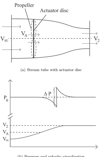
This fundamental theory was developed to understand axial motion of propellers passing through water with no understanding of the geometry of each propeller blade. Instead, it is replaced by a infinity thin and uniform actuator disc. This disc is positioned in a stream tube with two cross sections, inlet and outlet. A discontinuity in pressure at the location of the actuator disc occur since it is considered to absorb power (see figure 2.1(b)). Also, the velocity of the flow is increased in the aft section of the controlled tube since energy is added to the system. This analysis is applicable to wind turbines with the minor difference being the energy extraction and the flow velocity is therefore decreased behind such a system. The following assumptions are used for this theory:
• Compressibility effects, energy losses and unsteady flow are neglected • infinite number of blades
• Non-rotating wake • No friction drag
• The pressure at inlet and outlet of the control volume are equal to ambient static pressure
Figure 2.1(a) shows the stream tube with the actuator disc, V∞and V2are far up-stream and downup-stream from the actuator disc location. The velocity is increased along the length of the controlled volume and is reaching maximum value of V2. Using Bernoulli’s law and conservation of one dimensional momentum respectively, one can find the absorbed power and produced thrust are given by equations 2.1 and 2.2 where ˙m is the mass flow rate per time unit.
Pab= ( ˙ m 2)(V 2 2 − V∞2) (2.1) Tpr= ˙m(V2− V∞) (2.2)
(a) Stream tube with actuator disc
(b) Pressure and velocity visualization
Figure 2.1: Momentum theory showing actuator disc in a controlled volume with a pres-sure and velocity visualization.
2.1.2
Blade Element Theory
In this analysis, the propeller blade geometry is taken in consideration. As earlier mentioned, the blade geometry is divided into a large number of strips where the forces and flow parameters are calculated. Figure 2.2 shows a flow diagram of a airfoil cross section. a and a0, which are the axial and rotational interference factors respectively, are missing in blade element theory and will be explained later in 2.1.3.1. For now, the resultant velocity that is subjected to each blade element is comprised by V and Ωr which are the axial and rotational velocities respectively. It is very clear that the rotational velocity is variating with transition in radial location, which evidently contributed to change in flow characteristics for each subdivision.
Direction of rotation
Disc plane
Zero lift line
α φ β V (1 + a) Ωr(1− a′) W
Figure 2.2: flow diagram for blade element at an arbitrary radial location.
The angle φ is under normal operation condition smaller than the pitch angle β, this gives rise to an angle of attack α that contributes to the formation of lift and drag forces on each blade element. Using the simple definitions of lift and drag over an arbitrary airfoil cross section [11] and the contribution of φ, with simple trigonometry (see figure 2.3) one can calculate the thrust and torque contributions of each blade element [12] as shown in equations 2.3-2.6 where c is the chord length,
B is the number of blades. The number of divisions contribute large to the values
obtained and are usually between 20 and 50 subdivisions [6].
∆L = 1 2ρW 2cC L (2.3) ∆D = 1 2ρW 2cC D (2.4) T0 =1 2ρW 2BcC y (2.5) Q0 r = 1 2ρW 2BcC x (2.6) where
Cy= (CLcosφ − CDsinφ) = CL(cosφ − εsinφ) (2.7)
Cx= (CLsinφ + CDcosφ) = CL(sinφ + εcosφ) (2.8)
W. Froude may have failed to predict propeller performance accurately, he never-theless made a huge contribution to the later developed model (BEM) theory. His theory contained the basic idea with which the correct analysis could be formu-lated.
Direction of rotation
Disc plane
Zero lift line
α φ β L D T Resultant Q’/r r δr W
Figure 2.3: Force diagram on a blade element along with a view of propeller geometry segmentation.
2.1.3
BEM Theory
A half century later H. Glauert formulated a more accurate theory that describes propeller performance. Because of the simplicity of this model, some limitations emerge and are worth mentioning. One of these is the disregard of structural behavior of the propeller during operation, the blade tip tends to deflect away from its original state as a result of the added stress which in terms lead to a variation of aerodynamic inflow and force parameters. From momentum theory it is known that the momentum is balanced in a plane parallel to the disc plane which results in incorrect modeling. Furthermore, blade element momentum theory considers that the forces acting on a blade element are 2-dimensional which means that flow in the spanwise direction is neglected. highly loaded propellers experience large variation in pressure gradients along the span meaning that flow parameters for each blade element is essentially affected by the others. The above mentioned limitations lead to inaccurate calculations, however human powered propellers are in most cases lightly loaded meaning that these issues are less troubling.
2.1.3.1 Interference Factors
in subsection 2.1.2 it was mentioned that the formulation of induced velocities require correcting since it does not describe the real flow phenomena. The axial component was suggested to be equal to the freestream velocity V∞ but it is in reality increased slightly to account for the propellers own induced flow into the slipstream. Also, the rotational component should be less then the angular speed Ωr because of the vortex flow generated by the propeller (see figure 2.4). a and
a0, interference factors, are used to correctly formulate the axial and rotational velocities as shown in equations 2.9-2.10.
Vx= V∞(1 + a), Vθ= a0Ωr (2.9)
Vx
Vθ
X
V∞
Figure 2.4: A visualization of the vortex flow generated by the propeller.
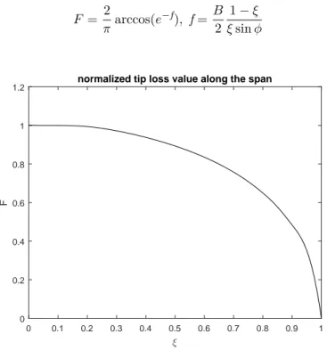
2.1.3.2 Tip Loss Correction Model
The pressure difference between the upper and lower surface of a propeller blade generates helical structures into the wake region, as shown in figure 2.4. These vortexes affect the induced velocity distribution at the propeller plane and most noticeably close to the tip of blades where most of the thrust is produced, it is therefore important to account for them. Prandtl developed a correction model that facilitates these structures to be of a rigid screw pattern [2]. Equation 2.11 shows the correction factor F where arccos(e−f) is in radians and ξ is the normal-ized radius. F = 2 πarccos(e −f), f = B 2 1 − ξ ξ sin φ (2.11) ξ 0 0.1 0.2 0.3 0.4 0.5 0.6 0.7 0.8 0.9 1 F 0 0.2 0.4 0.6 0.8 1
1.2 normalized tip loss value along the span
By observing figure 2.5 one can identify that the tip loss factor decreases as the radial location approaches the blade tip. This indicates that the relative wind speed decreases for each blade element which in terms affect the lift and drag forces produced. The assumption that the vortex created are of a rigid screw pattern limits its validity to lightly loaded propellers making this model sufficient enough for this application.
2.1.3.3 Momentum Equations
At this point, the momentum theory and blade element theory are used along with the tip loss correction model to calculate the thrust and torque produced by the propeller. The far stream velocity V2 need to be identified. It can be shown that the axial velocity at the disc is equal to the mean of the far upstream and downstream:
VA=
1
2(V2− V∞) (2.12)
Using equation 2.10 and the above equation, it is easy to find the far downstream axial velocity:
V2= 2(V∞(1 + a)) − V∞= V∞(1 + 2a) (2.13) The thrust produced can now be calculated. The mass flow rate ˙m = ρVAA is
calculated by identifying the area which is swept by the actuator disc A = 2πrδr as seen in figure 2.3. Using equation 2.2 the thrust can be identified as followed:
∆T = 2πrρV∞(1 + a)(V∞(1 + 2a) − V∞)F = 4πrρV∞2(1 + a)aF δr (2.14) Similarly to this, the angular momentum can be calculated by identifying the rotational velocity in the slipstream, which can be shown to be twice the value at the actuator disc plane:
Vθ2= 2Vθ= 2a0Ωr (2.15)
Again, conservation of momentum in the angular direction can be applied to find the torque produced (equation 2.16). The angular velocity Vθ1ahead of the
actu-ator disc plane is of course equal to zero since freestream one dimensional flow is assumed. ∆Q r = ˙m(Vθ2− Vθ1) = 2πrρV∞(1 + a)(2a 0Ωr)F = 4πr2ρV ∞(1 + a)a0ΩF (2.16)
2.1.4
Propeller Design
For a given propeller design with known chord distribution and airfoil cross section, the unknown variables described in the earlier text can be calculated. Initially the Reynold number is required to obtain inflow conditions at each blade segment and the following equation is therefore used [11]:
Re = ρW c
µ (2.17)
where
W =pV2
∞+ (Ωr)2 (2.18)
The obtained values are only initial estimates, however they do not vary greatly. Also, c is the chord distribution and µ is the dynamic viscosity in which the pro-peller is operating. since flow properties are known, the Reynold number can be used to find CD, ε and α for a given CL.
The loading equations 2.5 - 2.6 and 2.14 - 2.16 are required to be exactly equal and are therefore used to obtain a and a0 as seen below [12]:
a = σK (F − σK) (2.19) a0 = σK 0 (F + σK0) (2.20) where K = Cy 4 sin2φ (2.21) K0= Cx 4 cos φ sin φ (2.22)
and σ being the local solidity is:
σ = Bc
2πr
The flow angle φ is initialized at each blade segment using the following equation:
tan φ = 1
x (2.23)
where
x = Ωr V∞
The new flow angle can be found using figure 2.2 and equations 2.19 - 2.20: tan φ = [V∞(1 + a)]/[Ωr(1 − a0)] (2.24) The above equation is used as the new estimate for the flow angle and is substituted for the new φ until convergence have been reached. Finally, blade twist angle can be calculated using:
β = φ + α
At this stage, the thrust and power (P = 2πnQ) can be calculated followed by their respective coefficients as seen in equations 2.25 - 2.26 where n is the propeller rotation per seconds.
CT = T ρn2D4 (2.25) CP = P ρn3D5 (2.26)
To obtain the thrust and power coefficients for each blade element, the following equations are used [12]:
CT0 = (
π3
4 )σCyξF
32/[(F + σK0) cos φ]2 (2.27)
CP0 = CT0πξCx/Cy (2.28)
Finally the total propeller efficiency is:
η = CTJ CP
(2.29) where J = V∞/(nD) is the ratio of the advance distance to the propeller diameter.
2.2
Parametric Airfoil Strategy
The aerodynamic performance of a propeller is greatly dependent on the cross section geometry of each blade element. It is therefore very important to choose a cross section that can be operated at a certain criteria with the least amount of generated aerodynamic drag force. For many applications, such as airplane wing outer structure, a airfoil optimization process is performed to obtain a outer cross section shape which has good aerodynamic performance for a given design point. Several approaches to airfoil optimization can be found in many literatures. Be-cause of the popularity of airfoil optimization, a sub processor in the main MDO framework should be constructed to create airfoil shapes that are exclusively build for the aerodynamic flow characteristics of an adequate number of propeller blade stations.
airfoils such as Eppler 193 are defined using a large number of points (point cloud) and are accessible from airfoil databases such as UIUC Airfoil Coordinates
Database [13]. The coordinates consist of X and Y-components which are defined
as ratio of the normalized chord length. Optimizing a airfoil with point cloud will result in the formation of sharp edges as well as in the increase in required compu-tational power. To deal with this issue, different strategies can be used to minimize the design space such as defining airfoil geometry using spline or Bézier curves. T. Melin constructed an airfoil definition that employs Bézier curves defined with
13 control points [14] [1]. Bézier curves are widely used to create graphical mod-els with extremely smooth contours with a high degree of continuity and would therefore be most fitting for airfoil optimization and curvature definition.
2.2.1
Bézier Curve
The developed airfoil definition utilizes four Bézier curves which are manipulated using four control points, P0− P3. P0 and P1 are always defined as parallel to the Y-axis to obtain a leading edge which is tangential to it. Furthermore, P2and
P3 are instead parallel to the X-axis to give a smooth upper curvature. Figure 2.6 visualizes this along with the Bézier curve defined using Bernstein polynomial summation as seen in equation 2.30 [1].
P2 P3
P1
P0
Figure 2.6: Bézier curve with control points P1− P3 [1].
¯
B = (1 − t)3P¯0+ 3t(1 − t)2P¯1+ 3t3(1 − t) ¯P2+ t3P¯3 (2.30)
figure 2.7 shows the control point definition for Eppler 193 airfoil. It can be seen that the airfoil is constructed using four cubic Bézier curves which are connected at points 10 and 4 that control the upper and lower airfoil thickness respectively. Points 9, 10 and 11 have the same Y-coordinate which is also valid for points 3, 4 and 5. point 1 and 13 define the trailing edge thickness and their absolute value is therefore equal and their X-coordinate is equal to the normalized chord length. Finally, the X-coordinate for point 6, 7 and 8 will always be zero. This reduces the number of independent parameters to 14. Table 2.1 shows the control points coordinates for an arbitrary airfoil.
10 11 12 13 1 2 3 4 5 6 7 8 9
Figure 2.7: Eppler 193 airfoil defined using the 13 control points definition, consisting of four individual Bézier curves (the airfoil is not to scale, to visualize control points strategy) [1].
Table 2.1: Control point definition for an arbitrary airfoil. Coordinate Point X Y 1 1 -a 2 x2 y2 3 x3 b 4 x4 b 5 x5 b 6 0 y6 7 0 0 8 0 y8 9 x9 c 10 x10 c 11 x11 c 12 x12 y12 13 1 a
2.2.2
Geometry Parametrization
As earlier mentioned, the control points X and Y-value are defined as a ratio of the normalized chord length. A optimization process could be run on these values with a range from 0 to 1 but that create an unnecessary large design space. Instead, internal constraints are defined to prevent geometries that contain discontinuity in curvatures.
Points 10 and 4 which define the upper and lower airfoil thickness respectively are kept as they are. A maximum value of 15 % is set for those two points which can
be seen in equation 2.31. The maximum allowed airfoil "ram" thickness is therefore 30 %. The ram thickness will be slightly different from the final thickness t/c if the X-coordinates of point 4 and 10 are not equal (see figure 2.8).
y9,10,11= hu1= K5· 0.15
y3,4,5= hu2= K10· −0.15
(2.31)
The Y-coordinates for point 6 and 8 are defined using K1 and K6 as formulated below:
y8= K1hu1= K1K5· 0.15
y6= K6hu2= K6K10· −0.15
(2.32)
The X-coordinates for 10 and 4 are kept as parameters while 9, 11 and 3, 5 are dependent on them respectively as shown below:
x10= Pu1= K3 x4= Pu2= K8 x9= K2Pu1= K2K3 x11= K3+ K4(1 − Pu1) = K3+ K4(1 − K3) x5= K7Pu2= K7K8 x3= K8+ K9(1 − Pu2) = K8+ K9(1 − K8) (2.33) K7Pu2 (1 − Pu2) K2Pu1 K4(1 − Pu1) K9(1 − Pu2) (1 − Pu1) Pu1= K3 K1hu1 K6hu2 Pu2= K8 hu1 hu2
Figure 2.8: K1 to K10 parameters for an Eppler 193 airfoil [1].
One parameter which has been omitted is the trailing edge thickness, it is instead defined as a user input value T EG . The Y-coordinate for point 1 and 13 are defined as shown below:
y1= −T EG 2 c y13= T EG 2 c (2.34) Vmax1 K11Vmax1 K12Vmax2 Vmax2 β α Camber line
Figure 2.9: K11 to K14 parameters for an Eppler 193 airfoil [1].
The angle created between the camber line and the x-axis is defined as the release angle, α, which is a ratio of a maximum value of αmax= 20◦. Also, the Boat angle,
β, is defined as the angle between the tangents of the upper and lower side of the
airfoil and is set as a ratio of maximum value of βmax= 57◦ [1]. Observing figure
2.9 and the angle definitions, the X and Y-coordinates for 2 and 12 are defined as followed: x12= x11+ (K11Vmax1) = x11+ (K11(1 − x11)) x2= x3+ (K12Vmax2) = x3+ (K12(1 − x3)) (2.35) y12= tan(K14αmax+ K13βmax 2 )(1 − x12) + y13 y2= tan(K14αmax− K13βmax 2 )(1 − x2) + y1 (2.36)
The geometry parametrization is now defined using K1-K14 that have the range [0..1]. To minimize the design space even further, the upper and lower thickness positioning is ranging from [0.1..0.5] and upper and lower thickness have the range [0.1..1] since it is unnecessary to regard an airfoil thickness smaller than 3 % t/c (see table 2.2). The range defined here is general for any airfoil optimizations and will be utilized as the baseline parameters for individual propeller airfoil station optimization.
Table 2.2: K-parameters range definition for design space minimization. Parameter Range K1− K2, K4, K6− K7, K9, K11-K14 [0...1] K5, K10 [0.1...1] K3, K8 [0.1...0.5]
2.3
XFOIL Analysis
The aerodynamic calculation plays a huge role in the MDO framework since it is utilized in every sub-process. It is therefore very important to obtain fast and re-liable results while not requiring a huge amount of computational time and power. Navier-Stokes approaches can be used to predict airfoil flowfield (3D-flow) but it is too slow compared to interactive viscous/inviscid zonal approaches and does not yet acquire any accuracy advantages over it [15]. This is especially crucial when fast inverse airfoil design is needed.
Human powered propellers produce a very small amount of power which implies that airflow around airfoils on the propeller blade have low Reynolds number char-acteristics. The 2-dimensional coupled inviscid/viscous software XFOIL developed by MIT is chosen as the core aerodynamic analysis since it has been proven to output reliable airfoil flowfield prediction at reduced computational time.
The fundamental formulation of inviscid analysis in XFOIL is of a simple linear-vorticity streamfunction. Airfoil geometry and wake trajectory are discretized into a number of flat 2-dimensional panels with N nodes connected to the airfoil cur-vature. Kutta condition is used to calculate the surface vorticity of which surface pressure coefficient Cpcan be calculated from. XFOIL incorporate Karman-Tsien
compressibility correction which is not used in the scope of this paper since per-formance prediction of BEM theory is limited to incompressible flow conditions (below 0.35 Mach). The optimization framework will therefore include a check-point that dismiss any propeller design exceeding this condition. It can be noted that human powered aircraft usually operate at very low cruise speed condition and propeller rotation is limited, compressible flowfield condition is therefore a rare event.
Viscous formulation utilize a two-equation lagged integral to define the laminar and turbulent BL (boundary layer) with an envelope en transition criteria,
allow-ing proper calculation of limited separation region. velocity, wake, surface vorticity and viscous source distribution are calculated at each nodal point from the panel solution which is later solved using a Full-Newton method. The en transition is
always active and can be modified by the user-specified parameter "Ncrit". Stan-dard value of N crit = 9 (e9) which describe an average wind tunnel environment is used. Full description of XFOIL methodology can be viewed in [16].
Figure 2.10 shows a Cp over chord length plot of an Eppler 193 airfoil for a user
specified lift coefficient of 0.6 operating at a Reynolds number of 25. α, CM and
CD results are obtained within a few seconds.
Figure 2.10: Example of an XFOIL output with Eppler 193 airfoil with specified lift coefficient (CL= 0.6).
2.4
Optimization Algorithms
The necessary theoretical formulations for each sub processor are now defined, it is therefore logical to understand the importance of the optimization strategies. As earlier mentioned, the last essential software used is modeFRONTIER and it can be simply explained as a user interactive interface where various "Nodes" (integrated computer aided engineering (CAE) tools) such as MATLAB are coupled to form multi-objective and multi-disciplinary optimization platform. ModeFRONTIER offers a wide variety of optimization algorithms with deterministic, stochastic and heuristic methods.
2.4.1
Optimization Model Formulation
An optimization process can be represented mathematical formula that uses prob-lem choices as decision variables explore the design space to seek values that maxi-mize or minimaxi-mize the objective functions by applying constraints and limits to the variable parameters, it can be summarized by viewing the formulations below:
Subject to w(x) ≤ 0 z(x) = 0
f (x) is the matrix which contains the defined n number of objective function. x is
defined as the set of design variables that are subjected to inequality and equality constraints, w(x) and z(x) respectively. This formulation can be applied to single or multi-objective problems with the major difference that a single solution that is able to optimize all design objectives does not exist in a multi-objective problem. Instead, there exist a set of so called Pareto optimal solutions that non-dominantly optimize the objective functions.
2.4.2
Algorithms
optimization process can be divided into to segments: global search and local refinement. Global search facilitates an investigation of the whole design space to find the most optimum set of solutions (robustness) while local refinement is utilized for problems where the optimum region has been located (speed, accuracy).
ModeFRONTIER offers a wide variety of optimization algorithms that are capable
of handling such problems. The problems defined in this paper require increased robustness since aerodynamic flow, user constraints and structural considerations dictate the establishment of optimum airfoil cross section. With this in mind, the algorithms that are chosen belong in the category of heuristic optimizers to insure robustness in the output. The idea is to analyze the efficiency and speed of algorithms listed below to determine the most appropriate one with efficiency and time consumption kept in mind.
• MOGA-II Multi-objective Genetic Algorithm • NSGA-II Non-dominant Sorting Genetic Algorithm
• ARMOGA Adaptive Range Multi-objective Genetic Algorithm • MOSA Multi-objective Simulated Annealing
• MOPSO Multi-objective Particle Swarm Optimization • ES Evolutionary Strategy
Genetic algorithms mentioned above are optimization methods inspired by the improvement of species described by Darwinian theory [17]. First, a population of potential solutions are generated that undergo three basic optimization stages : selection, crossover and mutation. MOGA-II originated from the optimization algorithm MOGA and is an improved version with smart multi-search elitism. This prevents a premature convergence in a non-optimal local front to increase robustness [18].
NSGA-II is an improved version of the original NSGA non-dominant sorting
genetic algorithm [19] which have been criticized for lack of elitism, computa-tional complexity and the need for specifying a sharing parameter σshare. The
Pareto-optimal region [20].
ARMOGA is a fairly new developed algorithm that is based on MOEA
(multi-objective evolutionary algorithms) but introduces range adaption to adapt for optimization problems with restricted number of evaluations. statistical probabil-ity is used to adapt the search region from the already computed design points, the number of evaluations are therefore reduced to get a faster overview of the Pareto-optimal region [21] [22].
Evolutionary strategies ES is an optimization process that has the same funda-mental as the above mentioned algorithms where ideas of biological adaption and evolution are used to optimize a certain problem, it was initially developed by I. Rechenberg and H-P. Schewefel [23] [24]. Repeated steps are implemented where the initial population is variated slightly with crossover and mutation, offspring are generated from their parents. The offspring is evaluated by means of a "godness" level defined as fitness and the ones with better results are selected as parents for the next generation.
Simulated annealing SA received its name inspiration from annealing in metal-lurgy, a heat treatment technique where controlled heating and cooling of a mate-rial can alter its chemical properties to improve ductility. SA was first introduced in 1983 [25]. MOSA is a new approach that utilizes the algorithm from simulated annealing but can be used for multi-objective problems. This algorithm benefits from increased number of evaluation; the greater it is, the better robustness and convergence is achieved. Therefore it does not require as many initial population, also termed DOE (design of experiments), as MOGA-II [26].
Particle swarm optimization PSO was first developed by J. Kennedy and R. Eber-hart [27], the algorithm has its roots in artificial life such as bird flocking, fish schooling and more generally particle swarm theory. In PSO, a single solution is defined as a particle which "flys" over the problem design space and follow the optimum solution "guide". MOPSO is a modified version of the original algo-rithm, the definition of guide particle has been modified to facilitate the optimizer to converge into the region of optimal solutions. ModeFRONTIER utilizes the definition of MOPSO described in [28].
With a small introduction to each algorithm, it can be quite difficult to identify which of the algorithm that would satisfy the requirements of optimization prob-lems in this paper. It is evident that a robust and reliable method is required for airfoil optimization since propeller efficiency is greatly dependent on aerodynamic optimized blade cross sections. Also the fact that each XFOIL evaluation only requires seconds to run permits the use of global search methods with large num-ber of evaluations. By choosing these models, local refinement will be overlooked meaning that a "perfect" airfoil will not be produced. however, this procedure will guarantee a MDO framework that outputs optimized results independently on user inputs.
Chapter 3
Methodology
Building a multi disciplinary optimization framework pose a great deal of chal-lenges since it consists of multiple sub-processes that are linked to each other and failure rate increases as a result of that. It is therefore essential to construct each process carefully to eliminate insufficient or incorrect data transfer.
XFOIL analysis, BEM method, chord and airfoil optimization along with CAD
processes are described here. Preliminary results are presented here since they are necessary prior to final optimization results presented in chapter 4.
3.1
XFOIL Strategy
The automation process of airfoil analysis can be performed in various ways.
XFOIL can be initialized automatically with the help of batch files that contain
script files. The technique used in this paper is similar to the one in [29].
MATLAB is used to continuously update the script file to send the right airfoil
geometry data and flow characteristics for airfoil optimization and BEM theory calculations respectively. Airfoil geometry data for the BEM theory calculations is obtained from the parametric airfoil database of Tomas Melin while airfoil opti-mization obtain its airfoil file from the procedure described in section 2.2. Viscous simulations require Reynolds number input which is obtained from equation 2.17, it is different at each annual position along the propeller blade. Normally XFOIL evaluates a specified lift coefficient or angle of attack for 10 iterations, however this value is increased to 100 to allow solving for cases where dis-convergence is bound to happen, for example for high lift coefficients close to stall region. Finally, a sequence of CLis defined to assure that the airfoil design is useful for a wide range
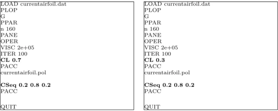
of CL. Figure 3.1 and 3.2 show the general flow chart for each XFOIL evaluation
along with two script files utilized for airfoil optimization respectively. 29
Load airfoil dat. file Define panel quantity (N) Viscous flow Re. number Define number of iterations Run sequence, CL1.... CLn or single value, CL save to file
Figure 3.1: General flow chart for XFOIL evaluation.
LOAD currentairfoil.dat PLOP G PPAR n 160 PANE OPER VISC 2e+05 ITER 100 CL 0.7 PACC currentairfoil.pol CSeq 0.2 0.8 0.2 PACC QUIT LOAD currentairfoil.dat PLOP G PPAR n 160 PANE OPER VISC 2e+05 ITER 100 CL 0.3 PACC currentairfoil.pol CSeq 0.2 0.8 0.2 PACC QUIT
Figure 3.2: Two script files sent to XFOIL for evaluations, different CLvalue initializa-tion and a range of CLvalues increase robustness of results.
3.1.1
Panel Convergence
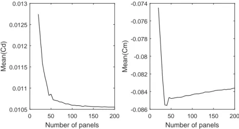
One important aspect of linear-vorticity panel method used in XFOIL is result convergence, the user is permitted to define the number of 2-dimensional panels that are projected into the airfoil geometry. Choosing a low quantity results in incomplete resolved pressure contours. Numerical accuracy is therefore tested for two airfoils (Eppler 193 and DAE 51) previously used in human powered propellers.
The flow characteristics for this analysis is taken from the original propeller design described in subsection 1.1.1 at the third radius location termed as blade station (between 60 to 80 % of propeller radius) where Reynolds number is approximate 2e5. Drag and moment coefficients are calculated from the same procedure shown in figure 3.2 for number of panels ranging from 10 to 200, the results are shown in figure 3.3 and 3.4. Number of panels 0 50 100 150 200 Mean(Cd) 0.0105 0.011 0.0115 0.012 0.0125 0.013 Number of panels 0 50 100 150 200 Mean(Cm) -0.086 -0.084 -0.082 -0.08 -0.078 -0.076 -0.074
Figure 3.3: Plots for CD and CM convergence for a range of panel quantity for Eppler 193. Number of panels 0 50 100 150 200 Mean(Cd) 0.011 0.012 0.013 0.014 0.015 0.016 0.017 0.018 Number of panels 0 50 100 150 200 Mean(Cm) -0.108 -0.1075 -0.107 -0.1065 -0.106 -0.1055 -0.105 -0.1045
Figure 3.4: Plots for CD and CM convergence for a range of panel quantity for DAE51.
it can be seen that convergence is reach when using approximately 140 panels or more. Panel quantity of 160 is therefore used for any future calculations, this value is chosen to insure that flow characteristics are resolved without any geometric dependency. This is even more important in the initial stage of airfoil optimization when large geometry fluctuations are observed.
3.2
BEM Theory Procedure
Considering the amount of user input variables that are included into an arbitrary propeller design, the BEM procedure requires most attention when designing a
MDO framework. It is used several times during the optimization process which
will be more evident in later sections.
The calculation process is initialized by defining various parameters. Free-stream velocity, dynamic viscosity, density of air, rotational speed and speed of sound are collectively termed as OP C. Chord at each station, number of blades (N b ), radius for blade and hub (Rblade and Rhub), desired constant lift coefficient (CL,des) and
Trailing edge thickness ( T EG) are also required by the user. Spline interpolation is utilized to form the total propeller shape along with other parameters such as the Mach number at each blade segment as see below.
mach = W Vc
(3.1) Subsequently, a design validations is performed to insure that certain requirements have been meet:
• Local maximum solidity is not exceeding unity
• local mach number is not exceeding 0.35 to prevent compressible flow • spline interpolations is not creating negative chord lengths at certain annual
position
Airfoil geometry and XFOIL evaluation is performed for each blade element to output angle of attack and CD
CL
= ε. There will be sent to the main calculation process that iterates the flow angle and the axial and radial interference factors (a and a0) until the new flow angle is within 2e−3 tolerance away from the old value. The iteration process is very fast and does not usually require more than 20 iterations to converge which only takes a few seconds.
Finally, the final blade twist distribution β is calculated along with the perfor-mance values; thrust, torque, power and efficiency. figure 3.5 shows an overview of the general flow-chart for performance calculation procedure.
Propeller blade design parameters chords1−4, N b, Rblade, Rhub,
OP C, CL,des, T EG
Initalize propeller design outputs : rrange,
chordsvect, Re, mach
Define airfoil geometry from database or parametric
XFOIL evaluations chordsvect, Re Check design σ < 1, mach < 0.35, spline interpolation if correct reject design if false Design calculations iterate φ, a, a′ αvect, εvect
Output propeller twist distribution and performance
β, T , Q/r, P , η
Figure 3.5: General workflow for BEM theory.
3.3
Chord Optimization
At already mentioned before, propeller calculation software usually define the blade by choosing airfoil geometry at 4 stations at different annual positions. This technique is therefore used to also define the chord distribution. The user is per-mitted to input the desired chord length for the root and tip chords which are kept as constants for two reasons; simplify future manufacturing process and maintain regard for structural stability at the root-chord where torque is transferred. The are two decision variables for this certain sub-process, the chord lengths for station 2 and 3. Spline interpolation maintains a smooth blade geometry granting that it passes through the design evaluation (explained in section 3.2) to reject unfeasible designs. Figure 3.6 shows the chord optimization procedure, the dotted
section is the core process that include the general BEM calculation along with the optimization algorithm. The maximum amount of power a human can developed is set to Pcontr= 260W , this value is used to limit the algorithm to approximately
optimize in that region with a ±1W tolerance. Also, a separate constraint is added to the decision variables (chords2− chords3> 0) to obtain the traditional blade design. The main objective for this optimization is the maximization of the total propeller efficiency at the defined power input, the excellence of each design evaluation is therefore used to generated new designs by manipulating the decision variables.
Decision variables chord2and chord3
Constraints N b, Rblade, Rhub, OP C, CL,des, T EG, Pcontr, chords1,4
Power constraint −1 < P − Pcontr< 1 DOE Algorithm BEM calculation
T , Q/r, P , η Objective
maximize η
Figure 3.6: Chord optimization flow chart.
Since there are various process levels to this optimization problem,
modeFRON-TIER facilitates the implementation of subprocesses that can be executed
inde-pendently of each other to minimize the decision making variables. The internal chord optimization scheduler (see figure A.1) is therefore built around the same principal as figure 3.6. To obtain a more user friendly experience, the MDO framework utilizes the internal subprocess to perform the requested optimization process for further analysis. At the point of completion, the complete design eval-uation sequence is sent to an external MATLAB node which locates the most excellent design that satisfies the defined power constraint region (see figure A.2)
3.3.1
Current Chord Distribution Performance
Prior to finalizing this subprocess, various airfoil configurations must be tested to determine the most appropriate for this task. The chord distribution is main-tained while changing the blade cross sections. Four airfoils are chosen, as seen below. These airfoils have been used in previous human powered propeller and are therefore good benchmarks for later results.
• Eppler 193, used in Gossamer Albatross propeller
• DAE 51, designed for low Reynolds numbers and used in Dadalus propeller • Clark Y, airfoil dated back to 1920 and have been used as propeller section • Wortmann FX 60-100, used as the propeller blade section on Velair Figure 3.7 shows the performance and current chord distribution. The most gen-erated power is located in the region already mentioned. By substituting Clark Y as the propeller blade cross section, a slightly higher total efficiency is observed as seen in table 3.1. It should be noted that the input power is exceeding the optimization limit set earlier which indicates that the current propeller is over-dimensioned. ξ 0 0.2 0.4 0.6 0.8 1 chord length [m] 0 0.05 0.1 0.15 0.2
local chord length
ξ 0 0.2 0.4 0.6 0.8 1 η 0 0.2 0.4 0.6 0.8 1 local efficiency ξ 0 0.1 0.2 0.3 0.4 0.5 0.6 0.7 0.8 0.9 1 Power [W] 0 5 10 15 20 25 Local power
Figure 3.7: various performance parameters for current propeller configuration with Ep-pler 193 used as blade cross section.
Table 3.1: Performance data for current propeller configuration with four different airfoil section. Airfoil Configuration Thrust T (N) Torque Q/r (N/m) Power P (W) Efficiency η (%) Power out Pout (W) Eppler 193 28.33 14.11 266 89.46 238 DAE 51 28.31 14.14 266.5 89.25 237.8 Clark Y 28.34 14.10 265.8 89.57 238.1 Vortmann FX 60-100 28.33 14.11 266 89.47 238
3.4
Airfoil Optimization
Aerodynamic performance is the highest contributer to total propeller efficiency and therefore requires most attention. Airfoil optimization can be performed in various ways, either by developing a optimized shape for each blade stations or by multi-objective optimization for various segments. The last mentioned method is in this case the most appropriate since propeller blades are formed by cross section interpolation, having various shapes would result in an uneven and structurally difficult design to manufacture.
Figure 3.8 shows the airfoil optimization process which is valid for single or mul-tiple objectives. There are 14 parameters that define the airfoil geometry, the values upper and lower levels are defined as in table 2.2 to minimize the size of the design space to a concentrated region of interest. The user is permitted to input the required airfoil thickness at each blade station ((t/c)contr), this value
is used to apply constraints to the airfoil geometry with the following relation: (hu1− hu2) − (t/c)contr ≥ 0. Also, an important constraint which controls the
relation between the upper and lower thickness heights: K5> K10is utilized. The first constraints insures that feasible deigns only belong to airfoil thickness that exceeds or is equal to the desired value. The second constraint steers the opti-mization algorithm to concentrate on the region where the upper thickness value is larger than the lower one to achieve the conventional airfoil shape.
A sequence of lift coefficients are tested to insure that the optimized airfoil shape is also performing optimally outside the defined constant lift coefficient CL,des. For
each XFOIL evaluation, two internal runs are performed following the guidelines as seen in figure 3.2 and the worst value is extracted to prevent initialization issues. An average value (CD,av) or multiple values ((CD,av,1)...(CD,av,n)) are thereafter
taken from each design evaluation. Minimization objective is applied to these out-puts and the process is repeated to generate new design generations with the help of the previous design excellence.
The principle used in the chord optimization is used here, Several subprocesses (see figure A.3) are successively executed. Station 1 is single-objective processes while station 2 and 3 are set as a single multi-objective optimization. However no process is applied for the propeller tip station because its aerodynamic efficiency does not influence the total performance of the propeller since tip loss correction model assumes zero local efficiency for the tip (see 2.1.3.2). An external MATLAB node is implemented to obtain the results from the executed processes and extract the most optimal design evaluations (see figure A.4). It can be seen that a final BEM calculation is included in the final process to obtain the performance and required design parameters for CAD construction.
Decision variables K1− K14
Constants CL,des, T EG, Revect, Chordsvect, (t/c)contr
constraints (hu1− hu2)− (t/c)contr≥ 0
K5> K10 CD,av< 1
DOE Algorithm XFOIL evaluation
CD,av Objective
minimize (CD,av,1)...(CD,av,n)
Figure 3.8: Airfoil optimization flow chart for single or multiple stations.
3.4.1
Current Aerodynamic Performance
The flow conditions is different at each blade station, each airfoil configuration would therefore perform differently. Figure 3.9 shows shape of the four chosen air-foils, they vary greatly since they were initially designed for a certain application. Most significant is the trailing edge shape of Vortmann FX 60-100.
0 0.2 0.4 0.6 0.8 1 -0.05 0 0.05 0.1 Eppler 193 0 0.2 0.4 0.6 0.8 1 -0.05 0 0.05 0.1 DAE 51 0 0.2 0.4 0.6 0.8 1 -0.05 0 0.05 0.1 Clark Y 0 0.2 0.4 0.6 0.8 1 -0.05 0 0.05 0.1 Vortmann FX 60-100

![Figure 2.7: Eppler 193 airfoil defined using the 13 control points definition, consisting of four individual Bézier curves (the airfoil is not to scale, to visualize control points strategy) [1].](https://thumb-eu.123doks.com/thumbv2/5dokorg/4622830.119326/33.701.131.585.105.289/definition-consisting-individual-bézier-airfoil-visualize-control-strategy.webp)
![Figure 2.8: K 1 to K 10 parameters for an Eppler 193 airfoil [1].](https://thumb-eu.123doks.com/thumbv2/5dokorg/4622830.119326/34.701.113.588.411.817/figure-k-k-parameters-eppler-airfoil.webp)