Marginal cost pricing of noise in railway infrastructure

(1)

Marginal Cost Pricing of Noise in Railway Infrastructure

∗

Henrik Andersson

Department of Transport Economics,

Swedish National Road & Transport Research Institute (VTI), Sweden

Mikael ¨

Ogren

Department of Environment and Traffic Analysis, VTI, Sweden

Abstract

In order to mitigate negative effects from traffic it has been decided that infrastructure charges in the European Union (EU) should be based on short run marginal costs. The Swedish Parliament has legislated that operators in the Swedish railway infrastructure must pay charges based on short run marginal social costs in order to mitigate externalities in railway infrastructure. Internalization of the social cost of noise is of particular interest, since it is the only environmental problem perceived as more troublesome today than in the early 1990s.

Inclusion of a noise component in rail infrastructure charges raises two issues: (i) the monetary evaluation of noise abatement, since noise is a non-market good, and (ii) the estimation of the effect on the noise level that one extra train will create. Regarding the latter, we are interested in the marginal noise, since infrastructure charges based on the short-run marginal cost principle should be based on the effect from the marginal train, not the noise level itself.

Using already existing knowledge, this study shows that it is possible to implement a noise component in the rail infrastructure charges. The values that are used today to estimate the social cost of noise exposure in cost benefit analysis can also be used to calculate the marginal cost. We recommend, however, that further research be carried out in order to get more robust estimates based on railway traffic. We also show that the existing noise estimation models can easily be modified to estimate the marginal noise. Noise infrastructure charges give the operators incentives to reduce their noise emissions. We believe that this kind of charge can be used to reduce overall emission levels to an optimal social level, but that it is important for the charge to be based on monetary estimates for rail-traffic and not road-traffic.

∗_{The authors would like to thank Mats Andersson, Karin Blidberg, Gunnar Lindberg, Rikard Nilsson, Ulf Sandberg, and Kjell Str¨ommer for}

valuable comments on earlier drafts of this chapter, and express their gratitude to Rune Karlsson for the constrained least squares polynomial fit of the marginal cost function. Financial support from Banverket is gratefully acknowledged. The authors are solely responsible for the results presented and views expressed in this chapter.

(2)

1 Introduction

Increased environmental consciousness among the general public has led to many of society’s environmental problems becoming stabilized or reduced through political influence and consumer power. Noise is one of the ex-ceptions, being the only environmental effect over which public dissatisfaction has increased since 1992 ( Öhrström et al., 2005). The transport sector is a major contributor to society’s increasing noise problem, due to increased traffic volumes and urbanization exposing more people to noise (Boverket, 2003; Nijland et al., 2003; Bluhm and Nordling, 2005; Kihlman, 2005a). Road traffic is admittedly the largest individual noise source in the transport sector, but other transport modes such as aircraft and railways are also responsible for considerable noise emis-sions (Kalivoda et al., 2003; Lundström et al., 2003). This chapter focuses on railway noise, a noise that largely differs from road traffic noise in that an essential part of the disturbance effect comes from individual noise peaks. Noise does not cause any direct environmental damage but entails costs for society in the form of disturbances for the individual (sleep, conversation, recreation, etc.), worsened health and lost productivity. A weakness, from an efficiency perspective, in the transport sector is that the whole noise cost is not borne by those who cause the noise, a so-called external effect. According to the Swedish Parliament’s transport policy decision of 1998 (Prop. 1997/98:56, 1998), operators using the state railways must pay a charge equivalent to the short run marginal social costs (SRMC) in order to mitigate the problem of externalities. Infrastructure charges based on SRMC internalize the external effects on the rest of the society and within the transport sector (e.g. congestion). Charges based on SRMC, thus, give operators incentives to contribute to a more efficient allocation of resources, and have the potential to result in an optimal traffic volume and use of technology.

Based on the Swedish legislation, Banverket (Swedish Rail Administration) and SIKA (Swedish Institute for Transport and Communications Analysis) were given a directive to propose a system of charges that would (SIKA, 2002a):

• better reflect the railway traffic’s short-run marginal costs on a practical level, at the same time as the operators are given plenty of signals about the desired adaptation of the activity and

• comply with EU legislation.1

The marginal costs for the transport sector on both national and EU levels are the short-run costs; that is, those that directly concern additional traffic.2 These are divided into five cost groups in the ”White Paper” (Rothengatter, 2003, p. 123); (i) operating costs, (ii) costs for the use and wear and tear of the infrastructure, (iii) crowding and scarcity costs, (iv) environmental costs and (v) accident costs.

1_{EU legislation requires pricing to be based on marginal cost principles, but permits “mark ups” as a means of financing infrastructure}

projects (European Commission, 1998).

2_{For the short-run marginal costs the infrastructure is assumed to be constant. A calculation of the long-run marginal costs also includes}

(4)

When reporting to the government, SIKA and Banverket came to somewhat different conclusions on noise and marginal costs (SIKA, 2002a). While SIKA was in favor of including marginal costs for noise in the system of railway infrastructure charges, Banverket’s contention was that noise costs should not be included. The latter was based on two standpoints. The first was that there was no basis for including noise costs since marginal cost calculations were lacking and that the average noise costs were not good indicators of marginal costs. The other reason was that charges would not be particularly effective means of influencing the noise from railway traffic.

Banverket has given VTI the task of investigating the prerequisites for pricing, with railway noise as one of the components in the charge to be paid by the railway operators. Thus, this chapter comprises three part-aims; (i) ascertain whether marginal noise for the railways exists and how it may be priced, (ii) analyse and make recommendations for how future noise evaluation studies should be formulated and what should be considered in them and (iii) make a sketch of how pricing, based on the estimation of marginal noise and noise value, may be designed.

This article is structured as follows. The next section is an outline of marginal cost pricing and externalities. Section 3 on noise first briefly discusses railway noise and thereafter how the marginal noise of trains may be estimated. Section 4 discusses different evaluation methods of noise exposure, followed by section 5 which goes through estimations of the pricing of railway noise. Finally the last two sections (6 and 7) proposes a structure for how a noise charge for railways may be constructed and contains the conclusions.

2 Marginal cost pricing

This section provides an outline of the economic argument for why railway infrastructure charges should be based on marginal cost pricing. We will not discuss the conflict between the marginal social cost principle, and long-run incremental costs and full cost recovery. Instead we refer to other literature for discussions on charging principles or financing problems, e.g. Nash (2005), Rothengatter (2003), or Sansom et al. (2001).

2.1 Externalities and economic efficiency

An allocation is socio-economically optimal when the value of the last produced unit is equal to its marginal cost. If the value is higher than the marginal cost, more resources should be allocated to the production of the good at the cost of alternative production. If the value is lower than the marginal cost, the resources should be reallocated to other production alternatives. This relationship is illustrated in Figure 1. The marginal cost function is represented by MCpand the demand function by D. The optimal consumption level is at the point of intersection of MCpand

D, that is, at quantity Qp.

The optimal quantity Qpis the result of the direct marginal cost. However, consumption often gives rise to

(5)

This negative externality may be termed an indirect cost and thus society’s social marginal cost consists of the sum of the direct and indirect marginal costs. The social marginal cost is given in Figure 1 by MCeand optimal

consumption then is Q∗_e. The welfare loss of consuming the quantity Qpinstead of Q∗eis shown by b, since the

values of the last units produced are lower than their marginal costs.

-6 !!!! !!!! !!!! !!!! !! !!!! !!!! !!!! !!!! !! PPP PPP PPP PPP PPP_PP P MCe MCp Q τ D P a b c c Q_τ Q∗_e Qp

Figure 1: Marginal cost pricing and economic efficiency

Assume now that price and quantity are not determined by the similarity between D and MCpor MCe, but that

there is a fixed charge equal toτ. Sinceτis higher than the price that would otherwise prevail, a lower quantity will be demanded, Q_τ. The welfare loss of this too high charge, compared to the case where equilibrium is given by MCp= D, is denoted by the areas a and c in Figure 1. The welfare loss is not as large when equilibrium is

determined by the social marginal cost MCe, in which case the welfare loss is denoted by a.3

3 Railway noise and marginal noise

The noise levels that people are subjected to normally originate from more than one source. ¨Ohrstr¨om et al. (2005) investigated the level of disturbance when the noise came from both road and railway sources and found that people were more disturbed by a combined sound than two separate ones, and that their respondents were more disturbed by railway noise than road noise, which runs counter to what other have found.4

Bluhm and Nordling (2005) found a clear connection between exposure and the level of disturbance. They also found that sleep disturbance, both the falling asleep problem and disturbed night sleep, increased with exposure. Another interesting result of Bluhm and Nordling (2005) was that the disturbance level of railway noise was more correlated with the equivalent level than with the maximum level. The maximum level is the most commonly used

3_{See e.g. S¨oderstr¨om (2002) (in Swedish) for a discussion on the ¨}_{Oresund Bridge and the difference between the current bridge toll and the}

marginal cost of a crossing.

4_{The authors suspected that the respondents’ answers to questions on railway noise may have been influenced by the plans for two more}

(6)

indicator in regulations against sleep disturbance.

3.1 Noise from railway traffic

The main source of railway noise is what is known as the rolling noise. Unevenness of the wheels and rails creates vibrations that are then emitted as sound. For low frequencies the rails are the principal noise source, while high frequencies are dominated by wheel sounds. Other sources that contribute are aerodynamic sound at high speeds, noise from fans in the engine and carriages, curve squeal and sounds from braking (see Hartung, 2000). A special problem is the unevenness caused by the brake pads of mainly freight trains, which leads to higher noise levels even when the brakes are not being used (Petersson, 1999). UIC (International Union of Railways) has taken an initiative in this area and shown that an improvement of about 8-10 dBA is attainable if the brake-pad system is replaced using state of the art technology (UIC, 2005).

There have been joint Nordic noise estimation methods for railway traffic dating back to 1984. The current method, called NMT96 (Naturv˚ardsverket, 1996), has been in use since 1996. The basis of the method is source parameters, combined with the speed, that describe the noise effect per meter for a given train type. The total train length that passes a given point gives the equivalent level, and the maximum level is determined by the maximum train length for the noisiest train type. Moreover, the method takes into account distance from the track, whether the ground is soft or hard, whether there is screening and several other parameters. A prerequisite for the usability of the method is that new source data is published when new train types are introduced.

New and improved methods have been developed since 1996. The so-called Nord 2000 (Plovsing and Kragh, 2000a,b) method has been developed in the Nordic countries and work on new joint methods has been ongoing in the EU with the projects HARMONOISE and IMAGINE (de Vos et al., 2005; Imagine, 2005) for all types of community noise. The largest changes compared to the previous generation of methods concern the accuracy for long distances, effect of the weather and screening. When these methods become operative, they will constitute a solid foundation for all types of community noise calculations in the EU.

3.2 Two examples of marginal noise calculation

Marginal noise is the increase of the sound level caused by an extra train set along a given stretch. This change can then be used to calculate the marginal cost of this train type if the relation between the sound level and the corresponding cost is known.

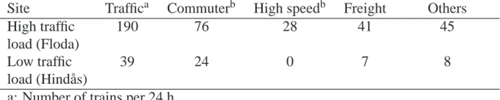
Two Swedish examples are given here to illustrate how marginal noise can be calculated, one with a high traffic load (Floda, western mainline) and one with a low load (Hind˚as, Bor˚as line). In a 24-hour period 190 and 39 trains pass through Floda and Hind˚as, respectively. Traffic data is summarized in Table 1.

(7)

Table 1: Rail traffic at example areas.

Site Traffica Commuterb High speedb Freight Others

High traffic 190 76 28 41 45

load (Floda)

Low traffic 39 24 0 7 8

load (Hind˚as)

a: Number of trains per 24 h.

b: The Swedish notations for the commuter and high speed trains are X14 and X2.

notation X14), a high speed train (X2) and a freight train, see Table 2. In both cases the traffic is somewhat simplified and the land around the track at the time of estimation is assumed to be flat and acoustically hard. Hence, the sound levels are overestimated somewhat compared to places with soft ground. It is also important to include the effects of noise screens wherever they exist. The total level is affected by both screens and soft ground, while noise changes are affected to a much lower extent. This means, in principle, that there is no obstacle to including both the screening and ground effects in the estimations. Indeed, both are included in NMT96 and the future models HARMONOISE/IMAGINE.

Table 2: Train sets used for estimating the marginal cost. Speed [km/h]

Train Length [m] Floda Hind˚as

Commuter (X14) 50 120 100

High speed (X2) 200 135 100

Freight 650 100 100

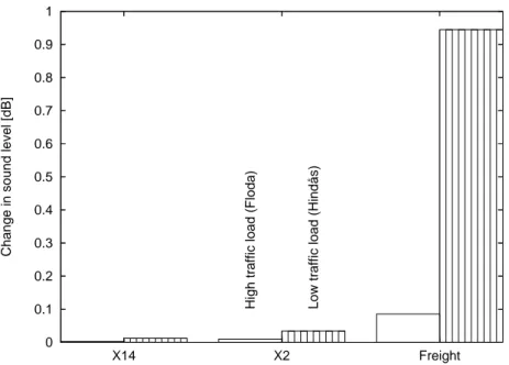
Figure 2 shows the estimated increase of the equivalent A-weighted sound level for a 24-hour period (LA,Eq,24h).5

The largest increase (0.9 dBA) is for freight trains and the increases are larger at the low-traffic site since fewer trains contribute to the total level. The lowest effect is for passenger trains in the high-traffic site, 0.003 dBA.

It is relatively easy to estimate the change in equivalent level for a train set, but estimating the effect on the maximum level is a more difficult matter. According to the methods available, the noisiest among all the train sets in traffic on the investigated line determines the maximum level. Hence, only one train set affects the maximum level, often the longest freight train in traffic, while the rest do not contribute to the maximum level at all. In other words, the maximum level is independent of the traffic volume in the estimation model, and the change in the maximum level is zero for all trains except the noisiest. In reality the probability that an extra noisy train will pass if the traffic is high is increased. It may also be that the maximum level is determined by different train types on different days depending on random factors such as wheel wear, number of freight wagons and so on.

The maximum level is used mainly as an indicator of sleep disturbances. Another indicator that is becoming increasingly more important in the EU is Lden, “level day, evening night”. This is an equivalent level (that is, all

(8)

trains contribute) but traffic in the evening and at night is punished with 5 and 10 dB penalty according to the formula (European Commission, 2000a):

Lden= 10 log µ 12 2410 0.1 Ld+ 4 2410 0.1 (Le+5)₊ 8 2410 0.1 (Ln+10) ¶ , (1)

where Ld, Leand Lndenote the equivalent noise levels for the day, evening and night period, respectively. The

intention is to create a unit value for noise disturbance that will represent both general disturbance, which is described as the equivalent level, and sleep disturbance, which is described as the maximum level at night. L_den is the noise indicator that will apply in the EU in future. In the example above goods traffic will dominate even more if we calculate Ldeninstead of LA,Eq,24h. Since Ldenis only a recalculation of the equivalent levels for three

periods, it is easy to adapt NMT96 to it if the traffic distribution over a 24-hour period is known.

0 0.1 0.2 0.3 0.4 0.5 0.6 0.7 0.8 0.9 1 Freight X2 X14

Change in sound level [dB]

High traffic load (Floda) Low traffic load (Hindås)

Figure 2: Change in A-weighted equivalent sound pressure level due to one extra train passage per 24 h, empty bar is for high traffic load (Floda) and filled bar for low traffic load (Hind˚as).

4 Preference elicitation

4.1 Evaluation of noise

As noise itself is a non-market good, there are no direct observable market prices for the value of reducing noise levels. For so-called non-market goods, apart from noise, e.g., safety and clean air, methods have therefore been developed to estimate individuals’ preferences. These methods are usually divided into two main groups depend-ing on what information is used. Preference estimations based on market data are called “revealed preferences” (RP) because they are based on observed behavior. The alternative is to estimate so-called “stated preferences”

(9)

(SP) in which it is clear that individuals have given their preferences in hypothetical market situations, e.g. answers to questionnaires and interview questions.

An overwhelming majority of noise evaluation studies use the RP approach and the method employed is the hedonic regression technique (Navrud, 2004). The hedonic method was formalized by Sherwin Rosen (1974) and has its point of departure in the fact that the prices of goods depend on their utility-bearing attributes. By studying how house prices are affected by exposure to noise, at the same time as effects on the price of other attributes are controlled for, it is possible to estimate the marginal willingness to pay (WTP) to reduce the noise level. The “noise sensitivity depreciation index” (NSDI), which is a measure of the percentage change in price resulting from a unit change in noise level, is used to compare the results of different hedonic price studies of noise evaluation.6 Bateman et al. (2001) reviewed the estimated NSDI values of various studies. The values varied from 0.08 to 2.22 with a mean of 0.55. The mean value implies that a dBA increase would reduce property values by just over half a percent.

One of the strengths of hedonic price studies is that they are based on individuals’ actual behavior and thereby their actual WTP.7A drawback, though, is that it can be difficult if not impossible to estimate the values that are of interest. SP methods, since they enable the analyst to tailor the survey/experiment, make it possible to elicit individuals’ preferences for specific noise circumstances. For instance, using a sample of residents near Bromma airport outside Stockholm, Carlsson et al. (2004) carried out an SP study in the form of “choice experiments” with the aim of estimating individuals’ preferences for aircraft noise at different times of the day and on weekdays and holidays. The results indicate a higher WTP to reduce noise level on weekday evenings and weekends, holidays and working days alike.

The SP method that is used most extensively for evaluating noise is the “contingent valuation method” (CVM) (Navrud, 2004). There are several different ways of designing CVM studies, but common for all of them is that the respondents directly state their WTP for the good (Bateman et al., 2002), here a reduction of the noise level. The advantage of the CVM and other SP methods is, as mentioned above, that the person conducting the study is allowed to construct it and can thus ask the questions he/she wants answers to and control for how different factors, e.g., study design, may have affected the results. The drawback is that the answers are to hypothetical questions and that there is no guarantee that the respondents will actually act as they have answered. This is a generally known phenomenon and several factors may explain why people answer like they do. One that is often

6_{Let P(A) and dBA denote the house price as a function of the attribute vector A and the noise level (which is included in A); then NSDI is}

given by (Bateman et al., 2001): NSDI =

¯ ¯ ¯

¯change in P(A) due to noise exposure_{change in dBA}

¯ ¯ ¯ ¯ ×_P(A)100 = ¯ ¯ ¯

¯% change in P(A)_{change in dBA}

¯ ¯ ¯ ¯ .

7_{For example, the price of a house is affected not only by exposure to noise but also by the number of rooms, view and so on. The hedonic}

(10)

mentioned is “hypothetical bias”, which refers to an overestimation of the WTP since the respondent is aware that he/she does not really have to pay the amount in question. Other problems frequently linked to CVM studies are insensitivity to the quantity of the good, strategic answers, and poorly constructed studies (see e.g. Kahneman and Knetsch, 1992; Carson et al., 2001; Bateman et al., 2002).8

The official Swedish monetary values that are currently in use as a basis for the estimation of noise costs for both roads and railways (SIKA, 2002b) rest heavily on the results from a hedonic pricing study which investigated how road noise affected house prices in ¨Angby outside Stockholm (Wilhelmsson, 1997). The recommended values were estimated by means of linear regression and an interaction variable for visual exposure to road and noise levels was used to estimate a progressive connection between the marginal WTP for a noise reduction and noise level. The marginal WTP consisted of two linear segments with a break at 68 dBA. Wilhelmsson’s study resulted in NSDI values that varied between 0.5 and 5.0.9

4.2 Benefit transfer

Benefit transfer (BT) refers to the technique of using estimated values of one population for other populations. One example is to use the values estimated for one country to calculate the utility of a measure in another country. The weakness of this kind of transfer is that the estimated values are dependent on how they are extracted, and on the consumption alternatives of the population. Estimated values are thus dependent on the context in which they are estimated. For example, a Swedish hedonic price study of car safety showed substantial differences compared to corresponding American studies (Atkinson and Halvorsen, 1990; Dreyfus and Viscusi, 1995; Andersson, 2005). The difficulties in using noise values from hedonic price studies of BT are that the values show the marginal WTP for just one market (Day, 2001) and that the estimates can be sensitive to model assumptions such as func-tional form and the included variables (Andersson, 2005). Noise evaluation indeed show a variation in estimates of NSDI between studies and countries (Bateman et al., 2001).

CVM and other SP methods used in BT have the advantage that the values are estimated for hypothetical situations, which suggests that it is possible to establish how the study and selection have affected the results. However, a problem with BT is that the estimations in an SP study are dependent on just that specific study’s design (Carson et al., 2001). This, in combination with the difficulty of estimating individual preferences in SP studies, means that we cannot recommend the one over the other for use in BT.

8_{Many of the environmental and health goods that are often of interest in SP studies are abstract for the general public because people are}

not accustomed to “dealing” in them. These goods are not easy to make tangible, and an important aspect of research in environmental and health evaluation deals with just the question of how these goods should be presented in evaluation studies.

9_{A result worth noting in Wilhelmsson’s study is that he found that the marginal willingness to pay varied over time. Cross-section data}

from a short time period therefore runs the risk of over or underestimating the actual willingness to pay. Wilhelmsson chose to use data from a five-year period (1990-95) in his estimations.

(11)

4.3 Future evaluation

In a recent report from the Swedish National Road Administration (Wall, 2005) the recommendation is that noise values should be estimated with SP methods. Indeed, the use of research funds for an hedonic noise evaluation is frowned on. St˚ale Navrud strongly advocates that values estimated for disturbance, and not dBA should be used in BT and that they should be estimated with SP methods (Navrud, 2004, p. 30). An argument Navrud uses is that the value of reducing the level of disturbance can be estimated in SP studies and that this estimate is more suited to BT than the estimated value per dBA.

The EU-project HEATCO recently conducted CVM studies in several European countries, including Sweden, with the aim of estimating the WTP for reducing the disturbance of road and railway noise and to estimate the value of time HEATCO. However, the Swedish questionnaire asked respondents about their WTP to reduce the noise level from road traffic alone. The results indicate a relatively large difference in WTP between countries. For Sweden the finding is that WTP increases with the level of disturbance. There were indications of method problems, for example the proportion that agreed to pay a certain amount of money did not diminish monotonically with the offer and a large proportion (45%) were not willing to pay anything at all.

We are not as convinced that a certain method or a certain WTP measure (per disturbance level or dBA) is superior. As mentioned above, both RP and SP methods have their strengths and weaknesses. A well constructed study controls for all the accessible attributes that can be assumed to affect house prices, and thereby sorts out the WTP that is of interest. The most serious weakness of the HP method, as we see it, is the problem of BT, which does not depend on the study’s quality. A well conducted CVM study can solve many of the difficulties mentioned above. A problem in estimating WTP for reducing the level of disturbance, apart from the usual difficulties in hypothetical studies, is that the estimates build on the assumptions of those carrying out the studies on how reduction of the level of disturbance can be transformed into actual noise level changes. We are therefore not convinced that the level of disturbance is to be preferred to dBA.

5 Noise and marginal costs

Disturbance as a result of noise is not the only effect of exposure to railway noise (and other sources of noise), exposure may also lead to reduced health status and loss of production. The latter may be due to worsened health resulting in absence from work or reduced working capacity, or be caused by e.g., disturbed night sleep leading to the worker in question becoming less productive. The social costs of the results of noise exposure may be divided into three groups (Metroeconomica, 2001):

1. Resource costs in the form of medical care and attention. Includes both costs financed by taxes and direct payments by the individual.

(12)

2. Opportunity costs in the form of loss of production. Also covers “non-market services” performed in the home and lost leisure time.

3. Welfare losses in the form of other negative effects resulting from exposure to noise. Disturbances of various forms and increased concern for the consequences of exposure are two examples of possible welfare losses.

Resource costs and Opportunity costs can be estimated with existing market prices and the sum of both is usually called “cost of illness” (COI) in health economics literature. For the last part-cost, Welfare losses, for which there are no market prices, WTP has to be used to estimate prices, that is, with RP or SP methods.

Official values recommended by ASEK (The Committee on Cost-Benefit Analysis) of the cost caused by a certain noise level (equivalent level) are available for both road and rail traffic (SIKA, 2008). Noise costs (BV ) for railways are recommended to be calculated with the following formula,

BV = 6.9(70 + t)1.1

³

e0.18(N−45)0.88− 1

´

, (2)

which gives a value per person and year and where t is the number of trains per 24-hour period and N the maximum level indoors in dBA (SIKA, 2008).10 Equation (2) is based on estimated WTP for road traffic (Wilhelmsson, 1997), but is revised to reflect differences in noise profile between road and rail traffic. For N > 45 it can be shown that BV is progressively increasing in t and N and increasing more in t for high N and vice versa.11 _The

official noise cost model in use today shows that there is a positive connection between the number of trains and maximum levels and thus that a marginal cost is assumed to exist (cf. the discussion in section 1).

5.1 Marginal noise cost

A calculation of marginal costs requires knowledge of the connection between the actual marginal train’s noise and the costs caused by noise. Section 3.2 describes how the marginal noise from one more train can be calculated. Society’s marginal evaluation of an increased noise level is estimated aptly with WTP, as shown in the section 4.

Not having access to direct estimates of individuals’ marginal WTP for railway noise, we use the values recommended by ASEK for road noise (SIKA, 2008). An alternative would be to use Eq. (2) to calculate an indirect value. However, we have chosen to use the monetary values for road noise (SIKA, 2008) due to our lack of success in tracing the origin of Eq. (2) and the problem with the N-variable (see below).12 The values for the monetary social cost of road noise is only available in table format, and by adapting a polynomial to the difference

10_{Equation (2) applies to t ∈ [1, 150]. For t > 150 BV is multiplied by the multiplication factor (M), M = 1 +}t−150

1050 (Banverket and Naturv˚ardsverket, 2002). 11∂BV ∂t > 0,∂ 2_BV ∂t2 > 0,∂ BV ∂N > 0,∂ 2_BV ∂N2 > 0 (∀ N > 45.76) and∂ 2_BV ∂t∂N> 0.

12_{If we had access to the cost function that is the basis for the table values that have been used, the derivative of this in respect of the noise}

level would reflect the marginal evaluation. The marginal cost could then be calculated by multiplying the derivative of the cost function with the change of sound level. Despite making enquiries, we have not managed to find the original function.

(13)

in table values with the help of regression analysis, see Figure 3, we have derived a marginal cost function,

f (L) = 0.0617(L − 62)3+ 1.28(L − 62)2+ 7.11(L − 62) + 39.1, (3)

where L is the equivalent A-weighted sound level and f (L) gives the marginal cost per person and year. Note that this is a very simple function that illustrates the principle and that there are many alternative approaches, e.g., “splines”. 0 50 100 150 200 250 300 350 400 450 500 50 55 60 65 70 75

Marginal cost [EUR/yr./person]

Equivalent A−weighted SPL (24h) [dB] ASEK

m*10^(k*L) Polynomial

Figure 3: Exponential and polynomial regression fits to the marginal cost function as a function of the sound pressure level. The cost function is taken from SIKA (2008).

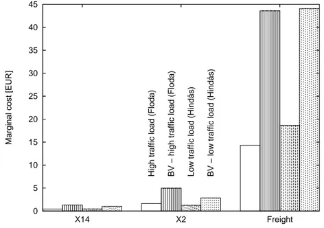
Figure 4 shows the estimated yearly marginal cost for one person at a distance of 50 m from the railway line for the two case studies presented in section 3.2. The figure includes two approaches with which to derive this cost: (i) directly from the estimation of noise level via Figure 3 and (ii) indirectly via Eq. (2). The parameter N in Eq. (2) is the maximum level, but to be able to make a comparison it is assumed to be the equivalent level (LA,Eq,24h) with and without the train at the point of reception. It is more difficult to work with the maximum level

since it does not change if the train is not the noisiest along the line and is not affected by the volume of traffic. Since the maximum level is higher than the equivalent level, the marginal cost is underestimated when using this approach.

The marginal cost is calculated at a distance of 50 m from the track in a position without significant screening for the three different trains shown in Table 2. The change in A-weighted equivalent noise level is calculated in Figure 2. While this change is not attributable to distance from the track, the absolute level is, which is why we assume a distance of 50 m.

(14)

Marginal cost calculated with Eq. (2) becomes 50 − 100% higher than with the direct method. Note too that the marginal cost per person and year 50 m from the track becomes the same in size for both high traffic (Floda) and low traffic (Hind˚as). This is due to the fact that a train makes smaller changes to a noise level that is already high because of other traffic, but the smaller change incurs a higher monetary value since the noise level is high. Put another way; since the change in cost increases substantially for higher sound levels (see Figure 3), even a small change in effect on the equivalent noise level in a noisy place will incur a cost.

0 5 10 15 20 25 30 35 40 45 Freight X2 X14

Marginal cost [EUR]

High traffic load (Floda) BV − high traffic load (Floda) Low traffic load (Hindås) BV − low traffic load (Hindås)

Figure 4: Calculated marginal cost per year for one inhabitant at a distance of 50 m from the railway.

5.2 Marginal cost and infrastructure charge

The social cost of a marginal noise increase can be calculated by combining the estimated marginal cost with the number of exposed. Let g(L) denote the distribution function for the number of exposed at different noise levels. The marginal cost (MC) for noise at a given noise level Lican thereby be written as;

MC(Li) = f (Li)g(Li). (4)

Society’s total marginal noise cost (T MC) can then be calculated as

T MC = Z _∞

π f (L)g(L)dL, (5)

whereπis the lower limit under which noise is not expected to cause annoyance.

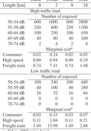
Table 3 below gives a calculation example of the marginal of driving one extra train of type X14 (commuter train), X2 (high speed) and freight train through the area. The link is entirely fictitious and consists of, apart from

(15)

departure and arrival points, a small urban area between two sparsely populated areas (denoted rural). The total number of exposed in each noise level category is estimated from calculations using NMT96 and assuming an even population distribution throughout the affected areas. The number of exposed is fewer for the low traffic load example since the total noise source strength is lower causing lower noise level at the same distance from the railway compared to the high traffic load area, which is illustrated in Figure 5.

55 dB 60 dB

low traffic load high traffic load

railway line

Figure 5: Sketch of the effect of changing the traffic volume in the example. The noise contours move outward to include more dwellings when the traffic is increased.

The results of the highly simplified model show, in line with the results in Figure 2, significant differences in marginal noise between the X14, X2 and freight trains and between low and high traffic loads. The table also shows the effect of noise on the marginal cost calculation. The speed is assumed to be the same for X14 and freight trains, which is not realistic, but since the effect of speed on the estimations is not significant we have, for the sake of simplicity, chosen to let the speed be the same.13

Table 3 also shows estimations of differentiated noise charges in e/km (2006 price level). The large difference between noise charges for commuter and freight trains can be traced to the difference in marginal noise addition. What is also interesting is that the charge through the low traffic load area is higher than through the high traffic load area. The effect of higher marginal noise at a lower noise level is thus stronger than at a higher noise level. It is also worth noting that the charges are in line with the ranking of disturbance level for passenger and freight trains; that is, people feel more disturbed by noise from freight trains.

The marginal cost is directly proportional to the number of exposed. Doubling the population in the area will double the marginal cost per km through it (under the assumption that the added population is evenly distributed). Note however that the marginal cost is not proportional to the total traffic. In the example above increasing the traffic from 39 trains per 24h to 190 (almost a 400% increase) lowers the marginal cost by approximately 65%, so the estimated marginal costs are less sensitive to changes in the total traffic volume.

(16)

Table 3: Example of noise charges for three train types Rural Urban Rural Total

Length [km] 8 2 8 18

High traffic load

Number of exposed 50-54 dB 600 1600 600 2800 55-59 dB 250 600 250 1100 60-64 dB 100 250 100 450 65-69 dB 40 80 40 160 70-74 dB 2 4 2 8 Marginal costa Commuter 0.02 0.24 0.02 0.05 High speed 0.09 0.94 0.09 0.19 Freight train 0.74 7.41 0.74 1.48 Low traffic load

Number of exposed 50-54 dB 100 240 100 440 55-59 dB 40 100 40 180 60-64 dB 16 32 16 64 65-69 dB 0 0 0 0 70-74 dB 0 0 0 0 Marginal costa Commuter 0.03 0.33 0.03 0.07 High speed 0.11 1.04 0.11 0.21 Freight train 1.49 13.99 1.49 2.88 a: e/km, 2006 price level.

5.3 Impact Pathway Approach

The Impact Pathway Approach (IPA) is a method that has been suggested for estimating the cost of noise (Metroe-conomica, 2001; Navrud, 2004).14 The method has been developed for energy externalities (ExternE, 2005) and is intuitive and easy to understand. In short, the method follows a “bottom-up approach”; that is, its starting point is the source of emission, and it estimates the propagation and final effects of the emission. These effects are then given monetary values and the social cost can be established.

IPA has been used in a several studies to estimate noise costs (Metroeconomica, 2001; Schmid and Friedrich, 2002; Bickel et al., 2002). The method is also advocated by St˚ale Navrud in his “state-of-the-art”-study of the evaluation and cost calculation of noise (Navrud, 2004). Another reason for using the method is that it cannot be assumed that individuals are aware of all the effects of noise exposure (Navrud, 2004), e.g., increased blood pressure. The monetary value that individuals either disclose through their decisions (RP) or state in questionnaires and interviews (SP) is therefore expected to underestimate the actual social noise cost. Lindberg (2003) compared the Swedish efforts to estimate social noise cost with the results from Schmid and Friedrich (2002) and found only small differences. However, Lindberg was of the opinion that this was probably due to “chance” (Lindberg, 2003).

14_{Most often termed “impact pathway approach”, and sometimes “damage function approach”, in the literature. For a run-through of the}

(17)

Even if IPA is intuitively appealing, there are several well known problems. The method builds on emission being measured with precision in terms of its spread and eventual effects. Data for the specific effects (e.g., health status) and preference estimations for the goods or populations is also necessary. Since this data is often lacking, the cost calculations will depend on assumptions regarding health data and how well BT functions in the specific case. This, together with the unreliability associated with the calculation of “dose-response”, results in great uncertainty in the estimations (Metroeconomica, 2001). The assumption that individuals are not aware of the various health risks can also be an issue. If there is general awareness of the risk of, e.g., increased blood pressure, IPA will mean a double counting of the social utility from reducing the noise level. It is therefore important to establish what individuals take into account when they state their WTP in practical decisions or as answers to hypothetical questions, something that has to be done empirically.

A general problem with IPA is the evaluation of the risk of death. The measure “value per statistical life-year” (VSLY), which is based on estimations of “value of a statistical life” (VSL), is used in IPA.15When using VSLY it is assumed that VSL diminishes with age (Hammitt, 2000; Alberini and Krupnick, 2002). A document from the European Commission on recommended values for reducing risk states that there is strong theoretical and empirical evidence that VSL diminishes with age (European Commission, 2000b), but Johansson (2002) showed that there is no strong theoretical evidence of VSL diminishing with age. Empirical support for the same also seems to be lacking (Aldy and Viscusi, 2007; Krupnick, 2007), something that users of IPA are often aware of (Bickel et al., 2002, p. 16).

6 Suggestions for a charging model

A noise charge for railway operators should be differentiated and reflect the actual differences in marginal costs for different trains, how the trains are driven, at what time of the day and on what stretches and so on. The desired differentiation is not always possible when implementing the charges according to the marginal principle, since it would be prohibitively costly to obtain the correct bases for exact differentiation. Therefore, there is a need to introduce a system that is implementable, given the existing knowledge level of the various marginal costs and taking into account the balance between the benefit of including the externality and the cost of calculating it.

In order to establish the size of the marginal cost of the noise to be included in the railway infrastructure charge, the following bits of information are needed;

1. the noise situation before the change,

2. how the noise situation is changing and

3. connection between the noise level and cost.

15_Let_δ_{denote the discount rate of interest; then the following relation applies (Alberini and Krupnick, 2002); V SL = V SLY}RT

(18)

It is natural to use the available noise calculation methods for noise from railway traffic (Harmonoise, NMT96) for the first two points. At best there is information on the noise situation before the change which will already be accessible in the form of noise maps where the levels are given as contours or colored areas. The change in the new trains can probably be calculated with good precision once and then be valid for the whole area. If, for example, the equivalent level increases by 0.1 dBA, then it will be applicable both near and far from the track and in screened areas as well. It would also be desirable to be able to distinguish between these in terms of their actual noise emission, e.g., in the form of a certification system. Operators who have invested in noise reducing technology should be charged less in such a system compared to those who have not invested in similar technology. The monetary evaluation of changed noise levels is also needed to estimate the noise component of the railway infrastructure charge. As seen in the calculation example in the Table 3, estimates for road traffic are used. Research shows that people are disturbed to varying degrees by road and rail noise and it can therefore be desirable to evaluate railway noise. Given the values that reflect the social marginal cost for railway noise, information on the noise levels at the exposed individuals’ houses is needed for calculation of the actual marginal cost. In principle, the sound level depends on the distance from the track plus any screening and land effects. In other words, points 1 and 3 above require geographic information (where houses are located, distance, possible noise screens, land quality and so on) and noise evaluation. For point 2 details are required for the train for which the railway infrastructure charge is to be calculated. If it is a known train type then a measuring method is already prescribed for example in de Vos et al. (2005). How the necessary input is connected is illustrated in the Figure 6.

Figure 6: Overview of information needed to estimate the noise component of the rail access charge (the marginal cost of noise).

An alternative that will reduce the amount of input data required for the calculation is to use the rule of thumb for how the population is distributed at various distances from the track. Noise calculation can then be made for a number of scenarios, e.g., built-up area with noise screens, countryside with soft arable land and the like.

(19)

A suitable basis for the development of such rules of thumb would be to make accurate case studies with noise maps and investigation of housing locations in several places. With these case studies as a starting point, one can compare the effects of different assumptions and rules of thumb and thus acquire an understanding of the loss of precision in the noise charges from these assumptions and rules of thumb.

7 Conclusion

This chapter makes suggestions for how marginal noise from trains can be calculated, discusses issues associated with the evaluation of noise, proposes a sketch of what is needed to include a noise component in the railway infrastructure charge and provides a calculation example with a noise charge. The estimated values in this chapter are only numerical examples and we would advise against their use in noise charges.16

Considering the sketch for the railway infrastructure charge in this chapter, we do not see the declaration procedure as a basis for collection of the railway infrastructure charges, as a problem. The information that rail authorities need from the operator is the stretch, train type, number of carriages and speed. The noise maps that are presently being produced as required by the Environmental Noise Directive of the European Commission (European Commission, 2002) will give the authorities the necessary information on noise level and the number of exposed. We consider that the greatest obstacle to an implementation of a noise charge in the near future is the lack of an estimated monetary value for railway noise. This value can be estimated, however, and is not an acceptable reason for rejecting the marginal cost principle.

Criticism has been aimed at the slowness of the work on reducing noise levels, especially on the emission side (see e.g., Kihlman, 2005b). Noise charges based on the marginal cost principle are a possible way of providing an incentive for those who cause the noise to reduce the “emission”. Even if a socially optimal noise level, and not a reduced noise level, is the primary objective of marginal cost pricing, today’s “zero price” of noise means that the marginal cost principle will make it costly to spread the noise and thereby provide an incentive to reduce the noise level. We, therefore, believe that a charge that reflects noise costs would be an effective means of reducing noise levels.

Bluhm and Nordling (2005) found no connection between railway noise and increased blood pressure, but several studies show a connection between noise disturbance and health levels (see Babisch et al., 2005). There-fore, there is support for the fact that a marginal noise increase leads to worsened health and a resulting social cost. Whether the individual takes this into consideration when evaluating noise (actual or hypothetical) is an issue of an empirical nature that must be investigated. As we do not believe that it is possible, in the short run, to estimate differentiated values for housing, workplace, school, recreation and so on, estimations should be based on housing in the future as well. The same applies to the possible differentiation between passenger and freight

(20)

trains. Differentiated estimations would probably be far too expensive today.

If rail authorities unilaterally internalized the railways’ externalities and based the railway infrastructure charge on the marginal cost principle, the resulting problem would be a possible distortion in the competitive climate. Notwithstanding, this is not a sustainable argument for excluding noise from the charge while e.g., wear and tear are included. We consider it better for all the externalities to be included and for the problem of the distortion of competition to be dealt with in another way. If the railways could solve the implementation issue and introduce a system based on the marginal cost principle, we believe it would probably result in political pressure for other transport modes to be embraced by the principle as well.

(21)

References

Alberini, A. and A. Krupnick: 2002, The International Yearbook of Environmental and Resource Economics 2002/2003, Chapt. Valuing the Health Effects of Pollution, pp. 233–277. Cheltenham, UK: Edward Elgar. Aldy, J. E. and W. K. Viscusi: 2007, ‘Age Differences in the Value of Statistical Life: Revealed Preference

Evidence’. Review of Environmental Economics and Policy 1(2), 241–260.

Andersson, H. and M. ¨Ogren: 2007, ‘Noise Charges in Rail Infrastructure: A Pricing Schedule Based on the Marginal Cost Principle’. Transport Policy 14(3), 204–213.

Andersson, H.: 2005, ‘The Value of Safety as Revealed in the Swedish Car Market: An Application of the Hedonic Pricing Approach’. Journal of Risk and Uncertainty 30(3), 211–239.

Atkinson, S. E. and R. Halvorsen: 1990, ‘The Valuation of Risks to Life: Evidence from the Market for Automo-biles’. Review of Economics and Statistics 72(1), 133–136.

Babisch, W., B. Beule, M. Schust, N. Kersten, and H. Ising: 2005, ‘Traffic Noise and Risk of Myocardial Infarc-tion’. Epidemiology 16(1), 33–40.

Banverket and Naturv˚ardsverket: 2002, ‘Buller och vibrationer fr˚an sp˚arbunden linjetrafik: Riktliner och till¨ampning’. Banverket (National Rail Administration) and Naturv˚ardsverket (The Swedish Environmental Protection Agency).

Bateman, I. J., R. T. Carson, B. Day, M. Hanemann, N. Hanley, T. Hett, M. Jones-Lee, G. Loomes, S. Mourato, ¨

Ozdemiro¯glu, D. W. Pearce, R. Sugden, and J. Swanson: 2002, Economic Valuation with Stated Preference Techniques: A Manual. Cheltenham, UK: Edward Elgar.

Bateman, I., B. Day, I. Lake, and A. Lovett: 2001, ‘The Effects of Road Traffic on Residential Property Values: A Literature Review and Hedonic Pricing Study’. Technical report, University of East Anglia, Economic & Social Research Council, and Univeristy College London.

Bickel, P., S. Schmid, and R. Friedrich: 2002, ‘Estimation of Environmental Costs of the Traffic Sector in Sweden’. Mimeo, Institut f¨ur Energiewirtschaft und Rationelle Energieanwendung (IER), Universit¨at Stuttgart.

Bluhm, G. and E. Nordling: 2005, ‘Health Effects of Noise from Railway Traffic - The HEAT Study’. Inter-Noise. Boverket: 2003, ‘Buller: Delm˚al 3 - Underlagsrapport till fördjupad utvärdering av miljöm˚alsarbetet’. Boverket,

Karlskrona.

Carlsson, F., E. Lampi, and P. Martinsson: 2004, ‘Measuring Marginal Values of Noise Disturbance from Air Traffic: Does the Time of Day Matter?’. Working Papers in Economcis 125, Dept. of Economics, Gothenburg University, Gothenburg, Sweden.

Carson, R. T., N. E. Flores, and N. F. Meade: 2001, ‘Contingent Valuation: Controversies and Evidence’. Envi-ronmental and Resource Economcis 19(2), 173–210.

Day, B.: 2001, ‘The Theory of Hedonic Markets: Obtaining Welfare Measures for Changes in Environmental Quality using Hedonic Market Data’. Economics for the Environment Consultancy, Mimeo.

de Vos, P., M. Beuving, and E. Verheijen: 2005, ‘Harmonised Accurate and Reliable Methods for the EU Direc-tive on the Assessment and Management of Environmental Noise – Final technical report’. Technical report. http://www.harmonoise.org.

Dreyfus, M. K. and W. K. Viscusi: 1995, ‘Rates of Time Preference and Consumer Valuations of Automobile Safety and Fuel Efficiency’. Journal of Law and Economics 38(1), 79–105.

European Commission: 1998, ‘White Paper on Fair Pricing for Transport Infrastructure Use’.

European Commission: 2000a, ‘Proposal for a Directive of the European Parliament and of the Council relat-ing to the Assessment and Management of Environmental Noise’. Technical Report COM(2000) 468 final, 2000/0194(COD), Commission of the European Communities.

(22)

European Commission: 2000b, ‘Recommended Interim Values for the Value of Prevent-ing a Fatality in DG Environment Cost Benefit Analysis’. mimeo, 08/06/04 available at: http://europa.eu.int/comm/environment/enveco/others/recommended interim values.pdf, 08/06/04.

European Commission: 2002, ‘Environmental noise directive 2002/49/EG’.

ExternE: 2005, ‘ExternE: Externalities of Energy. A Reserach Project of the European Union’. Internet, www.externe.info, 10/7/05.

Friedrich, R. and P. Bickel: 2001, Environmental External Costs of Transport. Heidelberg, Germany: Springer Verlag.

Hammitt, J. K.: 2000, ‘Valuing Mortality Risk: Theory and Practice’. Environmental Science & Technology 34(8), 1396–1400.

Hartung, C. F.: 2000, ‘Vibrations and external noise from train and track - a literature survey’. Report F227, Chalmers Solid Mechanics.

HEATCO: 2005, ‘Developing Harmonised European Approaches for Transport Costing and Project Assess-ment, Deliverable four - Economic values for key impacts valued in the Stated Preference surveys’. http://heatco.ier.uni-stuttgart.de, 8/29/07.

Imagine: 2005. http://www.imagine-project.org/.

Johansson, P.-O.: 2002, ‘On the Definition and Age-Dependency of the Value of a Statistical Life’. Journal of Risk and Uncertainty 25(3), 251–263.

Kahneman, D. and J. L. Knetsch: 1992, ‘Valuing Public goods: The Purchase of Moral Satisfaction’. Journal of Environmental Economics and Management 22(1), 57–70.

Kalivoda, M., U. Danneskiold-Samso, F. Kr¨uger, and B. Bariskow: 2003, ‘EURailNoise: a study of European priorities and strategies for railway noise abatement’. Journal of Sound and Vibration 267, 387–396.

Kihlman, T.: 2005a, ‘Developments in Environmental Noise Policies’. Budapest, pp. 35–40, Proceedings of Forum Acusticum. Paper 964-0.

Kihlman, T.: 2005b, ‘Developments in Environmental Noise Policies’. ForumAcusticum.

Krupnick, A.: 2007, ‘Mortality Risk Valuation and Age: Stated Preference Evidence’. Review of Environmental Economics and Policy 1(2), 261–282.

Lindberg, G.: 2003, ‘Marginella bullerkostnader: en genomg˚ang av SIKAs och V¨agverkets arbete samt analyser med effektkedjemetoden’. SIKA Rapport 2003:1, Bilaga 3, Trafikens externa effekter - Uppf¨oljning och utveck-ling 2002 - Bilagor, Stockholm, Sweden.

Lundström, A., M. Jäckers-Cüppers, and P. Hübner: 2003, ‘The new policy of the European Comission for the abatement of railway noise’. Journal of Sound and Vibration 267, 397–405.

Metroeconomica: 2001, ‘Monetary Valuation of Noise Effects: Final Draft Report’. Mimeo, May, Preparde for The EC UNITE Project.

Nash, C.: 2005, ‘Rail Infrastructure Charges in Europe’. Journal of Transport Economics and Policy 39(3), 259–278.

Naturv˚ardsverket: 1996, ‘Buller fr˚an sp˚arburen trafik – Nordisk Ber¨akningsmodell’. Rapport 4935, Naturv˚ardsverket (Swedish Environmental Protection Agency), Stockholm, Sweden.

Navrud, S.: 2004, ‘The Economic Value of Noise Within the European Union - A Review and Analysis of Studies’. Mimeo.

Nijland, H. A., E. E. M. M. Van Kempen, G. P. Van Wee, and J. Jabben: 2003, ‘Costs and Benefits of Noise Abatement Measures’. Transport Policy 10(2), 131–140.

(23)

¨

Ohrstr¨om, E., A. Sk˚anberg, L. Barreg˚ard, H. Svensson, and P. ¨Angerheim: 2005, ‘Effects of Simultaneous Expo-sure to Noise from Road and Railway Traffic’. Inter-Noise.

Petersson, M.: 1999, ‘Noise-related roughness of railway wheels - testing of thermomechanical interaction be-tween brake block and wheel tread’. Licentiate thesis, Chalmers University of Technology. Chalmers Solid Mechanics.

Plovsing, B. and J. Kragh: 2000a, ‘Comprehensive Outdoor Sound Propagation Model. Part 1: Propagation in an Atmosphere without Significant Refraction’. Delta report AV 1849/00, Delta, Lyngy, Denmark.

Plovsing, B. and J. Kragh: 2000b, ‘Comprehensive Outdoor Sound Propagation Model. Part 2: Propagation in an Atmosphere with Refraction’. Delta report AV 1851/00, Delta, Lyngy, Denmark.

Prop. 1997/98:56: 1998, ‘Government bill 1997/98:56: Transportpolitik f¨or en h˚allbar utveckling’. Government bill by the Swedish Government.

Rosen, S.: 1974, ‘Hedonic Prices and Implicit Markets: Product Differentiation in Pure Competition’. Journal of Political Economy 82(1), 34–55.

Rothengatter, W.: 2003, ‘How good is first best? Marginal cost and other pricing principles for user charging in transport’. Transport Policy 10(2), 121–130.

Sansom, T., C. A. Nash, P. J. Mackie, J. Shires, and P. Watkiss: 2001, ‘Surface Transport Costs and Charges: Great Britain 1998’. Final report, Institute for Transport Studies, University of Leeds, UK.

Schmid, S. A. and R. Friedrich: 2002, ‘External costs of transport noise. a bottom-up appraoch’. Inter-noise 2002. SIKA: 2002a, ‘Nya banavgifter? Analys och f¨orslag’. SIKA Report 2002:2, SIKA (Swedish Institute for Transport

and Communications Analysis) and Banverket, Stockholm, Sweden.

SIKA: 2002b, ‘ Översyn av samhällsekonomiska kalkylprinciper och kalkylvärden p˚a transportomr˚adet’. SIKA Report 2002:4, SIKA (Swedish Institute for Transport and Communications Analysis), Stockholm, Sweden. SIKA: 2008, ‘Samhällsekonomiska kalkylprinciper och kalkylvärden för transportsektorn’. SIKA PM 2008:3,

SIKA (Swedish Institute for Transport and Communications Analysis), Stockholm, Sweden.

Söderström, L.: 2002, Öresundsförbindelse med ett hinder mindre: Effekter p˚a integrationen vid avgiftsfrihet, Chapt. Priser och samhällsekonomi, pp. 35–47. Lund, Sweden: Öresundsuniversitetet.

UIC: 2005. http://www.uic.asso.fr/environnement/Railways-Noise.html. International Union of Railways. Wall, R.: 2005, ‘Buller - En förstudie om samhällsekonomisk värdering av buller med direkt ljudmätning’. Mimeo,

V¨agverket, Borl¨ange, Sweden.

Wilhelmsson, M.: 1997, ‘Trafikbuller och fastighetsv¨arden - en hedonisk prisstudie’. Meddelande 5:45, Division of Building and Real Estate Economics, Royal Institute of Technology, Stockholm, Sweden.

Marginal cost pricing of noise in railway infrastructure