Determinants of Capital Structure in Family Firms

(1)

Determinants of Capital

Struc-ture in family firms

An empirical evidence from OECD countries

Master’s thesis within Business Administration, International Financial Analysis

Author: Ahmed Akbarali 851122 Awambeng Foma 910914

(2)

Master’s thesis within Business Administration, International Financial Analysis

Title: Determinants of Capital Structure in family firms

Author: Ahmed Akbarali 851122

Awambeng Foma 910914

Tutor: Jonas Dahlqvist

Date: September 2015

Subject terms: Capital structure, Family firms, OECD countries, Financial Deci-sions

Abstract

Most firms are using optimal combination of equity and debt so as to maximize firms value and the wealth of the shareholders. To achieve all these, firms should be aware of the factors that influence the capital structure decisions.

Previous empirical studies attempted to explain what determines the choice of capital structure in firms. The focus was on firms in general without categorizing family firms and non-family firms. The primary objective of this study is to examine what determines the capital structure of family firms in OECD countries.

Amadeus database was used to obtain the data needed for the statistical analysis. Measures for firm-specific characteristics were calculated based on the previous stud-ies. The study was conducted over a period of 9 years from 2005-2013. Dataset com-prised of 95 family firms resulting in 850 observations.

The results from the study indicate that the capital structure for family firms in OECD countries is influenced by profitability, asset tangibility, growth, size, debt tax shield , non-debt tax shield and liquidity. Both pecking-order theory and trade-off theory explain the capital structure of family firms.

(3)

1 INTRODUCTION ... 3

1.1 BACKGROUND... 3 1.2 PROBLEM STATEMENT ... 4 1.3 PURPOSE ... 4 1.4 RESEARCH QUESTIONS ... 4

2 THEORETICAL FRAME OF REFERENCE ... 5

2.1 CAPITAL STRUCTURE ... 5

2.2 THEORIES OF CAPITAL STRUCTURE ... 5

2.2.1 MODIGLIANI MILLER THEORY ... 5

2.2.2 STATIC TRADE-OFF THEORY ... 6

2.2.3 PECKING-ORDER THEORY... 7

2.3 DETERMINANTS OF CAPITAL STRUCTURE ... 8

2.3.1 Firm Profitability ... 8

2.3.2 Firm Size ... 8

2.3.3 Firm Growth Opportunities ... 9

2.3.4 Asset Tangibility ... 9 2.3.5 Tax Shields ... 10 2.3.6 Firm Liquidity ... 10

3 METHOD ... 11

3.1 Research Design ... 11 3.2 Research Strategy ... 11

3.3 Sampling and Sample size ... 11

3.4 Description of Variables ... 12

3.4.1 Dependent Variable ... 12

3.4.2 Independent Variables ... 12

3.5 Data Analysis Techniques ... 13

3.6 Pooled Regression Model ... 13

3.7 Random Effects Model ... 14

3.8 Limitations ... 14

4 EMPIRICAL FINDINGS ... 15

4.1 Descriptive Statistics ... 15

4.2 Correlation Analysis ... 17

4.3 Pooled Regression Model ... 17

4.4 Panel Regression Model with Random Effects ... 20

5 ANALYSIS ... 22

5.1 Profitability ... 22

5.2 Asset Tangibility ... 22

5.3 Growth ... 23

5.4 Size ... 23

5.5 Debt -Tax Shield... 23

5.6 Non-Debt Tax Shield ... 24

5.7 Liquidity ... 24

6 DISCUSSION ... 25

(4)

6.2 Limitations ... 26

6.3 Further Research ... 26

List of references ... 27

Tables

Table 3.4 Independent and dependent variables………....13

Table 4.1 Descriptive Statistics………15

Table 4.2 Correlation Matrix……….17

Table 4.3 Pooled Panel Least Squares Results………...18

Table 4.4 Random Effects Regression Model Results………21

Appendix

Descriptive Statistics ... 31

Correlation Matrix………....31

Pooled Regression Model 1………...32

Pooled Regression Model 2………...……32

Random Effects Model 3………...….33

Random Effects Model 4………...……….34

Hausman Test on Model 3………...34

(5)

1 INTRODUCTION

This chapter aims to introduce to the reader the determinants of capital structure of family firms in OECD countries. The general background, problem statement, purpose of the study, and research questions will be presented.

1.1 BACKGROUND

Since the classic work by Modigliani and Miller (1958) where they described how and why the capital structure is irrelevant, capital structure has been one of the most widely discussed topics in finance among academics. A number of the previous studies focused on analysing publicly traded firms or non-family firms while most of the studies carried out failed to examine the capital structure in the context of family firms.

According to European Family Businesses (2013), “A firm of any size is a family business if:

The majority of decision making rights are in the possession of the natural person(s) who established the firm. (Family firm institute) or in the possession of the natural person who has/have acquired the shared capital of the firm or in the possession of their spouse, parent, child or children. Also the majority of the decision making rights are direct or indirect and at least one representative of the family or kin should be formally involved in the governance of that firm. Finally, listed companies meet the definition of fairly firm if the person who established or acquired the firm (shared capital) or their families or descendants possess 25% of the decision-making rights mandated by their share of capital.” Kashyap and Zingales (2010) pointed out that, the financial crisis of 2008 has contributed to the increased attention towards capital structure decisions, as it highlighted the importance of deviations from Modigliani and Miller’s irrelevance theorem. A number of previous studies tried to find out what factors affect firms’ financial decisions that resulted to two main theories; pecking- order theory, which suggest that companies prefer the cheapest source of funding, and the trade-off theory that explained that the choice of capital structure is a result of a trade-off between the benefits of debt, such as the debt-tax shield, and the cost of debt, including bankruptcy cost and cost of financial distress (Nilssen, 2014). However, Myers (2014) argued that companies will prefer internal to external funding and debt over equity because of the information asymmetry.

The two theories of capital structure were set as the basis for number of studies that have been conducted later trying to determine which model best explains the choice of financing and what factors influence the capital structure decisions in the firms. Recently, researchers (e.g Ampenberger et at, 2009; Romano et al, 2001) have strived to determine the most important determinants of capital structure and how it varies across companies and across countries.

(6)

1.2 PROBLEM STATEMENT

Firms cannot run, grow and expand their businesses without capital (Pike & Neale, 1993). The question comes, how do firms finance and structure their capital? A number of studies have been conducted for the past five decades but the focus was on non-family firms. One of the most important decisions any firm has to make is concerning the combination of debt and equity for a firm, which represents the firm’s target capital structure. There are number of factors which influence the capital structure of a company. All firms should be aware of these factors in order to determine the target that will be based on the choice of capital. Previous studies identified specific characteristics of capital structure. This study has chosen seven characteristics namely; firm’s profitability, firm’s size, firm’s growth opportunities, asset tangibility, tax shields, firm’s liquidity and business risk. The effect of these factors will be examined based on leverage ratios. The study will seek to examine how these determinants influence the capital structure of family firms in nine OECD countries obtained in global family index of St. Gallen University in Switzerland. This research analyses the explanatory power of the established theories and firm’s specific factors from the literature in explaining the choice of capital structure across nine OECD countries family firms. We believe that the capital structure of family firms to be a financial complex issue as the determinants of capital structure affect the financial decisions of the firms.

1.3 PURPOSE

The purpose of this study is to identify the factors that influence capital structure and how they affect the family firms financing decisions in the OECD countries. In addition to this study aims at testing how the identified determinants of capital structure are affecting OECD family firms. Finally this research will verify whether the general capital structure theories predict similar relationships between the capital structure and its determinants in OECD family firms.

1.4 RESEARCH QUESTIONS

To achieve the purpose of this study, the following questions are presented; 1. What are the determinants of capital structure for family firms?

2. How do these determinants affect the capital structure of family firms? 3. Do the capital structure theories predict similar relationship between capital

(7)

2 THEORETICAL FRAME OF REFERENCE

The following chapter provides an overview of theoretical frame of reference relating to capital structure in general, theories of capital structure, and determinants of capital structure.

2.1 CAPITAL STRUCTURE

Capital structure of a company is the way a company finances its assets. This can be done by either debt or equity or a combination of both at different stages of the firm (Borad, 2013). The capital structure of some firms is made more of debt or equity. Number of capi-tal structure theories tried to establish a relationship between financial leverage that is the proportion of debt in a company’s capital structure with its market value. The static trade-off theory and the pecking order theory were developed to provide the conceptual frame-work for the capital structure theory. Due to the fact that the trade-off theory is an exten-sion of the Modigliani Miller (MM) theory, this theory will be discussed briefly in this study this study, so that the reader can understand the whole concept of capital structure theory.

2.2 THEORIES OF CAPITAL STRUCTURE

There are three theories related to capital structure of the firms developed by different authors.

2.2.1 MODIGLIANI MILLER THEORY

Modigliani and Miller proposed this theory during the 1950s (Borad, 2013). The Modigliani-Miller approach is very much similar to the net operation income approach (Borad, 2013). The MM theory suggests the capital structure irrelevancy theory which suggest that the capital structure of a firm is irrelevant to the valuation of a firm (Borad, 2013; Frank & Goyal, 2005) and whether the firm is highly leveraged or has lower debt components in the financing mix, this has no bearing on the value of the firm. Furthermore, the Modigliani Miller theory states that the market value of a firm is influenced by its future growth prospects apart from the risk involved in the investment (Myers, 1984). According to the MM theory, the value of a firm is not dependent on the choice of capital structure or financial decision of the firm (Borad, 2013). Furthermore the theory advocates that companies with high growth prospects also experience a high market value and eventually high stock prices. If investors can’t forecast or perceive attractive growth prospects in a firm, the market value of the firm would not be that great.

Assumptions of the MM theory are: • There are no taxes.

• No transaction cost for buying and selling securities as well as no bankruptcy cost.

• There is symmetry of information. This implies that investors will have access to some information to ensure some corporation and some rational behaviour among investors.

• Cost of borrowing is the same for investors and firms as well. • Debt financing does not affect companies (Myers, 1984)

(8)

These assumptions are not realistic as the views proposed in MM propositions, that altering financial decisions adds no value value to the firm, triggered a significant number of studies to be carried out in capital structure theory (Ngugi, 2008). As a result of these studies, the static trade-off theory and pecking-order theory were developed to provide a conceptual framework for capital structure theory.

2.2.2 STATIC TRADE-OFF THEORY

One of the limitations of the MM theory is that it has some unrealistic assumptions. The static trade-off theory came from Modigliani and Miller (1963) who suggested that optimal capital structure is all debt due to the benefit of tax deductibility of interest expense (Luambano, 2012). However, Stiglitz (1972) and Castanias (1983) argued that, despite the tax incentive of debt finance, higher leverage increases bankruptcy risks and such risks ought to be considered in deciding financing mix. As a result, trade-off theory conceptualizes that capital structure decisions entail attaining a balance between benefits of debt, agency cost and bankruptcy risks. Generally, the static trade-off theory states that, firms pursue a target capital structure that trades-off the effects of tax-benefits of debt, agency costs and bankruptcy costs (Huang & Song, 2006). This implies that; firms are expected to hold higher debt as long as benefits of debt exceed bankruptcy costs. Based on agency costs, the trade-off theory posits that debt is preferred by shareholders as a disciplining tool for management. Higher debt level would reduce conflict of interest as it leaves little free cash-flows available for managers to utilise for their personal uses. Sometimes, agency costs are considered as a separate theory but Huang and Song (2006) suggested that agency-cost-based models are only a different perspective of the trade-off theory.

IMPLICATION ON FAMILY FIRMS

As seen already in the paragraph above, the higher the debt level the higher the financial risk level consequently, the likelihood of bankruptcy cost in an attempt to relate the MM theory with family firms, according to Vieira (2013) family firms are more adverse to risk as well as could easily lose control than their counterparts and therefore try to avoid debt in their capital structure (Storey, 1994). By nature, family firms have long term perspective and as well as the desire to pass the firm on to succeeding generations. In addition there is no way for the capitalist to use portfolio reasoning. They only have one firm which puts a premium on survival over profitability of the firm. The concern for maintaining the family reputation and guaranteeing a save employment opportunity for family members (Stein, 1989; Anderson et al, 2003; Vieira, 2013) can encourage family firms avoid leverage as well as violations of debt covenants (Principe et al, 2008) family firms desire to maintain majority of ownership as well as a dominant position and control making the family firms disposed to limited capital leading to high risk of low or insufficient liquidity.

While the trade-off orders theory suggests an optimal level of debt that maximises a firm’s value and minimises the cost of capital by balancing the tax benefits and cost of bankruptcy, on the contrary the Pecking order approach advocates hierarchy of funding sources according to its cost as oppose to optimal capital structure of the trade-off theory.

(9)

2.2.3 PECKING-ORDER THEORY

Effecient financial management and the characteristics that affect their capital structure are important for both family and non-family firms in obtaining the best operational performance possible. Inadequate understanding may lead to incorrect decisions regarding the capital structure for firms and these can probably lead to financial distress and bankruptcy. Among the numerous works available on capital structure is the Pecking-order theory (Utama, 2013). The pecking-order theory is among the most influential and relevant theory in the study of corporate leverage. According to the theory there is no target capital

structure. Therefore, family firms would like to maintain ownership and majority of the market shares, make them prefer internal to external financing (Akbar, 2013; Vieira, 2013). Generally, the pecking-order theory is based on the asymmetric information between firms’ management (insiders) and potential investors (outsiders). It argues that a firm’s management is assumed to have more information about the firm’s value than potential investors, which leads investors to demand premium for the asymmetric information whenever they invest in the firm (Myers & Majluf, 1984). For financing purposes, firms prefer internal sources of fund, then less risky debt, followed by risky debt while equity finance ranks last in preference (Fama & French, 2002). According to the pecking-order theory, businesses would adhere to hierarchy of financing sources when available debt is preferred over equity in the case of external financing. Akbar (2013) argued that, pecking-order theory was first suggested in 1961 by Donaldson and it was modified by Myers and Majluf (1984).

The theory suggests that there are three sources of funding available to firms; retain earnings, debt and equity. Equity is subject to serious adverse selection problem, while debt has only a minor adverse selection problem and retain earnings has no adverse selection problem (Akbar, 2013).

Pecking-order theory point of view of outside Investor

Equity is strictly riskier than debt and both have an adverse selection risk premium. But the premium is greater than equity forcing an outside investor to demand a high rate of return on equity than on debt (Myers and Mayluf, 1984). This is because according to the authors, there are three sources of funding available to firms: retained earnings, debt and equity. Retained earnings have no adverse selection problem (Frank & Goyal, 2003). From the point view outside investor, equity is a little more risker than debt with both having an adverse selection premium; and the premium is large on equity (Frank & Goyal, 2003). This implies that an outside investor will demand higher rates of return on equity than on debt. Point of view or perspective of Insider

From the perspective of the pecking-order theory, retained earnings are better sources of finance compared to debt and debt is a better deal than equity financing. Accordingly, the firm if possible should fund all projects using retain earnings (Myers, 1984; Akbar, 2013). The theory goes further to make predictions about the majority and priority structure of debt. Securities with the lowest cost should be issued prior to securities with higher information cost, which implies that short term debt should be exhausted before long term debt (Akbar, 2013). If retained earnings become inadequate then the firm regardless of whether it is a family or a non-family firm should make use of debt financing (Frank & Goyal 2003). If a firm is operating normally, equity may not be the best option.

(10)

Pecking-order theory and Family Firms

Relating the pecking-order theory with family firms, Romeo et al (2000) conducted a study of capital structure decisions for family firms based on a questionnaire sent to a number of Australian family firms. Based on the results, it was realised that small family firms’ debt is significantly related to the size of the firm, family control, business planning and the business objectives. The findings of the study were that the older the business owner, the lower their preference for equity. According to these findings, the pecking order hypothesis provides a very useful and relevant explanation for family business financing decisions (Vieira, 2013). Furthermore Vieira (2013) argued that, in the context of the pecking-order theory, having more cash (cash and marketable securities) reduces the need to borrow. Of course one can deduce a negative correlation between debt and cash availability. As a result of the fact that family firms are more risk averse compared to non-family firms and even more specifically to the risk of financial distress (Zhou, 2012), the family firms tend to strengthen their relationship and depend more on internal funds for additional growth.

2.3 DETERMINANTS OF CAPITAL STRUCTURE

2.3.1 Firm Profitability

There exist some ambiguity in the theoretical relationship between leverage and profitability. The pecking-order theory depicts leverage as having a negative relationship with profitability, while the trade-off theory suggests a positive relationship. According to the pecking-order theory with an increase in profits, sufficient internal funds become more available and reduces the need for external financing for firms. Therefore leverage is expected to have a negative relationship with profitability, while on the other hand, the trade-off theory advocates that with an increase in profits since the risk of bankruptcy falls while income shield taxes increase. But leverage may be forced to increase with profits since the firm will try to balance both. A study by Gungoraydinoglu and Öztekin (2011) found a positive relationship between profitability and leverage in countries where creditor’s rights are protected. And there exist a negative relationship between leverage and profitability.

Based on the analysis above, we hypothesize that profitability is negatively related to leverage for family firms in OECD countries as described by pecking-order theory. Hence: H1: Profitability is negatively related to leverage for family firms in the OECD countries. 2.3.2 Firm Size

Based on the both pecking-order and trade-off theories, there exist both positive and negative relationship between the size of the firm and the leverage. Trade-off theory depicts a positive correlation between size and leverage. It suggests that larger firms are, on average, more diversified and have low bankruptcy risk. This facilitates the firm’s ability to access debt finance and hence a positive relationship exists between size and leverage. As a result of the fact that larger firms disclose more information to outsiders than smaller firms, the larger firms have low information asymmetry compared to smaller firms (Rajan & Zingales, 1995). Therefore large family firms are supposed to have at their disposal more equity than debt due to the low asymmetry information cost advantage they have. According to De Jong et al (2008), the authors realised that the size of a firm positively affects leverage. Moreover Rajan and Zingales (1995), Huang and Song (2006), and Kimura

(11)

(2011), had similar results. But Titman and Wassels (1988) found contrary views where they discovered that the firm’s size has a negative relationship with the leverage. Even though general opinion accepts that size is positively correlated to leverage, but there could be circumstances where the reverse is true and this cannot be completely rejected.

We hypothesize that leverage is positively related to size for family firms in OECD countries as predicted by trade off theory. Hence:

H2: Leverage is positively related to size for family firms in the OECD countries. 2.3.3 Firm Growth Opportunities

In general, firms with high growth prospects will require more funding than firms with low growth prospects. The pecking-order theory suggests that firms would need external funds to finance investment projects as they will not be able to finance all other investments opportunities with internal funds, Smith (2010). According to the pecking-order theory, it predicts a positive relationship between growth and leverage. But agency cost theory on the contrary postulates an opposite relationship. According to the agency cost theory, managers try to maximise personal utility at the expense of shareholders by avoiding the use of debt because debt acts like a disciplining tool which reduces free cash flow (Kayo & Kimura, 2011). Therefore, leverage decreases with an increase in growth opportunities, thus, a negative relationship between the two. Looking at an empirical study carried out by Huang and Song (2006) and De Jong et al (2008), they realised that levels decreased with increased in growth opportunities possible reason being that firm avoided the transfer of wealth from shareholders to creditors and failed to implement future profitable investment, on the contrary another study conducted by Rajan and Zingales (1995) found growth opportunities being positively correlated to leverage. This provides evidence as to the fact that there is no consensus as to the specific relationship between growth opportunities and leverage.

As such, we hypothesize that there is a positive correlation between firms’ growth and leverage for family firms in OECD countries as pointed out by pecking-order theory. Hence:

H3: Growth is positively correlated to leverage for family firms in the OECD countries. 2.3.4 Asset Tangibility

Prediction by the trade-off theory suggests a positive relationship between asset tangibility and leverage. According to the theory, fixed assets are treated as security or use as collateral to lenders. If a firm defaults payment of debt, the assets are realised by lenders as compensation, Smith (2010). The tendency for a firm with tangible assets to hold more debt because an increase in firm’s tangible asset will increase its borrowing capacity. The agency theory holds that shareholders can invest in projects which are at the interest of the firm at the lenders expense. So larger tangible assets are a proof to lenders that there is low agency cost in the firm (Huang & Song, 2006). All in all firms with larger tangible assets are expected to hold more debt compared to firms with low tangible assets. Empirical research pointed out that there is a positive relationship between leverage and asset tangibility. This was evident in a study of 42 countries De Jong et al (2008) where it was realised that asset tangibility is positively related to leverage. But in another study, Alves and Ferreira (2011) claimed that asset tangibility decreases with short term debt and increases with long term debt. In countries with strong creditor rights, Gungoraydinoglu (2011) found that there

(12)

was a weaker positive relationship between leverage and asset tangibility. But majority of the studies found asset tangibility positively related to leverage.

Based on the analysis above, we hypothesize that positive relationship between leverage and asset tangibility exists for family firms in OECD countries, as suggested by trade-off theory. Hence:

H4: Leverage is positively related to asset tangibility for family firms in the OECD countries.

2.3.5 Tax Shields

Tax shields are categorized as debt-tax shield and non-debt tax shield. A debt-tax shield can be defined as an interest deductibility of debt while non-tax shield is deduction for depreciation and investment credits (Delcoure, 2007). The trade-off theory suggests that firms hold debt levels which are minimised by bankruptcy risk. As a result, debt levels increase as long as debt benefits outweigh the bankruptcy risk otherwise it drops. The trade-off theory predicts a positive correlation between debt-tax shield and leverage. Huang and Song (2006) argues that non debt-tax shields are assumed to be perfect alternatives debt-tax shields. Therefore, an increase in non-debt tax shields would result in low debt preference. According to Delcoure (2007), non-debt tax shields positively affect debt and also that debt–tax shield is positively related to leverage for some West and Eastern European countries. But De Jong et al (2008) found a weak positive correlation of debt-tax shields to leverage in a random sample of 42 countries around the world.

Based on above analysis, as described by trade-off theory and other empirical studies, we hypothesize that leverage is positively related to debt-tax shield and negatively correlated to non-debt tax shield. Hence:

H5: Leverage is positively related to debt-tax shield for family firms in the OECD countries.

H6: Leverage is negatively correlated to non-debt tax shield for family firms in the OECD countries.

2.3.6 Firm Liquidity

Firm’s liquid assets have a high influence in the financial decisions. With the trade-off theory, higher liquidity signifies strong financial health for a firm and this means low risk of default and bankruptcy. But an increase in firm’s liquidity could also be looked upon as an increase in high debt levels as this increases the firm’s capacity to borrow (Smith, 2010). Under contrary, the pecking-order theory suggests an inverse relationship between liquidity and leverage. According to the pecking-order theory, high liquidity would imply sufficient internal sources are available for financing as a result, this would enable the firm to avoid external financing leading to low preference for debt financing when firm’s liquidity is high(Smith, 2010). The empirical evidence supports and at the same time opposes the view that positive relationship exists between firm’s liquidity and leverage. Previous studies depict that leverage is positively related to firm’s liquidity.

We hypothesize that leverage is positively related to firms’ liquidity as described by trade-off theory. Hence:

(13)

3 METHOD

In this chapter the research design, research strategy, sampling and sample size will be outlined. Data analysis techniques, description of variables, the use of pooled regression model and random effect model, and limitations of the study are considered.

3.1 Research Design

Overall plan for data collection and analysis strategy that will be applied in this study are described in this section. The cause and effect relationship equally exist between capital structure and its determinants (Kayo & Kimura, 2011). This study applies the same explanatory research design as Saunders et al (2007) suggested that studies which seek to establish causal relationship between variables should adopt explanatory design. However, a deductive approach was also adopted as the cause and effect relationship are explained on basis of existing pecking-order and trade-off theories. A deductive approach is concerned with developing a hypothesis or hypotheses based on existing theory and designing a research strategy to test the hypothesis (Wilson, 2010). This approach is concerned with deducting conclusions from premises or propositions. Deduction begins with an expected pattern that is tested against observations (Babbie, 2010).

3.2 Research Strategy

Due to the fact that secondary data was available to conduct this study, archival research strategy was applied. This should be most suitable for the research simply because, in order to establish relationship between capital structure and its determinants, analysis of past fi-nancial data is required. Myers and Mayluf (1984), Rajan and Zingales (1995), Huang and Song (2006), and Decloure (2007) applied similar strategy successfully in their studies. As we want our study to be performed on a continuous basis, this necessitated the use of sec-ondary data. This type of data permits us to compare financial data of family firms for dif-ferent countries all together at once. The use of secondary data puts our study on a positive research position, as it is assumed that firm’s financial statements are accurate but while in reality they may not be as accurate as such.

3.3 Sampling and Sample size

The sample frame used for this research is the financial statements of family firms in the OECD countries. In this regard the research collected secondary data, financial statements of family firms were downloaded from Bureau van Dyck Amadeus database in order to ex-amine the effect of determinants of capital structure. Amadeus database has an extensive coverage of large, medium, and small enterprises ( the mean asset size is 147 million Euro). We focused on consolidated statements of large and listed family firms. This study used a random sampling selection technique in selecting sample size. Random selection is the best method to use here in order to reduce biasness in the study, and to ensure that the study collects the most relevant data that reflects the population. The sample size of our study was 95 family firms randomly selected from nine OECD countries namely France, Germa-ny, Italy, Netherlands, Portugal, Spain, Sweden, Switzerland and United Kingdom. Only family firms with available data and financial statements publicly published were considered in this study. This selection was done because it is relatively easier to obtain financial in-formation required to test variables as it is legally mandatory for all listed companies to

(14)

publish their financial statements. This study covered a period of nine years, from 2005 to 2013 as it was possible to obtain financial annual reports for all sample.

3.4 Description of Variables

3.4.1 Dependent Variable

In this study, the capital structure was regarded as effect caused by its determinants, then it is a dependent variable. In measuring capital structure, the most widely used method is to proxy it with leverage ratios (Luambano, 2012). We used two leverage ratios; the ratio of total debt to total asset, and the ratio of total liabilities to shareholders’ equity plus total lia-bilities. These leverage ratios were used because they provide good results when used by Huang and Song (2006), other leverage ratios have limitations.

3.4.2 Independent Variables

The determinants of capital structure are regarded as independent variables in this study. We used profitability, firm size, firm growth opportunities, asset tangibility, tax shields and firm liquidity, as independent variables as applied by Luambano (2012).

Profitability

To establish specific relationship between profitability and leverage, profitability is defined as the ratio of operating profit before interest and tax to total assets as applied by Huang and Song (2006).

Firm Size

The proxy for size in this study is natural logarithm of sales as described by Nilssen (2014) in her research on Norwegian firms.

Firm Growth Opportunities

Firm growth is proxied by the percentage change in sales over the year as applied by Chakraborty (2010) in the study of capital structure in developing countries.

Asset Tangibility

To study the effect of asset tangibility on leverage, we define asset tangibility as a ratio of net fixed assets to total assets as applied by De Jong et al (2008).

Tax Shields

For testing purposes, this study defines debt-tax shield as effective tax rate while non-debt tax shield is proxied by depreciation and amortization of the fixed assets as applied by Smith (2010).

Firm Liquidity

The firm liquidity is defined as the ratio of working capital to total assets as applied in Smith (2010).

(15)

Table 3.4 Independent and dependent variables

Variable Symbol Measure (Proxy)

Leverage 1 LEV 1 Total Debt

Total Assets

Leverage 2 LEV 2 Total Liabilities

Shareholders′_{𝐸𝐸𝐸𝐸𝐸𝐸𝐸𝐸𝐸𝐸𝐸𝐸 + 𝑇𝑇𝑇𝑇𝐸𝐸𝑇𝑇𝑇𝑇 𝐿𝐿𝐸𝐸𝑇𝑇𝐿𝐿𝐸𝐸𝑇𝑇𝐸𝐸𝐸𝐸𝐸𝐸𝐿𝐿𝐿𝐿}

Profitability PBIT Operating Profit before Interest and Tax

Total Assets

Asset Tangibility TANG Net Fixed Assets

𝑇𝑇𝑇𝑇𝐸𝐸𝑇𝑇𝑇𝑇 𝐴𝐴𝐿𝐿𝐿𝐿𝐿𝐿𝐸𝐸𝐿𝐿

Firm’s Growth GROWTH Percentage Change in Sales

Firm’s Size SIZE Natural Log (Sales)

Debt Tax Shield TAX Effective Tax Rate

𝑖𝑖𝑖𝑖

1,

α

2, ………,

α

7 are the parameters and

𝜀𝜀

is a random error term.

While i and t stand for firm and time respectively.

3.7 Random Effects Model

2_.

The specification of equations (3) and (4) is similar to that of equations (1) and (2) with the exception that equations (1) and (2) have constant intercept for all firms in the sample. We used EViews to run both pooled regression model of panel data analysis and panel regression model with random effects in order to know the relationship between capital structure and its determinants with and without firm effect.

3.8 Limitations

In this study, limitations come from data collection strategy. Secondary data used are assumed to be accurate while there is possibility of being manipulated by management leading to unrealistic final results. Furthermore, failure to get complete data from selected sample due to confidentiality issues by most family firms.

(17)

4 EMPIRICAL FINDINGS

This chapter aims to show the reader the empirical results of the study including the descriptive statistics, correlation between variables and panel regression models, both pooled regression model and panel regression model with random effects.

4.1 Descriptive Statistics

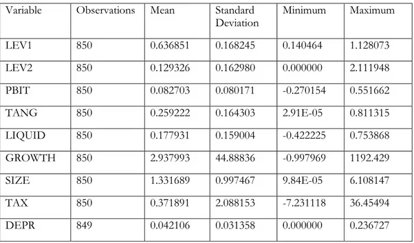
Basic features of the data are described using descriptive statistics. Simple summaries about the sample and the measures are provided. The following table shows the statistical information for 2005-2013 for both dependent variables and explanatory variables with regard to number of observations, mean, standard deviation and maximum and minimum values.

Table 4.1 Descriptive Statistics

Variable Observations Mean Standard

Deviation Minimum Maximum

LEV1 850 0.636851 0.168245 0.140464 1.128073 LEV2 850 0.129326 0.162980 0.000000 2.111948 PBIT 850 0.082703 0.080171 -0.270154 0.551662 TANG 850 0.259222 0.164303 2.91E-05 0.811315 LIQUID 850 0.177931 0.159004 -0.422225 0.753868 GROWTH 850 2.937993 44.88836 -0.997969 1192.429 SIZE 850 1.331689 0.997467 9.84E-05 6.108147 TAX 850 0.371891 2.088153 -7.231118 36.45494 DEPR 849 0.042106 0.031358 0.000000 0.236727 LEVERAGE 1

The table shows that LEV1 has a mean of 0.636851. This implies that 63.69% of the average firm total assets is finance by total debt. The companies in this sample are more leveraged compared to US companies with 29% as reported by Frank and Goyal (2009) and 35.5% of Norwegian companies as pointed out by Nilssen (2014).

LEVERAGE 2

The average LEV2 is 0.129326 indicating that the average company in the sample has a short debt level of 12.93%. Comparing this with the average LEV1, it implies that family firms in the OECD countries finance their assets using more long debt than short term debt. There is a slight difference in standard deviation for both dependent variables.

PROFITABILITY

The sample shows average profitability of 8.27% which is considerably higher than the mean of 6.55% for Norwegian firms reported by Nilssen (2014). Frank and Goyal (2009) found mean of 2% in their research on US companies. Song (2005) reported profitability

(18)

mean of 8% and a standard deviation of 0.28. The standard deviation is 0.08, this implies less variability compared to Norwegian firms and Swedish firms.

TANGIBILITY

This variable has a mean of 0.259222. It is less than average of 0.35 reported by Frank and Goyal (2009). In comparison, Nilssen (2014) got an average tangibility ratio of 0.395, which is higher than this sample. Furthermore she got a standard deviation of 0.30 which is significantly higher than the standard deviation of 0.164 from this sample.

LIQUIDITY

Liquidity has an average of 0.177931 and it can be interpreted as how much the average company is able to meet short term financial obligations. This ratio implies that for every 1 unit of current liabilities, a firm has an average of 0.178 units of current assets to cover short-term liabilities. This means that the family firms in OECD countries need to improve the level of current assets so that they can meet short term obligations. Nilssen (2014) achieved a liquidity ratio of 1.71 which indicates that Norwegian firms are better at meeting their short-term obligations.

GROWTH

This variable has an average of 2.937993 which indicates that the market expects future growth for the companies included in the sample. The mean of 1.84 was found by Nilssen (2014) for Norwegian firms, and the mean of 1.74 discovered by Frank and Goyal (2009) for US firms.

SIZE

The table shows the average size of 1.331689 with standard deviation of 0.997. Nilssen (2014) used logarithm of sales as a proxy for size, discovered mean of 14.3093 and standard deviation of 2.0045. This means that Norwegian firms have large differences in size between them compared to family firms in OECD countries.

DEBT-TAX SHIELD

This variable has a mean of 0.371891 and a standard deviation of 2.088. This indicates that 37.19% of taxable income from debt on family firms on OECD countries is reduced on average. This is achieved through claiming allowable deductions such as mortgage interest which reduce the family firms’ taxable income for a given year or defer income taxes into future years.

NON-DEBT TAX SHIELD

Non-debt tax shield has a mean of 0.042. This is slightly lower compared to mean of 0.049 obtained from Nilssen (2014). The same applies to the standard deviation from her research, which is 0.036 and about 0.005 higher than what was detected in this sample. The non-debt tax shield is achieved through claiming allowable deductions such as depreciation and amortization which reduce the family firms’ taxable income.

(19)

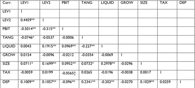
4.2 Correlation Analysis

The correlations between dependent variables and independent variables are presented in the table below.

Table 4.2 Correlation Matrix

In the correlation matrix, levels of significance at 1%, 5% and 10% are denoted by **, *, †respectively.

The table shows there is slightly strong correlation between leverage 1 and leverage 2 because both ratios are based on debt of the company. The correlation between most variables are relatively low. Profitability is significantly correlated with both leverage 1 and leverage 2. This agrees with the pecking-order theory that profitable firms prefer to finance internally. Asset tangibility is negatively correlated with both leverage ratios contrary to the trade-off theory. Firms’ liquidity is positively correlated to both leverage ratios but only significant with leverage 2. This also supports the idea of trade off theory on relationship between firms’ liquidity and leverage. Growth is positively correlated to leverage 1 and negatively correlated with leverage 2. Both leverage ratios are positively correlated with firms’ size. As firm gets larger, their debt also increases. Leverage 1 and leverage 2 are significant at 5% and 1% respectively. This agrees with trade-off theory. Leverage 1 is negatively correlated with tax shield while leverage 2 is positively correlated with debt-tax shield. The former is in contrast to what we expected while latter agrees with the trade-off theory. Non-debt tax shield is positively correlated to both leverage ratios contrary to what we expected. There is a significant positive relationship between non-debt tax shield and both leverage ratios.

4.3 Pooled Regression Model

Panel Least Squares analysis was conducted on the two models, on with leverage 1 as dependent variable and the other with leverage 2 as dependent variable with explanatory variables Profitability, Asset Tangibility, Growth, Size, Debt Tax Shield, Non-Debt Tax Shield and Liquidity.

Corr. LEV1 LEV2 PBIT TANG LIQUID GROW SIZE TAX DEP LEV1 1 LEV2 0.4459** 1 PBIT -0.5014** -0.315** 1 TANG -0.0746* -0.0537 -0.0006 1 LIQUID 0.0043 0.1915** 0.0969** -0.227** 1 GROW 0.0154 -0.0096 -0.0212 -0.0354 -0.0069 1 SIZE 0.0711* 0.1699** 0.0952** 0.0732* 0.2978** -0.0296 1 TAX -0.0059 0.0199 _-0.0565_†_0.0265 -0.0196 -0.0038 0.0017 1 DEP 0.1009** 0.1057** -0.096** 0.2341** -0.202** -0.0270 0.1029** 0.0259 1

(20)

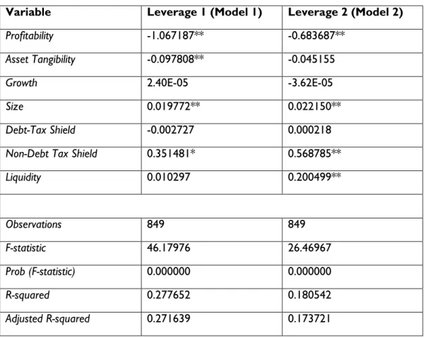
Table 4.3 Pooled Panel Least Squares Results

Variable Leverage 1 (Model 1) Leverage 2 (Model 2)

Profitability -1.067187** -0.683687**

Asset Tangibility -0.097808** -0.045155

Growth 2.40E-05 -3.62E-05

Size 0.019772** 0.022150**

Debt-Tax Shield -0.002727 0.000218

Non-Debt Tax Shield 0.351481* 0.568785**

Liquidity 0.010297 0.200499** Observations 849 849 F-statistic 46.17976 26.46967 Prob (F-statistic) 0.000000 0.000000 R-squared 0.277652 0.180542 Adjusted R-squared 0.271639 0.173721

Level of significance at 1%, 5% and 10% are denoted by **, *, † respectively

The two models are significant since the probabilities of statistics are less than 1%. F-statistic values for model 1 and model 2 are 46.17976 and 26.46967 respectively. The higher the F-value, the more of the total variability is accounted for in the model implying that model 1 has more explained variability than model 2. According to Koop (2013), R-squared measures the explanatory power of the model and indicates how the variance in the dependent variable can be explained by the independent variables. The results show that R-squared for model 1 is 0.277652 while that of model 2 is 0.180542, meaning that 27.76% of the variation in model 1 is explained by significant explanatory variables while only 18.05% of the variation in model 2 is explained by the significant independent variables.

Interpretation of Coefficients.

The results from the table above show that there are some differences in the magnitude of the coefficients for both models. While interpreting the coefficient of one variable, other variables are kept constant (ceteris paribus).

Profitability Model 1: Leverage 1

There is a negative relationship between leverage 1 and profitability. 1 unit increase in profitability, leverage 1 decreases by 1.067 units. The coefficient is significant at 1% significance level.

(21)

Model 2: Leverage 2

The regression results show that there is a negative relationship between leverage 2 and profitability. The results also indicate that when the profitability increases by 1 unit, leverage 2 decreases by 0.684 units. Like in the model 1, the coefficient is also significant at 1% level.

Asset Tangibility Model 1: Leverage 1

The regression indicates that there is a negative relationship between asset tangibility and leverage 1. 1 unit increase in the ratio of fixed assets to total assets leads to decrease in 0.098 units in leverage 1. Tangibility is significantly different from zero at 1% level of significance.

The results show that there is also a negative relationship between leverage 2 and tangibility. The coefficient is not significant at 1%, 5% and 10% significance level.

Growth

There is a slight positive relationship between growth and leverage 1. Growth is not significantly different from zero at 1%, 5% or 10% significance level.

Unlike the model 1, the results show there is a slight negative relationship between leverage 2 and growth. Also in this model, growth is not significant at 1%, 5% or 10% significance level.

Size

A positive relationship was found to exist between size and leverage 1 according to the results in the table above. When size increases by 1 unit, leverage 1 also increases by 0.0198 units. The coefficient is significant at 1% level of significance.

The regression results show that there is also a positive relationship between size and leverage 2. 1 unit increase in size causes leverage 2 to increase by 0.022 units and the coefficient is significantly different from zero at 1% level of significance.

Debt-Tax Shield Model 1: Leverage 1

There is a negative relationship between debt-tax shield and leverage 1. The coefficient is not significantly different from zero at 1%, 5% or 10% significance level.

A positive relationship exists between leverage 2 and debt-tax shield. Debt-tax shield is not significant at 1%, 5% or 10% significance level.

(22)

Non-Debt Tax Shield Model 1: Leverage 1

The regression results show that there is a positive relationship between non-debt tax shield and leverage 1. 1 unit increase in non-debt tax shield will result into a 0.351 increase in units of leverage. The coefficient is significantly different from zero at 5% level of significance.

There is a positive relationship between leverage 2 and non-debt tax shield. When non-debt tax shield increases by 1 unit, leverage 2 increases by 0.569 units. Non-debt tax shield is significant at 1% level.

Liquidity Model 1: Leverage 1

The results obtained a positive relationship between liquidity and leverage 1. The coefficient in not significant at 1%, 5% or 10% significance level.

A positive relationship exists between leverage 2 and liquidity. The results indicate that 1 unit increase in liquidity will cause the leverage 2 to increase by 0.2005 units, while the coefficient is significantly different from zero at 1% level.

4.4 Panel Regression Model with Random Effects

The analysis explores how firm-specific factors affect firms’ level of leverage by using panel regression model with random effects. Interpretation of the coefficients in a random effects model is different from the panel least squares as the coefficients include both within-entity and the between-entity effects, Nilssen (2014). When interpreting the results, the coefficient will represent the average marginal effect of explanatory variables over dependent variable, when explanatory variable changes across time and between firms by 1 unit. It means that the random effects regression model does not only predict change over time but also it takes into account the difference between units.

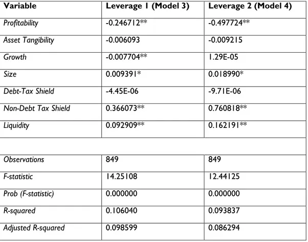
Model 3 and model 4 are both significant since the probability of F-statistics are less than 1%. F-statistic values for model 3 and model 4 are 14.25108 and 12.44125 respectively. The higher the F-value, the more of the total variability is accounted for in the model implying that model 3 has more explained variability than model 4. R-squared measures the explanatory power of the model and indicates how the variance in the dependent variable can be explained by the independent variables. The results show that R-squared for model 3 is 0.106040 while that of model 4 is 0.093837, meaning that 10.60% of the variation in model 3 is explained by significant independent variables while only 9.38% of the variation in model 4 is explained by the significant explanatory variables. This shows that there is a small difference between the models and the ability of the explanatory variables to explain variation across firms. Conclusively the explanatory variables can explain 1.22% more of the variation in model 3 than that of model 4.

(23)

Table 4.4 Random Effects Regression Model Results

Variable Leverage 1 (Model 3) Leverage 2 (Model 4)

Profitability -0.246712** -0.497724**

Asset Tangibility -0.006093 -0.009215

Growth -0.007704** 1.29E-05

Size 0.009391* 0.018990*

Debt-Tax Shield -4.45E-06 -9.71E-06

Non-Debt Tax Shield 0.366073** 0.760818**

Liquidity 0.092909** 0.162191** Observations 849 849 F-statistic 14.25108 12.44125 Prob (F-statistic) 0.000000 0.000000 R-squared 0.106040 0.093837 Adjusted R-squared 0.098599 0.086294

Level of significance at 1%, 5% and 10% are denoted by **, *, † respectively

The interpretation of coefficients of the random effects regression model for model 3 and model 4 is discussed in the analysis section accompanied by firm-specific effect on capital structure.

(24)

5 ANALYSIS

This chapter aims to actualise the purpose and answer the research questions through the combina-tion of hypotheses and empirical findings.

In this section, the results from the coefficients obtained from the random effects regression models are analysed and discussed in order to determine the effect of the chosen firm-specific factors on capital structure.

5.1 Profitability

The profitability-variable is significant at 1% for both leverage 1 and leverage 2 as dependent variables in model 3 and model 4 respectively. For both models, profitability is negative indicating that family firms with higher returns tend to have lower levels of leverage. The results suggest that 1 unit increase in profitability leads to 0.247 decrease in units of leverage 1. For model 4, when profitability increases by 1 unit, leverage 2 decreases by 0.498 units.

The two capital structure theories provide different views on the effect of profitability on leverage. The pecking-order theory argues that there is an inverse relationship between leverage and profitability. Our results are consistent with the pecking-order theory. This implies that more profitable family firms use less leverage because they use retained earnings as funding instead of external debt. In contrast, the trade-off theory assumes that profitable firms will shield their profits from tax, hence borrow more than less profitable firms. The fact that both models suggest a negative relationship between profitability and leverage are consistent with the results from Rajan and Zingales(1995), Frank and Goyal (2004) and Nilssen (2014). Positive relationship between profitability and leverage is rarely supported by recent empirical studies.

5.2 Asset Tangibility

For both models, tangibility is not significantly from zero at 1%, 5% or 10% significance level. The results show that tangibility has a negative relationship with leverage for both models.

These results are in contrast with both theories which predicts a positive relationship between tangibility and leverage. The pecking-order theory suggests that information asymmetry is lower for firms with more tangible assets, resulting in more debt. However, the results are in consistent with Harris and Raviv(1991) who argued that the pecking-order theory suggests a negative relationship between tangibility and debt. Family firms with few tangible assets have greater asymmetry problems, hence the coefficient should not be significantly different from zero. The trade-off theory also predict a positive relationship between tangibility and debt simply because higher degree of asset tangibility leads to lower bankruptcy costs.

Fixed assets may be used as collateral hence we expected a positive relationship between tangibility and debt, but the study found different results. Maybe family firms in OECD countries do not prefer to use fixed assets as collateral to borrow more. However, Alves and Ferreira(2011) concluded that asset tangibility decreases with short-term debt but increases with long-term debt.

(25)

5.3 Growth

Growth has a negative relationship with leverage 1 and it is significantly different from zero at 1% significance level. 1 unit increase in growth will result into a 0.0077 decrease in units of leverage 1 for model 3. However the results show that growth has a slight positive relationship with leverage 2 and its coefficient is not significant for model 4.

The cost of bankruptcy and financial distress are considerably higher for a company with a lot of growth opportunities, Titman & Wessels (1988). Model 3 is consistent with trade-off theory which assumes a negative relationship between growth and leverage because firms with prospects of growth are likely to have lower earnings before tax, thus they can’t take advantage of the interest tax shield which are associated with high leverage. On top of that, growing firms are likely to appreciate financial flexibility, hence preferably debt ratio.

Since model 4 is not statistically significant, there is no evidence that growth affects leverage 2. The results for model 3 are contrary with pecking-order theory which suggests that firms would need external funds to finance investment projects as they are unable to finance all investment opportunities through their internal sources (Smith, 2010). Family firms in OECD countries with prospects of growth seem to have lower earnings before tax, hence they are likely to appreciate financial flexibility. Generally, the results for model 3 are in consistent with other empirical studies including Rajan & Zingales (1995), Shah & Khan (2007) and Frank & Goyal (2007) who achieved a negative effect of growth on leverage.

5.4 Size

The size-variable is significantly different from zero at 5% significance level for both models. The results indicate a positive relationship between leverage and size for model 3 and model 4. When size increases by 1 unit, leverage 1 increases by 0.0093 units for model 3 while leverage 2 increases by 0.019 units. Both models are in consistent with trade-off theory which argues that larger firms are usually more diversified and have relative low bankruptcy risks (Luambano, 2012). This enhances the capacity of family firms in OECD countries to access short term debt finance and hence the positive relationship. The pecking-order theory justifies the expectation of positive relationship existing between leverage and size with a lower degree of information asymmetry will give companies better opportunities and conditions to gain access to credit. This is in contrast with pecking-order theory that suggests a negative relationship exists between size and leverage. Rajan and Zingales (1995) argued that larger firms have less information asymmetry than smaller firms because they disclose more information to outsiders than smaller firms hence they are expected to have more equity than debt due to low asymmetrical information costs advantage they have.

5.5 Debt -Tax Shield

The results show that there is a very slight negative relationship between debt-tax shield and leverage for both models. However, the variable is not significantly different from at 1%, 5% or 10% significance level. Furthermore the results are in contrast to the trade-off theory which predicts a positive relationship between debt-tax shield and leverage. The

(26)

capital structure contrary to what we expected. Firms hold debt levels which maximize tax benefits of debt but minimize bankruptcy risks, hence debt level increases as long as debt benefits outweigh bankruptcy risks otherwise it falls (Luambano, 2012).

5.6 Non-Debt Tax Shield

Non-debt tax shield is significantly different from zero at 1% significance level for model 3 and model 4. The results show that the variable has a positive relationship with leverage for both models. When non-debt tax shield increases by 1 unit, leverage 1 increases by 0.366 units and leverage 2 increases by 0.761 units of leverage 2 respectively. The results are in contrast with the trade-off theory which predicts a negative relationship exists between non-debt tax shield and leverage. However, the results are in consistent with Delcoure (2007) who found non-debt tax shield positively affect debt. Family firms in OECD countries take the advantage by claiming allowable deductions such as amortization and depreciation that reduce the taxable income. As a result this will increase non-debt tax shield, hence preferably high debt ratio.

5.7 Liquidity

Liquidity is significantly different from zero at 1% significance level for model 3 and model 4. Both models indicate a positive relationship between liquidity and leverage so that 1 unit increase in liquidity will result into a 0.093 increase in units of leverage 1 and 0.162 increase in units of leverage 2 respectively. The results are consistent with the trade-off theory which predicts a positive relationship between leverage and liquidity. Higher liquidity signify that the firm is financially health and it has low bankruptcy risks. Smith (2010) argued that an increase in firm’s liquidity leads to high debt level as firm’s capacity to borrow rises. The family firms in OECD countries with high liquidity are financially health and are likely to have low bankruptcy risks hence favour them to borrow more. However, the results are in contrast with pecking-order theory which argues that firms prefer internal to external financing, hence they would create liquid reserves from retained earnings. When the liquid assets are sufficient in financing a firms’ investments, the firm would have no incentive to raise fund from external source (Nilssen, 2014).

Analysis above tries to answer the three research questions discussed in chapter 1 which are:

1. What are the determinants of determinants of capital structure? 2. How do these determinants affect the capital structure of family?

3. Do the capital structure theories predict similar relationship between capital structure and its determinants for family firms?

(27)

6 DISCUSSION

This chapter aims to present discussion on the results of the study, limitations and further research.

6.1 Conclusions

Number of theories explaining the role of capital structure in a firm have been developed since Modigliani and Miller (1958) proposed the irrelevance of capital structure for a firm value. Pecking-order theory and trade theory are the most prominent theories in explaining the capital structure. The pecking-order theory stresses that firms prefer internal to external funding and debt over equity because of the information asymmetry while the trade-off theory explains that the choice of capital structure is a result of trade-off between benefits and costs of debt. Number of studies have been conducted on this topic for different determinants and different regions, focusing on firms in general without categorizing family firms and non-family firms. The purpose of this study was trying to fill the gap in the existing literature focusing on family firms and providing some useful information about the determinants of capital structure in OECD countries.

The overall aim of this study was to identify the factors which influence capital structure and how they affect the family firms financing decisions in the OECD countries. Furthermore this study aimed at testing how the identified determinants of capital structure are affecting OECD family firms. Also this research wanted to verify whether the general capital structure theories predict similar relationships between the capital structure and its determinants in OECD family firms.

Based on the previous empirical studies, six firm specific determinants of capital structure were identified including; profitability, asset tangibility, growth, size, liquidity and tax shields. Profitability and leverage were given special attention in the pecking-order theory while other four variables were mainly linked to trade-off theory. The study comprises of 95 firms from nine OECD countries over a time period of 9 years from 2005-2013.

The data was collected from Amadeus database and firms had to have reported annual financial data for the entire period. Dataset included 95 firms for 9 years representing 850 complete observations for firm characteristics.

Preliminary analysis was conducted through descriptive statistics and correlation analysis. Pooled panel regression model followed by random effects regression model were performed. The regression results were analysed, then based on the results an attempt was made to answer the research questions of the study.

The findings showed that the independent variables are able to explain 10.60% of the variance for model 3 and 9.38% for model 4. The significant variables for model 3 were profitability, growth, size, non-debt tax shield and liquidity while for model 4 only profitability, size, non-debt tax shield and liquidity were significant. Profitability, tangibility, growth and debt-tax shield had a negative relationship with leverage 1, while other three variables found to have a positive relationship with leverage 1 for model 3. Leverage 2 had a positive relationship with growth, size, non-debt tax shield and liquidity. Profitability, tangibility and debt-tax shield had a negative relationship with leverage 2 for model 4. The results showed that both pecking-order theory and trade-off theory explain the capital structure of family firms in OECD countries for model 3 and model 4.

(28)

6.2 Limitations

In this study, only six firm-specific characteristics of capital structure were identified and analysed. There is large set of possible variables that may influence the capital structure decisions. It was difficult for us to identify all of them, for practical reasons some of them are difficult to measure such as risky and management style.

We could not find a reliable database for family firms, we decided used global family index of St. Gallen University in Switzerland to find family firms in OECD countries.

We decided to reduce the sample size to 95 family firms from 2005 -2013 due to unavailability of financial data for many firms in the Amadeus database.

6.3 Further Research

From an international point of view, there is need to do more research in order to verify if countries regulatory aspect and national or cultural aspect could affect the capital structure of family firms. Another interesting area of research could be could possibly be the integration of the socio-emotional wealth dimension with law and finance approach, taking into account the level of protection of investors and the rights of shareholders and creditors to develop a comprehensive model for financial decisions for family firms.

Furthermore, there has been a number of studies on the capital structure for family firms in developed countries and the case of family firms in developing countries has been abandoned. There is need to do a comparison of capital structure for family firms in developed and developing economies as well as verify if there are any similarities or differences between them and identifying the loop holes and possible solutions.

Determinants of Capital Structure in Family Firms