Mid Sweden University Department of Social Sciences
Business Administration D Master Thesis
Fachhochschule Aachen Fachbereich Wirtschaftswissenschaften
Europäischer Studiengang Wirtschaft Diplomarbeit
T
HE
I
MPACT OF
W
ORKING
C
APITAL
M
ANAGEMENT
ON
C
ASH
H
OLDINGS
–
A Quantitative Study of Swedish Manufacturing SMEs
Author: Maxime Abel
Place of Birth: Frankenthal, Germany
1st Examiner: Prof. Håkan Boter (Mid Sweden University)
2nd Examiner: Prof. Dr. Jürgen Stephan (Fachhochschule Aachen)
Tutor: Dr. Darush Yazdanfar
Term: Summer 2008
Abstract
This study examines the impact of working capital management on cash holdings of small and medium-sized manufacturing enterprises in Sweden. The aim of this work is to theoretically derive significant factors related to working capital management which have an influence on the cash level of SMEs and test these in a large sample of Swedish manufacturing SMEs. The theoretical framework for this study consists of a treatise of motives for holding cash, working capital management and cash level. From these theoretical findings, two hypotheses are deduced:
• H1: Cash holdings are negatively related to the presence of cash substitutes
• H2: Cash holdings are positively related to working capital management efficiency
The quantitative investigation consists of the statistical analysis – namely comparison of means and correlation analysis – of key figures which are calculated from the financial statements of a large sample of firms. The dataset contains 13,287 Swedish manufacturing SMEs of the legal form ‘Aktiebolag’. Both hypotheses are confirmed by the results. Empirical evidence is presented which substantiates the supposition that the presence of cash substitutes – namely inventory and accounts receivable – entails lower cash holdings. Furthermore, it is confirmed that working capital management efficiency – measured by the cash conversion cycle – is positively related to cash level. The discussion of the empirical findings pays regard to the different subordinate components of both cash substitutes and working capital management efficiency. Implications of the detected findings are highlighted with respect to their potential utility for the achievement and maintenance of a firm’s target cash level.
Table of contents
1 Introduction ...1
1.1 Importance of the topic... 1
1.1.1 Significance of SMEs ... 1
1.1.2 Financial constraints of SMEs... 3
1.2 Introduction to this study ... 4
1.2.1 Problem formulation ... 4
1.2.2 Delimitation ... 5
1.2.3 Objectives ... 5
1.2.4 Disposition... 6
2 Theoretical background...7
2.1 Definition of key terms and concepts... 7
2.1.1 SME... 7
2.1.2 Cash ... 8
2.1.3 Working capital... 8
2.1.4 Marketable securities ... 8
2.1.5 Days sales outstanding ... 9
2.1.6 Days sales of inventory ... 9
2.1.7 Days payable outstanding... 9
2.1.8 Cash conversion cycle ... 9
2.2 Keynesian motives for holding cash ... 9
2.2.1 The transactions-motive... 10
2.2.2 The precautionary-motive ... 10
2.2.3 The speculative-motive ... 10
2.2.4 Strength of the Keynesian motives ... 11
2.2.5 Relevance of the Keynesian motives... 11
2.3 Working capital management... 12
2.3.1 Inventory management ... 13
2.3.2 Cash management... 16
2.3.3 Credit management... 19
2.3.4 Working capital policy ... 21
2.4 Cash level... 25
2.4.1 Advantages & disadvantages of cash holding ... 26
2.4.2 The determinants of cash level ... 26
2.4.3 Cash level in SMEs ... 30
2.5 Hypotheses ... 31 2.5.1 Hypothesis 1 ... 31 2.5.2 Hypothesis 2 ... 32 3 Methodology ...34 3.1 Research aim ... 34 3.2 Research design... 34 3.3 Sampling ... 35 3.3.1 Choice of sample ... 35 3.3.2 Sampling procedure ... 35 3.4 Variables... 36 3.5 Statistical methods... 37 3.6 Research quality... 38 3.7 Strengths... 39 3.8 Limitations ... 40
4 Presentation of empirical data ...41 4.1 Description of dataset... 41 4.2 Descriptive statistics... 44 4.3 Univariate results ... 45 4.4 Bivariate results... 47 5 Analysis of results ...49 5.1 Hypothesis results ... 49 5.1.1 Hypothesis 1 ... 49 5.1.2 Hypothesis 2 ... 49
5.1.3 Recapitulation of hypothesis results ... 50
5.2 Discussion of results ... 51
5.2.1 Significance of hypothesis results... 51
5.2.2 Causality... 54
5.2.3 Net working capital and cash conversion cycle ... 56
5.2.4 Accounts receivable ... 56
5.3 Implications... 57
5.3.1 Target cash level... 57
5.3.2 The impact of cash conversion ... 58
5.3.3 The strength of substitutes for cash... 59
5.3.4 Conclusion ... 61
6 Concluding discussion...62
6.1 Recapitulation of the work... 62
6.2 Achievement of objectives ... 63
6.3 Recommendations for future research ... 64
Bibliography ...i
Appendices ...vii
Appendix A: Calculation of variables... vii
Appendix B: Sampling procedure ... viii
Appendix C: Sample statistics... ix
Declaration of honour ...xii
List of tables
Table 1: Detailed figures on SMEs and large enterprises in Sweden ... 3
Table 2: Definition of Medium-sized, Small and Microenterprises ... 7
Table 3: Different working capital policies and impacts on return on assets (setting A) .. 22
Table 4: Different working capital policies and impacts on return on assets (setting B) .. 23
Table 5: Factors that are positively related to cash level... 28
Table 6: Factors that are negatively related to cash level ... 29
Table 7: Descriptive statistics of relevant sample features... 42
Table 8: Descriptive statistics of variables... 44
Table 9: Comparison of means... 45
Table 10: Correlation table (* = significant at the 0.01 level)... 47
Table 11: Results of hypothesis testing ... 50
List of figures
Figure 1: Repartition of SMEs (grey) and large enterprises (black) in the EU-27 ... 1Figure 2: Repartition of SMEs (grey) and large enterprises (black) in Sweden ... 2
Figure 3: Graphic determination of the optimal size of inventory (draft)... 15
Figure 4: Graphic determination of the optimal cash level (draft)... 18
Figure 5: Graphic determination of the optimal credit policy (draft)... 20
Figure 6: Graphic determination of the optimal level of current assets (draft)... 24
Figure 7: Graphic determination of the optimal level of current assets with decreased carrying costs (draft) ... 25
Figure 8: Histogram featuring number of employees ... 42
Figure 9: Histogram featuring turnover (k SEK) ... 43
Figure 10: Repartition of micro, small and medium-sized enterprises among the sample firms... 43
List of abbreviations
DPO: Days Payable Outstanding
DSI: Days Sales of Inventory
DSO: Days Sales Outstanding
EBIT: Earnings Before Interests and Taxes
EOQ: Economic Order Quantity
EU: European Union
EUR: Euro
OECD: Organisation for Economic Co-operation and Development
SEK: Swedish Krona
SME: Small and Medium-sized Enterprises
SNI: Svensk Näringsgrensindelning (=Swedish Standard Industrial Classification)
1 Introduction
SMEs being a “key source of dynamism, innovation and flexibility in advanced industrialised countries, as well as in emerging and developing
economies” 1 , their well-being and continuity are crucial to the
macroeconomic development of any country around the globe. The financing problems that SMEs frequently have to face2 reflect the need to study the financial conditions of this enormous and significant3 size class of enterprises. Hence, this introductory section aims at further revealing the significance of this work’s topic and afterwards introducing the basic conception of this study.
1.1 Importance of the topic
In the following, the high significance of the topic is being illustrated. For this purpose the significance of SMEs for the European as well as the Swedish economy is displayed. Afterwards, current financial problems that SMEs face are presented.
1.1.1
Significance of SMEs
According to data from 2004 collected by the ‘Statistical Office of the European Communities’ which analyzes structural business statistics from the EU-27 countries, SMEs constitute 99.8% of the total amount of enterprises in the non-financial business sector. 56.9% of the value added is generated by SMEs and they account for 66.7% of the European workforce employment.4
Share in total amount of enterprises 99,8% 0,2% Share in workforce 56,9% 43,1%
Share in value added
66,7% 33,3%
Figure 1: Repartition of SMEs (grey) and large enterprises (black) in the EU-27
1 OECD (2006), “The SME Financing Gap (Volume I) – Theory and Evidence”, p. 9 2 cp. section 1.1.2
3 cp. section 1.1.1 4 cp.
http://epp.eurostat.ec.europa.eu/portal/page?_pageid=2293,59872848,2293_68195655&_dad=port al&_schema=PORTAL#smes1
Besides their quantitative prevalence, SMEs also have a significant qualitative input to the European economy regarding innovative development. A 1996 survey conducted by the European Commission points out that 51% of the European SMEs can be considered as innovative, i.e. “enterprises that introduced technologically new or improved products, processes or services during the reference period”.1
This figure needs to be considered under the assumption that “[t]he larger an enterprise, the more likely it is to capitalize on innovation”2, meaning
that larger firms are more likely to be innovative than small ones. Furthermore, SMEs have an immense impact on the global employment development. According to a 2000 OECD report, “SMEs will be […] the major source of jobs” “surpassing larger firms in net job creation”.3
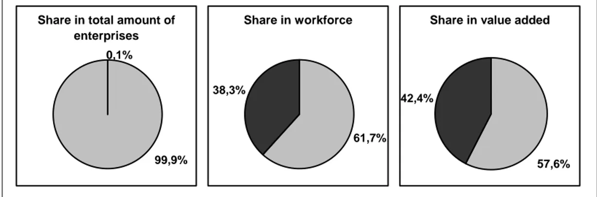
In Sweden, there is a significant number of SMEs. According to structural business statistics from the ‘Official Statistics of Sweden’ using data from the year 20054, SMEs make up for 99.9% of the Swedish enterprises and
employ 61.7% of the Swedish workforce, i.e. 1,398,994 people. 57.6% of the Swedish value added is produced by SMEs.
Share in total amount of enterprises 99,9% 0,1% Share in workforce 61,7% 38,3%
Share in value added
57,6% 42,4%
Figure 2: Repartition of SMEs (grey) and large enterprises (black) in Sweden
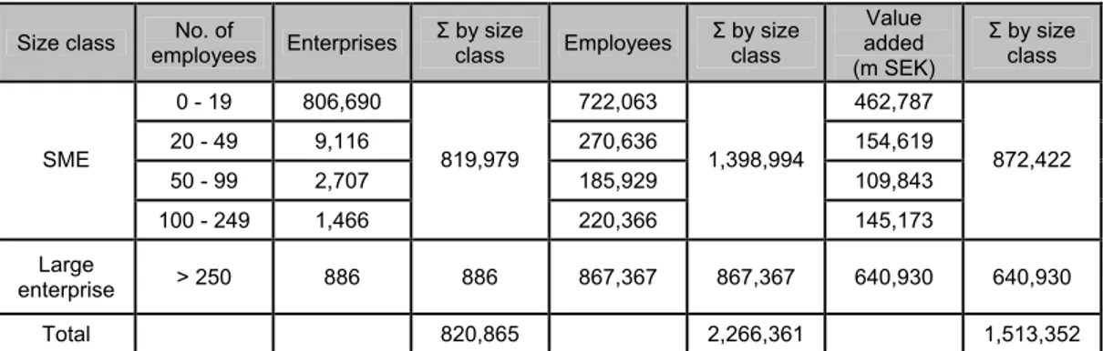
The following table recapitulates the absolute numbers5 which constitute the basis for the above illustrated repartition between SMEs and large enterprises in Sweden. These figures should allow for a more detailed insight into the Swedish structural business statistics.
1 European Communities (2002), “SMEs in Europe – Competitiveness, innovation and the
knowledge-driven society”, p. 30
2 The Gallup Organization (2007), “Observatory of European SMEs – Summary”, p. 2
3 OECD (2000), “OECD Small and Medium Enterprise Outlook – Enterprise, Industry and Services”,
p. 9
4 cp. http://www.ssd.scb.se/databaser/makro/produkt.asp?produktid=nv0109&lang=2 5 cp. ibid.
Size class employees No. of Enterprises Σ by size class Employees Σ by size class Value added (m SEK) Σ by size class 0 - 19 806,690 722,063 462,787 20 - 49 9,116 270,636 154,619 50 - 99 2,707 185,929 109,843 SME 100 - 249 1,466 819,979 220,366 1,398,994 145,173 872,422 Large enterprise > 250 886 886 867,367 867,367 640,930 640,930 Total 820,865 2,266,361 1,513,352
Table 1: Detailed figures on SMEs and large enterprises in Sweden
Seemingly, SMEs constitute an important element of both the European and the Swedish economy. They employ approximately two thirds of the workforce and contribute considerably to the value added. Nevertheless, SMEs exhibit significant exit rates. According to an OECD report, about 20% of newly created enterprises do not survive their first year.1 It should be noted that the data refer to the total amount of exits. It therefore contains deliberate as well as involuntary endings. In Sweden, the total amount of bankruptcies, i.e. involuntary exits, has decreased since 2003.2 In 2006, the ‘Official Statistics of Sweden’ totalled 6,160 enterprise
bankruptcies. 3 In the same year, the number of newly registered
businesses was 59,6134, accounting for an entry rate of roughly 7%. Taking into consideration the significant prevalence of SMEs on the Swedish market, the share of large companies in these figures can be assumed to be negligible.
1.1.2
Financial constraints of SMEs
Obviously, SMEs are of vital importance to the Swedish economy and the above mentioned data indicate that the entry rate significantly exceeds the exit rate, evidence which is supported by the findings of the OECD.5 Clearly, this leads to a strong increase of Swedish SMEs in quantity and therefore significance as well. Nevertheless, the number of liquidations is still considerable and displays the importance of studying SMEs with regard to financial aspects. This is also supported by the factors which lead to SME bankruptcy. Many authors have studied these reasons for SME failure.6 The results indicate that one issue is widespread among the
1 cp. OECD (2005), “SME and Entrepreneurship Outlook”, p. 22
2 cp. Statistics Sweden (2008), “Statistical Yearbook of Sweden 2008”, p. 188 3 cp. ibid.
4 cp. ibid. at p. 190 5 cp. OECD (2005), p. 23
6 cp. Peterson, R.; Kozmetsky, G.; Ridgway, N. (1983), “Perceived Causes of Small Business
Failure: A Research Note”, American Journal of Small Business, Vol. 8, Issue 1, pp. 15-19; cp. Hall, G. (1992), “Reasons for Insolvency Amongst Small Firms – A Review and Fresh Evidence”, Small Business Economics, Vol. 4, Issue 3, pp. 237-250
factors which lead to SME bankruptcy: Lack of capital.1 OECD analysts
agree that access to finance is one of the most significant hindrances for the establishment and development of SMEs.2 Among the most important
start-up difficulties detected within a 2005 survey published by the ‘Statistical Office of the European Communities’ are ‘Financing’, ‘Outstanding invoices’ and ‘Finding suppliers’3, all of which are closely
related to working capital management. According to a 2006 survey published by the European Commission, about every fifth European SME has encountered difficulties related to limited access to finance. 4
Furthermore 44% of the respondents claimed that this constraint had increased during the two years preceding the survey.5 The OECD refers to
this problem as the ‘SME financing gap’ and has devoted a global conference to this issue.6 According to the conference’s report, SMEs
display “significant gaps in information and skills needed to access external finance”.7 Although financing gaps are more current in emerging
than in developed markets, they are nevertheless existent in OECD countries, especially regarding innovative SMEs.8
Seemingly, SMEs are challenged by several financial constraints which can partly be connected to working capital management. Therefore, the topic of working capital management is of great importance for SMEs in order to avoid financial bottlenecks since the availability of external funds can be rather low.9
1.2 Introduction to this study
The following section aims at giving a precise impression of this work’s conception. In order to achieve this, the exact problem is formulated and delimited. Thereafter, the objectives are presented and lastly, the disposition section displays the structure of the work.
1.2.1 Problem
formulation
Despite the immense and increasing importance of SMEs for the European and Swedish economy and their prevailing financial problems described in the previous section, not much financial management theory
1 cp. Peterson, R. et al. (1983), p. 18; cp. Hall, G. (1992), p. 245
2 cp. OECD (2004a), “OECD Compendium II on SME and Entrepreneurship Related Activities”, p.
75
3 cp. Schrör, H. (2006), “The profile of the successful entrepreneur – Results of the survey ‘Factors
of Business Success’”, p. 8
4 cp. The Gallup Organization (2007), p. 8 5 cp. ibid. at p. 9
6 “Better Financing for Entrepreneurship and SME Growth” (Brasilia, 27th – 30th March 2006) 7 OECD (2006), p. 13
8 cp. ibid. 9 cp. ibid. at p. 9
exists with special regards to SMEs. Most theory in this field of study is related to corporate financial management. This also applies to empirical studies which are mainly conducted in large enterprises.1 Obviously,
financial management in SMEs and large enterprises bear strong similarities. However, there is a significant disparity which substantiates the study of financial management in SMEs. Since smaller firms experience difficulties in accessing external finance, they rely more strongly on internally generated funds than large firms.2 Working capital
management thus plays an important role in the financing of SMEs. This assumption is confirmed by the fact that working capital related problems are cited among the most significant reasons for the failure of SMEs. As working capital management is related to short-term financial planning and cash level or liquidity in general represents a significant indicator for short-term performance, the impact of the first on the latter – which constitutes this study’s topic – should be of crucial importance.
1.2.2 Delimitation
This work studies the impact of working capital management on cash holdings in Swedish manufacturing SMEs. In this respect, a delimitation has been undertaken in that only Swedish manufacturing firms of a certain size are included in the dataset. The theoretical section presents aspects which are not strictly delimitated to a certain size class, country or industry. However, a focus on the SME size class is given by discussing the relevance of several aspects for SMEs.
1.2.3 Objectives
The objectives of the paper are being presented in the following part. First, the purpose of the study is discussed. Afterwards, the targeted readership is defined and formulated.
The purpose of this study is to analyze the impact of working capital management on the level of cash held by Swedish manufacturing SMEs. The aim of the theoretical section is to present a detailed discussion of the concepts and theories which constitute the basis for the empirical analysis. This theoretical knowledge is condensed in the hypotheses which are subsequently tested in the context of Swedish manufacturing SMEs. The aim of the empirical section is to find statistical evidence which is
1 cp. section 2.4.2
2 cp. Weston, J. & Copeland, T. (1986), “Managerial finance", Eighth Edition, Hinsdale: The Dryden
significant enough to confirm or reject the hypotheses and afterwards discuss the results so as to add new aspects to the existing research.
The targeted readership is composed of practitioners as well as academics. Decision-makers from SMEs, financial service providers as well as policy makers should be interested in the results as they should lead to an enhanced understanding of cash level and its determinants in SMEs, not only of the manufacturing sector. Academics could benefit from this work in that they should discover an alternative theoretic approach to explaining cash holding decisions in SMEs.
1.2.4 Disposition
The structure of this work is basically divided into a theoretical, a methodological and an empirical section. The theoretical framework consists of a treatise of motives for holding cash which have been formulated by John Maynard Keynes, a presentation of working capital management and all of its components and a discussion of cash level including determinants which impact cash holdings. On the basis of the theoretical treatise, two hypotheses are formulated. The methodology section describes and justifies the methodological approach which has been used in order to test the hypotheses. Subsequently, the empirical part first describes and then analyzes the results which have been extracted from the dataset. Finally, after having recapitulated the thesis, the concluding discussion deals with the issue whether the aims and purposes of this work have been fulfilled. On this basis, recommendations for future research are made.
2 Theoretical
background
In the following, the theoretical background will be presented. It consists of five parts. The first part aims at defining key terms and concepts. The motives for holding cash are dealt with in the second section. The third part is dedicated to working capital management. The aspect of cash level is discussed in the fourth section and finally, the fifth part acts as a summary of the whole theoretical background by formulating the hypotheses which are based on the theoretical findings and which will be tested in the empirical section.
2.1 Definition of key terms and concepts
This section provides a clear definition of terms and concepts that are used in this work. It aims at avoiding misunderstandings and should help the reader understand the basic conceptions on which this paper is based.
2.1.1 SME
There is no unique definition of SME. In 2000, the ‘Official Statistics of Sweden’ defined SMEs as “enterprises with less than 50 employees”.1 The German ‘Institut für Mittelstandsforschung’ defines SMEs as companies with less than 500 employees or a turnover of less than 50 m EUR.2 By reason of the discrepancy of its member states’ definitions, the European Union has provided a standardized definition which Sweden and the other EU member states have subsequently adopted.3 The official EU definition4 which is used in this work can be summarized by the following table:
Enterprise size Employees No. of Turnover (m EUR) [m SEK] Balance sheet (m EUR) [m SEK] Medium-sized enterprise < 250 and [~472] ≤ 50 or [~406] ≤ 43 Small enterprise < 50 and [~94] ≤ 10 or [~94] ≤ 10 Microenterprise < 10 and [~19] ≤ 2 or [~19] ≤ 2
Table 2: Definition of Medium-sized, Small and Microenterprises
1 Statistics Sweden (2000), “The environment industry in Sweden 2000 – Employment and
economic data for enterprises primarily producing environmental goods and services”, p. 49
2 cp. http://www.ifm-bonn.org/index.php?id=89
3 cp. OECD (2004b), “SME Statistics: Towards a More Systematic Statistical Measurement of SME
Behaviour”, p. 147
4 cp. The Commission of the European Communities (2003), “Commission Recommendation of 6
May 2003 concerning the definition of micro, small and medium-sized enterprises”, Official Journal of the European Union L124, Vol. 46, pp. 36-41, p. 39
2.1.2 Cash
The term cash refers to the “most liquid of assets”.1 According to Weston & Copeland cash includes “demand deposits and money market accounts as well as currency holdings”.2 It should be noted that in this work, cash shall be defined as cash plus cash equivalents, i.e. highly liquid short-term investments such as marketable securities. This assumption is due to the fact that this broad definition of cash forms the basis for the subsequent theory. Additionally, the characteristics of the empirical data for this study do not allow for a differentiation between cash and cash equivalents. Obviously, the broad definition does not apply to the section on the cash management model3 which explicitly requires a strict distinction between cash and marketable securities.
2.1.3 Working
capital
In corporate annual reports, working capital is mostly defined as follows: Current assets minus current liabilities.4 Hence, it “represents the firm’s
investment in cash, marketable securities, accounts receivable, and inventories less the current liabilities used to finance the current assets”.5
Some authors may refer to working capital as the sum of current assets and current liabilities and define the difference (current assets minus current liabilities) as ‘net working capital’.6 However, in the following, the
term working capital will be used as determined in the first definition. The expression ‘Net Working Capital’ will be used as a variable in the empirical part to designate the ratio of working capital less cash to assets.
2.1.4 Marketable
securities
Weston & Copeland refer to marketable securities as a “portfolio of highly liquid, near-cash assets which serves as a backup to the cash account”.7 There are several types of marketable securities, such as ‘Treasury securities’, ‘Repurchase agreements’, ‘Agency securities’ or ‘Commercial papers’.8 Marketable securities with a maturity of less than three months are referred to as ‘cash equivalents’ on the balance sheet, those with a longer maturity as ‘short-term investments’.9
1 Van Horne, J. (1995), “Financial management and policy”, Tenth Edition, Englewood Cliffs:
Prentice Hall, p. 359
2 Weston, J. & Copeland, T. (1986), p. 289 3 cp. section 2.3.2.1
4 cp. Weston, J. & Copeland, T. (1986), p. 277 5 ibid.
6 cp. Brealey, R. & Myers, S. (2003), “Principles of Corporate Finance”, Seventh Edition, New York:
McGraw-Hill, p. 851
7 Weston, J. & Copeland, T. (1986), p. 289 8 cp. Van Horne, J. (1995), pp. 390-394 9 cp. ibid. at p. 388
2.1.5
Days sales outstanding
Days sales outstanding (DSO) is a key figure which measures the average amount of time that a company holds its accounts receivable. It is calculated by the following equation: 1
DSO = Accounts Receivable / Turnover * 365
2.1.6
Days sales of inventory
Days sales of inventory (DSI) is a key figure which measures the average amount of time that a company holds its inventory. It is calculated by the following equation: 2
DSI = Inventory / Costs of goods sold * 365
2.1.7
Days payable outstanding
Days payable outstanding (DPO) is a key figure which measures the average amount of time that a company holds its accounts payable. It is calculated by the following equation: 3
DPO = Accounts Payable / Costs of goods sold * 365
2.1.8
Cash conversion cycle
The ‘Bloomsbury Business Library - Business & Management Dictionary’ defines the cash conversion cycle as “the time between the acquisition of a raw material and the receipt of payment for the finished product”.4 Thus,
a firm’s average cash conversion cycle is calculated by adding DSO to DSI and subtracting DPO.5 The cash conversion cycle is a measure for the
efficiency of working capital management as it indicates how quickly current assets are converted into cash.6
2.2 Keynesian motives for holding cash
In his influential work “The General Theory of Employment, Interest and Money” first published in the year 1936, John Maynard Keynes devotes one chapter to “The Psychological and Business Incentives to Liquidity” in which he elaborates on the motives for holding cash.7 He distinguishes between three different but interrelated motives: The ‘transactions-motive’, the ‘precautionary-motive’ and the ‘speculative-motive’.
1 cp. Ross, S.; Westerfield, R.; Jaffe, J.; Jordan, B. (2008), “Modern Financial Management”, Eighth
Edition, New York: McGraw-Hill, p. 51
2 cp. ibid. at p. 50 3 cp. ibid. at p. 51
4 Bloomsbury Business Library - Business & Management Dictionary (2007), p. 1383 5 cp. Ross, S. et al. (2008), pp. 750-751
6 cp. Deloof, M. (2003), “Does Working Capital Management Affect Profitability of Belgian Firms?”,
Journal of Business Finance & Accounting, Vol. 30, Issue 3/4, pp. 573-587, p. 574
7 cp. Keynes, J. (1973), “The collected writings of John Maynard Keynes – Vol. 7: The general
2.2.1 The
transactions-motive
The ‘transactions-motive’ deals with bridging the gap between cash collections and disbursements. In this regard, Keynes differentiates between the ‘income-motive’ and the ‘business-motive’ which are subordinate motives to the ‘transactions-motive’.1 Both motives are based on a very similar principle but while the ‘income-motive’ deals with an individual’s cash holding behaviour, the ‘business-motive’ describes an enterprise’s motives. For the purpose of this work, only the latter is of importance. According to Keynes, companies hold cash in order to “bridge the interval between the time of incurring business costs and that of the receipt of the sale-proceeds”.2 In other words: Companies hold a certain amount of cash in order to meet the regular expenses of their activity. Therefore, the higher the firm’s ability to schedule its cash flows – depending on their predictability – the weaker the ‘transactions-motive’ for holding cash will be.3
2.2.2 The
precautionary-motive
Keynes’ second motive, the ‘precautionary-motive’, pays regard to a company’s need to provide for unsuspected expenses and “unforeseen
opportunities of advantageous purchases”. 4 The strength of the
‘precautionary-motive’ is determined by the risk of a sudden contingency and the probability of a profitable acquisition. Thus, if a firm operates in a highly volatile sector of activity, its precautionary cash holding will be higher than that of firms which act in a less risky environment.
2.2.3 The
speculative-motive
Keynes’ third motive refers to the holding of cash for the purpose of speculation. The ‘speculative-motive’ is based on the assumption that rising interest rates induce decreasing prices of securities and vice versa. Therefore, a firm will invest its idle cash in securities when interest rates are expected to decrease.5 This generates benefits for the firm because the prices of the acquired securities will rise as a consequence of the anticipated interest rate drop. Van Horne claims that companies do not hold cash for this kind of speculative purpose6 and it can be assumed that this estimation is valid especially for SMEs which usually do not have the
1 cp. Keynes, J. (1973), p. 195 2 ibid.
3 cp. Weston, J. & Copeland, T. (1986), p. 290 4 Keynes, J. (1973), p. 196
5 cp. Van Horne, J. (1995), p. 372 6 cp. ibid.
resources to make such complex financial decisions. Therefore the significance of Keynes’ ‘speculative-motive’ is negligible for this work.
2.2.4
Strength of the Keynesian motives
The transactions- and precautionary-motives share one common ground. Their strength is dependent on the accessibility of cash and the cost of acquiring it when needed.1 Costs of running out of cash, i.e. shortage costs, are therefore an important factor which influence the strength of the two first Keynesian motives. In the extreme case of maximum ease of access and no costs associated, i.e. no shortage costs of running out of cash, a company would not hold any cash at all. In the event of an emerging expense, it would simply retrieve the required amount from its portfolio of short-term investments.2
Additionally, a firm’s demand for cash depends on the “relative cost”3 of holding cash. In this context, Keynes mentions the example of “forgoing the purchase of a profitable asset”4 in order to be able to hold on to a certain amount of cash. This ‘relative cost’ will weaken the firm’s motive for holding cash and lead to a lower cash holding5 in order for the company to be able to make profitable acquisitions when these occur.
Yet, another factor which strengthens the two first Keynesian motives is the aspect of bank charges which could be avoided by holding cash.6 Obviously, if reducing bank deposits diminishes the associated costs, firms will tend to hold a larger amount of cash.
2.2.5
Relevance of the Keynesian motives
The Keynesian motives for holding cash are frequently referred to and further developed or slightly modified in relevant literature.7 In their
discussion on firms’ reasons for holding cash and marketable securities8,
Weston & Copeland add two further motives to the Keynesian ‘transactions’ and ‘precautionary’ motives. They claim that the level of liquid funds, i.e. cash plus marketable securities, will rise significantly if a firm is envisaging important investments in the near future.9 The second
1 cp. Keynes, J. (1973), p. 196 2 cp. Van Horne, J. (1995), p. 382 3 Keynes, J. (1973), p. 196 4 ibid. 5 cp. ibid. 6 cp. ibid.
7 cp. Van Horne, J. (1995), p. 372; cp. Weston, J. & Copeland, T. (1986), pp. 289-291; cp. Ross, S.
et al. (2008), p. 771
8 cp. Weston, J. & Copeland, T. (1986), p. 289-291 9 cp. ibid. at p. 290
reason for holding cash that the authors include is “compensating balance requirements”1 which refer to the minimum balance that a bank requests
its professional customers to preserve in their current account. This aspect is not an inherent motive but rather an extrinsic obligation which serves as an assurance to the bank.2 In this regard, the compensating balance is
also mentioned by Ross et al. as one of the authors’ two main reasons for cash holding, the other one being the ‘transactions-motive’.3
Keynes’ motives are a very widespread approach in financial theory in order to explain cash holding behaviours of companies4 and they also
constitute the basis for a great deal of cash management models which will be discussed later on. As already pointed out, the third motive is irrelevant when studying the cash holding behaviour of SMEs because of its complexity. However, the ‘transactions-motive’ and ‘precautionary-motive’ represent a very basic approach to illustrating the cash holding behaviour of firms. Therefore, they should be particularly applicable to SMEs, assuming that these manage their finance in a less complex manner than large enterprises.
2.3 Working capital management
Working capital management implicates the administration of current assets as well as current liabilities.5 It is the main part of a firm’s short-term financial planning since it encompasses the management of cash, inventory and accounts receivable.6 These three components and the way in which they are managed determine some of a company’s most vital financial ratios, e.g. the ‘inventory turnover’, the ‘average collection period’ and the ‘quick ratio’.7 Hence, working capital management reflects a firm’s short-term financial performance. Given that current assets usually account for more than half of a company’s total assets8 – an average 66% of the total assets of this study’s sample firms – and owing to the fact that “this investment tends to be relatively volatile”9, the study of working capital management deserves special attention. According to Weston & Copeland, working capital management is of great importance especially
1 Weston, J. & Copeland, T. (1986), p. 290 2 cp. ibid.
3 cp. Ross, S. et al. (2008), pp. 771-772
4 cp. Van Horne, J. (1995), p. 372; cp. Weston, J. & Copeland, T. (1986), pp. 289-291; cp. Ross, S.
et al. (2008), p. 771
5 cp. section 2.1.3
6 cp. Van Horne, J. (1995), pp. 372-430
7 cp. Weston, J. & Copeland, T. (1986), pp. 180 and 183-185 8 cp. ibid. at p. 277
to small firms.1 This is due to most small firms’ large amount of current
liabilities resulting from restricted access to long-term capital. 2
Furthermore, Weston & Copeland claim that current assets represent a major investment for small firms because they can not be avoided in the same way as investments in fixed assets can be prevented by renting or leasing, for instance.3
In the following, the three components of working capital management, i.e. inventory management, cash management and credit management will be discussed. Thereafter the concept of working capital policy will be presented.
2.3.1 Inventory
management
The inventory of a firm can be divided into three groups: ‘raw materials’, ‘work in process’ and ‘finished goods’.4 The inventory of ‘work in process’ can only be reduced to a certain level by “speeding up the manufacturing process”5 but it can not be completely avoided. The other two types of inventory, however, are not unavoidable6 and therefore they are subject to the company’s decision. It should be noted that inventory size is obviously not completely in the firm’s sphere of influence but rather considerably determined by its output and by the product’s manufacturing process and attributes.7 Thus, the average level of inventory can vary significantly between different industry sectors.8 However, the conveniences and disadvantages of relatively large inventories are always similar:
Large inventories allow the company to produce and purchase economically by avoiding production stoppages and taking advantage of decreased ordering costs. Furthermore, the firm can easily adapt to customers’ demands and satisfy these.9 The firm’s enhanced flexibility thus is the main advantage of large inventory.10
The downside of large inventory comprises several aspects. Besides the apparent cost of handling and storage, there is also the relative cost of
1 cp. Weston, J. & Copeland, T. (1986), p. 277 2 cp. ibid.
3 cp. ibid.
4 cp. Van Horne, J. (1995), p. 421
5 Weston, J. & Copeland, T. (1986), p. 321 6 cp. Van Horne, J. (1995), p. 421
7 cp. Weston, J. & Copeland, T. (1986), p. 322 8 cp. ibid.
9 cp. Van Horne, J. (1995), p. 421 10 cp. ibid.
capital tie-up and the threat of obsolescence1. In this regard, the decision
maker’s task is to strike a balance between the above mentioned benefits and costs of inventory in order to find the optimal inventory size.
Although inventory management is not within the typical field of responsibility of a financial manager2, the ‘economic order quantity’ (EOQ)
model which is a simple concept for determining a company’s optimal inventory level and order size will be introduced. It is mentioned in a great deal of relevant literature3 and can also be applied to cash management.4
An understanding of the EOQ model will therefore facilitate the comprehension of the cash management model as well as the basic issue of working capital management. Since a discussion of the complete EOQ model would go beyond the scope of this work, only the first step, namely the decision on inventory level, shall be examined. The second stage which deals with order size and inventory usage is not of importance for the achievement of this paper’s purpose.
2.3.1.1 Optimal inventory size
The EOQ model can be applied to all kinds of inventory, i.e. raw materials, work in process as well as finished goods.5 In order to ensure the applicability of the EOQ model, several assumptions must be taken into consideration. First, the usage of the stored product is assumed to be steady.6 Second, ordering costs are assumed to be constant, i.e. the same amount has to be paid for any order size.7 Finally, the carrying costs of inventory which are composed of costs of storage, handling and insurance “are assumed to be constant per unit of inventory, per unit of time”.8 The EOQ model in its simplest conception therefore merely takes variable costs into consideration9, although it can easily be extended so as to include fixed costs.10
In order to spare the algebraic deduction, the EOQ shall be determined graphically. The following graph illustrates the relationship between order size and associated costs for the purpose of determining the EOQ, i.e. the optimal order size:
1 cp. Van Horne, J. (1995), p. 421 2 cp. ibid. at p. 428
3 cp. Van Horne, J. at pp. 422-428; cp. Weston, J. & Copeland, T. (1986), pp. 325-336
4 cp. Baumol, W. (1952), “The Transactions Demand for Cash: An Inventory Theoretic Approach”,
Quarterly Journal of Economics, Vol. 66, Issue 4, pp. 545-556
5 cp. Van Horne, J. (1995), p. 422 6 cp. ibid.
7 cp. ibid. 8 ibid.
9 cp. Weston, J. & Copeland, T. (1986), p. 326 10 cp. ibid. at p. 328
Order size
Cost
Carrying costs
Ordering costs Total costs
Optimal order size
Figure 3: Graphic determination of the optimal size of inventory (draft)1
Self-evidently, the optimal inventory size can be found at the global minimum of the total costs graph. It is also the point of intersection between the carrying and ordering costs curves.2 Fixed inventory costs which are not contained in this diagram can easily be taken into consideration by including a linear function and adding the data to the total costs graph.3 However, the addition of fixed costs does not have an impact on the EOQ; it merely increases the total costs of inventory and its corresponding curve by a certain constant amount.4
2.3.1.2 Significance of the inventory model
The EOQ model is a very simple approach and it certainly has strict limitations as many more related costs could be imagined, but it exemplifies the trade off between the risk of running out of inventory and the profits earned by keeping the level of inventory low and thus minimizing its costs. As will be shown later on, this trade off between risk and earnings is common to all three components of working capital management. Therefore, the basics of the EOQ model can be applied to all current assets.
1 adapted from: Keown, A.; Martin, J.; Petty, J.; Scott, Jr., D. (2006), “Foundations of Finance”, Fifth
Edition, Upper Saddle River: Pearson Education, p. 514
2 cp. Weston, J. & Copeland, T. (1986), p. 325 3 cp. ibid. at p. 328
2.3.2 Cash
management
Due to Weston & Copeland, cash management has emerged from “the relatively high level of interest rates on short-term investments [which] has raised the opportunity cost of holding cash”.1 Van Horne states that “cash management involves managing the monies of the firm in order to maximize cash availability and interest income on any idle funds”.2 In order to achieve this, cash management encompasses the following functions, as established by Van Horne: Managing Collections, Control of Disbursements, Electronic Funds transfers, Balancing Cash and Marketable Securities and Investment in Marketable Securities.3 Cash budgeting – although not being a part of cash management but rather an element of short-term planning4 – constitutes the starting-point for all cash management activities as it represents the forecast of cash in- and outflows5 and therefore reflects the firm’s expected availability and need for cash.6
In the following, merely the element of cash management which deals with the problem of determining the optimal investment in cash shall be discussed. For this purpose a cash management model which is based on the EOQ model will be presented. It should be noted that for this purpose, a distinction between cash and cash equivalents, i.e. marketable securities is crucial. Similarly to the previous section on inventory decisions, merely the first step, i.e. the decision on the optimal cash level, i.e. the balance between cash and marketable securities, will be treated. The other functions of cash management are not of significance for the achievement of this work’s objective and a discussion of these would go beyond its scope.
2.3.2.1 Optimal cash level
The EOQ model for inventory can be applied to cash management so as to explain a firm’s demand for cash and find a balance between investment in marketable securities and holding of cash. In 1952, William Baumol was the first researcher to present such a cash management model.7 The procedure is very similar to the EOQ model for inventory size
1 Weston, J. & Copeland, T. (1986), p. 289 2 Van Horne, J. (1995), p. 372
3 cp. ibid. at pp. 372-396
4 cp. Weston, J. & Copeland, T. (1986), p. 223; cp. Van Horne, J. (1995), p. 373; cp. Brealey, R. &
Myers, S. (2003), p. 859
5 cp. ibid. at pp. 859-862
6 cp. Sherman, W. and Associates (1993), “Cash Budgeting”, in: Rachlin, R. & Sweeny, H. (eds.)
(1993), “Handbook of Budgeting”, Third Edition, New York: John Wiley & Sons, p. 4
but it deals with different variables.1 It is assumed that the firm holds a
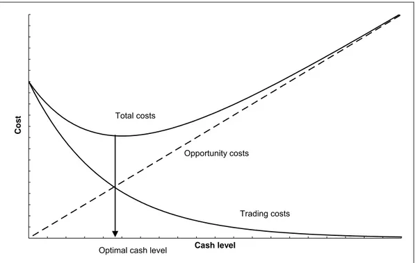
portfolio of marketable securities which can easily be converted into cash. In the Baumol model, the financial manager has to decide on the repartition of liquid funds between cash and marketable securities. Once again, there is a trade-off which constitutes the basis for the calculation. Yet, this trade-off is related to the opportunity costs of holding cash which increase along with the cash level and the trading costs which incur with every transaction and which decrease when the cash level increases.2
The opportunity costs represent the interests foregone for funds which are held in cash instead of being invested.3 The trading costs correspond to
fixed costs which incur when a company decides to either buy or sell marketable securities.4 If a company decides to maintain a low cash level
it will have to carry out many transactions leading to high trading costs but low opportunity costs because there are little idle cash funds.5 If it
maintains a high level of cash, the firm’s opportunity costs will be higher due to the relatively large amount of uninvested cash but the trading costs will decrease since only few transactions will be necessary.6 In line with
the EOQ model for inventory, the graph for determining the optimal level of cash will appear as follows:
1 cp. Brealey, R. & Myers, S. (2003), p. 891 2 cp. Ross, S. et al. (2008), p. 772
3 cp. ibid. at pp. 773-774 4 cp. ibid. at p. 774 5 cp. ibid. at p. 772 6 cp. ibid. at p. 774
Cash level
Cost
Opportunity costs
Trading costs Total costs
Optimal cash level
Figure 4: Graphic determination of the optimal cash level (draft)1
The optimal cash level has been determined graphically by identifying the minimum point of the total costs curve which again is defined by the addition of the opportunity costs and trading costs. This point can also be determined algebraically by differentiating the total costs equation which is defined as the addition of the two costs equations.2
2.3.2.2 Significance of the cash management model The Baumol model presents an approach for determining the optimal balance between cash and marketable securities. Therefore, it can be useful in order to illustrate the crucial elements of the issue of cash management. This issue consists in finding a balance between a firm’s cash holdings and the investment in marketable securities in order to optimize the availability of cash while maximizing the interest income for idle cash.
As it basically deals with the decision on the repartition of funds between investments of different liquidities, the model can be applied to the decision on the overall cash level, i.e. including cash equivalents. The associated costs would be similar, but a decision would have to be made between the investment in cash including cash equivalents and less liquid investments. Opportunity costs would be the same only that the foregone
1 adapted from: Ross, S. et al. (2008), p. 772 2 cp. Baumol, W. (1952), p. 548
returns would be related to any form of investment, with the exception of cash equivalents such as marketable securities. Trading costs would also be similar and would have to be generalized so as to contain all kinds of costs which occur when it is decided to liquidate an asset in order to generate cash.
2.3.3 Credit
management
Credit management deals with the firm’s decision on whether to grant credit to its customers and if so to determine the credit policy as well as the collection policy. 1 In this respect, decisions regarding credit management will have an impact on the selling firm’s level of accounts receivable. This is due to the fact that the terms of credit have an impact on its customers’ with less generous terms leading to decreased payment delays and thus augmented investment in accounts receivable and vice versa.2
2.3.3.1 Credit policy
Credit policies can vary significantly depending on the industry sector3, the
country of origin4 or the business’ seasonality.5 The terms of sale feature
the due date for net payment and an optional cash discount for payments within a certain period.6 For instance, terms of sale stated as ‘2/10, net 30’
imply that either a 2 percent cash discount can be taken advantage of by the buyer if payment occurs within 10 days from the invoice date or net payment should occur within 30 days.7 The longer the payment target and
the higher the cash discount, the more generous the terms of sale. The terms of sale therefore reflect the selling firm’s credit policy and its generosity. The selling firm’s motivation for granting cash discount in this respect is to accelerate collections in order to optimize cash availability.8
2.3.3.2 Optimal credit policy
Granting credit will have a positive impact on the firm’s turnover by stimulating sales but it will also generate costs of holding accounts receivable and create the risk of losses due to bad debts.9 The more generous the credit policy, the stronger the positive impacts on the firm’s
1 cp. Brealey, R. & Myers, S. (2003), p. 909 2 cp. Ross, S. et al. (2008), p. 797
3 cp. Brealey, R. & Myers, S. (2003), p. 909
4 cp. Intrum Justitia (2005), “European Payment Index – Spring 2005” 5 cp. Ross, S. et al. (2008), p. 795
6 cp. Brealey, R. & Myers, S. (2003), p. 910 7 cp. ibid.
8 cp. Ross, S. et al. (2008), p. 796 9 cp. ibid. at p. 802
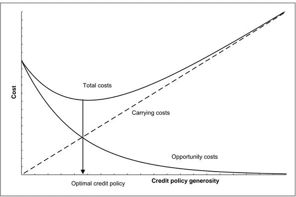
sales as well as on the associated costs.1 Therefore, the financial
manager’s task is to find the optimal credit policy which minimizes the total costs of credit. The total costs of credit are defined as the addition of opportunity costs which arise from lost sales and carrying costs of accounts receivable.2 Opportunity costs decrease when credit is extended
to customers as more and more customers are attracted to the company which generate increasing sales and therefore decrease opportunity costs of foregone sales.3 Carrying costs, however, increase in line with the
credit extension since these costs incur due to the cash collection delay, the relative cost of capital tie-up, the increased probability of bad debt losses and the costs of managing credit, all of which are positively related to credit extension.4 In this respect, the EOQ model is applicable to credit
management by relating credit policy to associated costs.5 Similarly to the
model for inventory, the illustration shows decreasing opportunity costs and increasing carrying costs for increasing level of credit policy generosity.6 The optimal credit policy can be found at the minimum point
of the total costs curve.7 The following graph illustrates this relationship in
a way similar to the models for inventory and cash:
Credit policy generosity
Cost
Carrying costs
Opportunity costs Total costs
Optimal credit policy
Figure 5: Graphic determination of the optimal credit policy (draft)8 1 cp. Ross, S. et al. (2008), p. 802 2 cp. ibid. 3 cp. ibid. 4 cp. ibid. 5 cp. ibid. 6 cp. ibid. 7 cp. ibid.
This graph demonstrates the basic relationship between credit policy generosity and associated costs which once again reflects the trade-off between risk and return which is common to all three types of current asset which are administered in working capital management. It should be noted that credit policy can influence several aspects of working capital management which are not contained in this simplified model and that the actual interrelation between the different variables is far more complex1
than this model suggests. Different more elaborate models which can incorporate many more aspects are at the disposal of the financial manager in order to decide on the firm’s optimal credit policy.2 However,
the purpose of the above illustration is merely to demonstrate the basic effect of credit policy on the associated carrying and opportunity costs and hereby establish a relationship between these costs.
2.3.3.3 Collection policy
Collection policy deals with the issue of collecting overdue receivables.3 This aspect copes with monitoring receivables and taking appropriate actions when the account is overdue.4 If a firm has an effective collection policy, this will reduce the probability of bad debts and decrease the cash collection period, hence decreasing the carrying costs of accounts receivable.5 This again will have an impact on the optimal credit policy. In other words, if the firm collects its accounts receivable efficiently, it can resort to a more profitable credit policy.6 The ‘average collection period’ or ‘days sales outstanding’ is a financial ratio which reflects the collection policy effectiveness by measuring “the average amount of time required to collect an account receivable”.7 By comparing the average collection period to the terms of sale the firm can keep track of its collection policy.8
2.3.4 Working
capital
policy
The overall way of managing working capital can differ significantly from firm to firm. Weston & Copeland refer to a company’s approach as “working capital policy”.9 Working capital policy involves the decision on
the level of current assets held by a company10 as well as the decision on
how these current assets ought to be financed.11 The latter will not be
1 cp. Weston, J. & Copeland, T. (1986), pp. 345-346 2 cp. ibid. at p. 346 3 cp. Ross, S. et al. (2008), p. 804 4 cp. ibid. at pp. 805-806 5 cp. Ross, S. et al. (2008), p. 806 6 cp. ibid. 7 ibid. at p. 804 8 cp. ibid. at p. 805
9 Weston, J. & Copeland, T. (1986), pp. 277-285 10 cp. ibid. at pp. 278-280
treated in this section as it is not of importance to the topic. Merely the investment in current assets and the optimal policy concerning the level of current assets will therefore be discussed in this section.
2.3.4.1 Investment in current assets
As shown above, the three components of working capital management imply separate yet similar associated costs and benefits. Therefore, it is evident that the level of current assets has an impact on the firm’s profitability. For instance, a large inventory ties up capital but it prevents the company from detrimental production stoppages due to stock-out. A high level of current assets therefore means less risk to the company but also lower earnings due to capital tie-up.1 Weston & Copeland refer to this interrelation as the “Risk-Return Tradeoff for Current Asset Investments”.2 Tables 3 and 4 excerpt from Weston & Copeland’s “Managerial Finance” ought to exemplify how different approaches to working capital management can influence a firm’s profitability. It shows figures resulting from three different policies, namely ‘conservative’, ‘middle-ground’ and ‘aggressive’ in two settings which are characterized by different assumptions.3 In this respect, the ‘conservative’ policy implies a higher ratio of current assets to sales while the ‘aggressive’ policy is characterized by a lower ratio of current assets to sales. The ‘middle-ground’ policy lies in between these two extremes. In Setting A, it is assumed that the working capital policy does not affect the EBIT rate as opposed to the situation in Setting B. Also, the working capital policies’ impact on sales is stronger in Setting B than in Setting A.
Setting A Conservative Middle-Ground Aggressive
Sales 110,000,000 105,000,000 100,000,000 EBIT (rate: 15%) 16,500,000 15,750,000 15,000,000 Current assets 70,000,000 55,000,000 40,000,000 Fixed assets 50,000,000 50,000,000 50,000,000 Total assets 120,000,000 105,000,000 90,000,000 Return on assets 13.75% 15.00% 16.67%
Table 3: Different working capital policies and impacts on return on assets (setting A)4
In Setting A, the aggressive policy would lead to the most profitable result in terms of return on assets. This is due to the fact that the negative impact on sales is less significant than the positive impact on asset
1 cp. Weston, J. & Copeland, T. (1986), p. 278 2 ibid.
3 cp. Weston, J. & Copeland, T. (1986), p. 279
structure, i.e. reducing current assets. However, as Setting B shows, this does not mean that the most aggressive policy is always optimal.
Setting B Conservative Middle-Ground Aggressive
Sales 115,000,000 105,000,000 80,000,000
EBIT rate 0.15 0.15 0.12
EBIT 17,250,000 15,750,000 9,600,000
Total assets 120,000,000 105,000,000 90,000,000
Return on assets 14.38% 15.00% 10.67%
Table 4: Different working capital policies and impacts on return on assets (setting B)1 In this case, the aggressive policy considerably reduces sales and also has a negative impact on the EBIT rate. The authors do not elaborate on the reasons for the fact that the EBIT rate is affected by the firm’s working capital policy. Presumably, the operating expenses increase significantly which could be due to uneconomic production stoppages caused by too little inventory, for instance. These increased costs again lower the EBIT. In Setting B, the decreased sales combined with the lower EBIT rate make the aggressive policy the least profitable one in terms of return on assets. This example shows that working capital management can have a considerable effect on profitability which is confirmed by quantitative studies.2 It also demonstrates that decision-makers should pay careful attention to the choice of policy since the negative effects of an aggressive policy can quickly outplay the positive ones.3
2.3.4.2 Optimal working capital policy
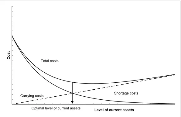
In order to determine the optimal policy, Ross et al. propose to integrate the different costs which are associated with the level of current assets in a model which then features carrying costs as well as shortage costs.4
Carrying costs are those costs which augment analogically with the level of current assets, e.g. opportunity costs.5 Shortage costs are those costs
which decrease when the level of current assets increases, i.e. costs which incur when current assets level is low, e.g. costs of running out of cash or inventory.6 If integrated in a diagram, these costs form curves
which are similar to those in the above discussed models.7 The optimal
1 excerpt from Weston, J. & Copeland, T. (1986), p. 279, Table 11.1
2 cp. Deloof, M. (2003), pp. 573-587; cp. Shin, H-H. & Soenen, L. (1998), “Efficiency of Working
Capital Management and Corporate Profitability”, Financial Practice and Education, Vol. 8, Issue 2, pp. 37-45
3 cp. Weston, J. & Copeland, T. (1986), p. 279 4 cp. Ross, S. et al. (2008), p. 752
5 cp. ibid.
6 cp. ibid. at p. 753
investment in current assets can be found at the minimum point of the total costs graph.1 Evidently, if “carrying costs are low or shortage costs are
high”2, the optimal level of current assets will be higher than in the
opposite case.3 The following illustrations demonstrate this relationship:
Level of current assets
Cost
Carrying costs
Shortage costs Total costs
Optimal level of current assets
Figure 6: Graphic determination of the optimal level of current assets (draft)4 The following figure displays the same relationship. However, the carrying costs are considerably lower than in figure 6:
1 cp. ibid. at p. 752 and p. 754 2 ibid. at p. 753
3 cp. ibid. at p. 753
Level of current assets
Cost
Carrying costs Shortage costs Total costs
Optimal level of current assets
Figure 7: Graphic determination of the optimal level of current assets with decreased carrying costs (draft)1
The decreased carrying costs lead to a higher optimal level of current assets as predicted by Ross et al. A similar increase of the optimal level of current assets would occur in case of an augmentation in shortage costs. This model can be consulted when the financial manager has to decide on the optimal investment in current assets.2 Yet, it does not contain all relevant aspects. There are many more elements and interrelations which influence the profitability of a working capital policy3, some of which are hardly measurable such as the impact of credit management on credit rating4, for instance. These aspects are definitely beyond the scope of this work. However, the basic relationships which have been described in this section ought to suffice for its aim which is to show the determinants and implications of a firm’s current assets level.
2.4 Cash
level
The following section aims at discussing cash level. For this purpose, the advantages and disadvantages are treated, potential determinants are discussed and a viewpoint on SMEs’ cash holdings is presented.
1 adapted from: Ross, S. et al. (2008), p. 754 2 cp. Ross, S. et al. (2008), p. 752
3 cp. Weston, J. & Copeland, T. (1986), p. 280 4 cp. Keown, A. et al. (2006), p. 478
2.4.1
Advantages & disadvantages of cash holding
The advantages of high cash level are numerous. The Keynesian motives which have been discussed in section 2.2 represent the basic reasons for holding cash.1 In this respect, these motives characterize the fundamental advantages of cash. A high level of cash allows the firm to easily carry out the regular expenses of its ordinary business activity and it also permits the company to pay for unforeseen expenses.2 If the cash level was too low and such an unexpected outflow occurred, the firm would have to either borrow the funds or forego the opportunity. Both alternatives obviously bring about significant costs. Short-term borrowing of funds can be extremely costly, e.g. trade credit financing3, and foregoing the opportunity results in opportunity costs which represent the lost return of the rejected investment. Another advantage of high cash level which shall be mentioned is the aspect of creditworthiness. The cash related financial ratios are a crucial element of credit rating and therefore a high level of cash will result in good creditworthiness.4 A strong credit standing will allow the firm to establish and maintain sound relationships with its suppliers and financial institutions, leading to advantageous benefits such as generous terms of purchase, for instance.5
The main disadvantage of a high cash level is the fact that it results in a significant capital tie-up. This is due to the fact that the funds that are used to maintain the cash holding at a high level can not be invested profitably.6 Hence, a disadvantage of a high cash level is the aspect of foregone longer-term investments which create opportunity costs.7 For instance, if a company pursues a policy of high cash level with a high safety stock of liquid funds, this can lead to unprofitable investment decisions if a potential longer-term investment is rejected in favour of the maintenance of cash.8
2.4.2
The determinants of cash level
Several studies have been conducted in order to detect determinants of cash level, i.e. factors which influence the amount of cash that is held by a firm. The issue has been a matter of interest for a long time with Frazer’s
1 cp. Keynes, J. (1973), pp. 195-196 2 cp. Ross, S. et al. (2008), p. 771 3 cp. Van Horne, J. (1995), pp. 448-449 4 cp. Weston, J. & Copeland, T. (1986), p. 292 5 cp. ibid.
6 cp. Keynes, J. (1973), p. 196 7 cp. Ross, S. et al. (2008), p. 752 8 cp. Keynes, J. (1973), p. 196
study1 dating back to the year 1964. The aim of the following section is to
present the theoretical view on the determinants of cash level by discussing relevant studies which have been conducted in this field.
The articles which have been analyzed investigated corporate cash holdings by means of quantitative studies which share a similar methodology, namely the analysis of financial information of a large sample of firms. Obviously, in the examined articles, cash level has been measured by a ratio – relative to total assets2, for instance – and not as an
absolute figure. Based on the methodology and the scientific background, the results can be evaluated as reliable. This is further confirmed by the fact that there are considerable congruencies among the different researchers’ findings.
In order to simplify matters, the following tables recapitulate the main findings of these relevant scientific articles. The purpose of the tables is to give a brief overview of previous research in the field of cash level determinants in a compiled form. Presenting the numerous theoretical foundations in detail or discussing each single study’s findings would clearly go beyond the scope of this work. The tables merely take factors into consideration which have been confirmed by more than one empirical study. This approach should allow the identification of the most important factors since many more could be imagined and have been analyzed by the mentioned authors.
First, factors which are positively related to cash level, i.e. factors which increase the cash level when their intensity is enhanced, are being presented.
1 cp. Frazer, W. (1964), “The Financial Structure of Manufacturing Corporations and the Demand
for Money: Some Empirical Findings”, The Journal of Political Economy, Vol. 72, Issue 2, pp. 176-183
2 cp. Opler, T.; Pinkowitz, L.; Stulz, R.; Williamson, R. (1999), “The determinants and implications of