http://www.diva-portal.org
Postprint
This is the accepted version of a paper presented at 14th International Congress, Geological Society of
Greece, Thessaloniki, May 2016.
Citation for the original published paper:
Adamaki, A., Roberts, R. (2016)
EVIDENCE OF PRECURSORY PATTERNS IN AGGREGATED TIME SERIES.
In: Bulletin of the Geological Society of Greece, vol. L, 2016, Proceedings of the 14th Intern.
Congress, Thessaloniki, May 2016
N.B. When citing this work, cite the original published paper.
Permanent link to this version:
Δελτίο της Ελληνικής Γεωλογικής Εταιρίας, τόμος L, 2016
Πρακτικά 14ου Διεθνούς Συνεδρίου, Θεσσαλονίκη, Μάιος 2016 Bulletin of the Geological Society of Greece, vol. L, 2016 Proceedings of the 14th Intern. Congress, Thessaloniki, May 2016
EVIDENCE OF PRECURSORY PATTERNS IN
AGGREGATED TIME SERIES
Adamaki K.A.
1and Roberts R.G.
11Uppsala University, Department of Earth Sciences, SE-752, Uppsala, Sweden, angeliki.adamaki@geo.uu.se, roland.roberts@geo.uu.se
Abstract
We investigate temporal changes in seismic activity observed in the West Corinth Gulf and North-West Peloponnese during 2008 to 2010. Two major earthquake sequences took place in the area at that time (in 2008 and 2010). Our aim is to analyse Greek seismicity to attempt to confirm the existence or non-existence of seismic precursors prior to the strongest earthquakes. Perhaps because the area is geologically and tectonically complex, we found that it was not possible to fit the data well using a consistent Epidemic Type Aftershock Sequence (ETAS) model. Nor could we unambiguously identify foreshocks to individual mainshocks. Therefore we sought patterns in aggregated foreshock catalogues. We set a magnitude threshold (M3.5) above which all the earthquakes detected in the study area are considered as “mainshocks”, and we combined all data preceding these into a single foreshock catalogue. This reveals an increase in seismicity rate not robustly observable for individual cases. The observed effect is significantly greater than that consistent with stochastic models, including ETAS, thus indicating genuine foreshock activity with potential useful precursory power, if sufficient data is available, i.e. if the magnitude of completeness is sufficiently low.
Keywords: Corinth Gulf, Seismicity, Aggregated Foreshock Catalogues.
Περίληψη Μελετάμε χρονικές μεταβολές της σεισμικής δραστηριότητας στο Δυτικό Κορινθιακό Κόλπο και τη Βορειοδυτική Πελοπόννησο κατά τα έτη 2008-2010. Δύο σημαντικές σεισμικές ακολουθίες σημειώθηκαν στην περιοχή σε αυτή την περίοδο (2008 και 2010). Στόχος είναι να αναλύσουμε τη σεισμικότητα ώστε να επιβεβαιώσουμε την ύπαρξη ή μη προσεισμικής δραστηριότητας πριν από τους μεγαλύτερους σεισμούς. Λόγω της γεωλογικής και τεκτονικής πολυπλοκότητας της περιοχής, δεν ήταν εφικτή η εφαρμογή ενός ενιαίου μοντέλου Επιδημικού Τύπου Μετασεισμικών Ακολουθιών (ETAS), ούτε η αναγνώριση προσεισμών μεμονωμένων κυρίων σεισμών. Επομένως, αναζητήσαμε ανάλογα μοτίβα σε ενιαίους καταλόγους προσεισμών. Θέσαμε ένα μέγεθος (Μ3.5) πάνω από το οποίο όλοι οι σεισμοί θεωρούνται “κύριοι”, και συνδυάσαμε τα δεδομένα που προηγούνται αυτών, σε ένα κοινό κατάλογο. Αναδεικνύεται έτσι μια αύξηση του ρυθμού σεισμικότητας που δεν είναι εμφανής σε μεμονωμένες περιπτώσεις και είναι πιο σημαντική από εκείνη που προβλέπεται από στοχαστικά μοντέλα, όπως το ETAS, υποδηλώνοντας την ύπαρξη προσεισμών που μπορούν να δώσουν τη δυνατότητα πρόγνωσης αν υπάρχει ικανοποιητικό πλήθος δεδομένων, δηλ. αν το μέγεθος πληρότητας είναι αρκετά χαμηλό. Λέξεις κλειδιά: Κορινθιακός Κόλπος, Σεισμικότητα, Ενιαίοι Κατάλογοι Προσεισμών.
1. Introduction - Background
A major question in seismology is if it is possible to develop reliable short-term forecasting of strong earthquakes, and if so, how. Many phenomena prior to large events have been investigated in order to assess their possible predictive value, but generally with limited success. A group of such phenomena are those related to temporal changes in seismicity patterns preceding large events. In order to identify temporal changes as potential precursory phenomena, it is necessary to know the seismicity pattern that is expected if no large event is imminent. Numerous studies have investigated “background” (or “reference”) seismicity, mostly assuming stationarity of the process (e.g. Toda et
al., 1998; Toda and Stein, 2003). However, any temporal clustering e.g. due to aftershock sequences
with decaying seismicity rates according to the empirical Omori law, will lead naturally to non-stationary time series (Marsan and Nalbant, 2005). Declustering techniques (e.g. the Reasenberg (1985) algorithm or the stochastic declustering of Zhuang et al., 2002) aim to identify and remove the aftershocks from seismicity catalogues, but their success may depend on the validity of the assumptions made in the analyses.
Seeking patterns of foreshock activity preceding large events is an important topic for prediction research. Earthquakes demonstrate ongoing deformation. An area that is subjected to shear loading may either deform gradually, seismically or aseismically, or lock. The latter implies the accumulation of stress which may later lead to a large event. This implies that relative seismic quiescence may have some predictive information regarding large events. Unfortunately, it is generally difficult to distinguish true quiescence from other phenomena, for example decaying aftershock sequences. Foreshocks to large events, i.e. small events above background level preceding larger events, are often reported - but usually only retrospectively. The fundamental predictive value of foreshocks is sometimes questioned (see Mignan, 2014 for a review). For example, in cascade models (Felzer et al., 2015; Helmstetter et al., 2003), such as the Epidemic Type Aftershock Sequence (ETAS) model, mainshocks are considered to be aftershocks of smaller mainshocks (i.e. the foreshocks), and all events have a magnitude “chosen” at random from a given distribution. If such models are correct, foreshocks contain little or no precursory information. Many Greek earthquake sequences have been analysed using various statistical methods, investigating seismicity rate changes on short or long time scales, and by applying temporal or spatio-temporal modeling (e.g. Adamaki et al., 2010, 2011; Console et al., 2006; Papadimitriou et
al., 2012). Latoussakis and Drakatos (Drakatos and Latoussakis, 1996; Latoussakis and Drakatos,
1994) found evidence of seismic quiescence before strong earthquakes that occurred within several aftershock sequences in Greece. Papadopoulos et al. (2000) identified foreshock activity during less than 4 months prior to 12 out of 17 strong earthquakes (M>5) around the Corinth Gulf. Gospodinov
et al. (2015) recently presented a day by day forecast of seismicity working with data in the
Kefalonia area. Here, we use interevent times between earthquakes within a specified area as a time-specific proxy for seismicity rate.
To identify stationary background or “reference” seismicity for the given area we may seek time periods with no apparent rate changes. However, even if there are such periods, containing e.g. no significant aftershock sequences, spurious temporal changes may be observed due to changes in both observing networks and the methods used to detect, locate and analyse events. One way to minimize these effects is to use fairly short and recent time periods.
The most common model of seismicity is a homogeneous Poisson process combined with triggered aftershock activity described by the well known Omori law. The modified formula introduced by Utsu (1969).
Equation 1 - Modified Omori Formula (MOF)
gives the aftershock rate n(t) as a function of time. K, c and p are empirical constants. Later, Ogata (1988) introduced the ETAS model where all aftershocks can produce their own aftershocks, where the seismicity is described by
Equation 2 - Formula for ETAS
λ(t)=μ+K*exp(a(Mi-Mmin))/(c+t-ti)p
μ represents the background seismicity, tj are the occurrence times of the events with magnitudes mj that took place before time t, m0 is the cut-off magnitude of the data (usually equal to the completeness magnitude mc) above which all events can produce secondary aftershocks, and α is a measure of the efficiency of a shock in generating aftershock activity relative to its magnitude. The parameters are estimated using the maximum likelihood method and the goodness of fit is usually tested with residual analysis (Ogata, 1999). Several versions of ETAS modeling have been developed aiming at better explaining observed seismicity. Gospodinov and Rotondi (2006) for example suggested the Restricted ETAS model (RETAS), where only earthquakes above a cut-off magnitude (which can be higher than mc) can produce their own aftershocks. Implicit in all these models is that all events can be considered as foreshocks, mainshocks and aftershocks (Helmstetter
et al., 2003).
Seismicity data is complex and statistical tools must be used to compare observations (related to potential precursors) to what is predicted by cluster-type models like the ETAS (Bouchon et al., 2013; Marsan et al., 2014; Ogata and Katsura, 2014). Below, we apply both established and new methods to Greek data to investigate the occurrence of foreshocks.
2. Data
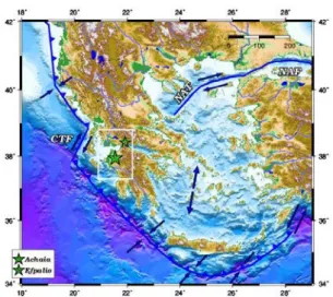
We use events from 2008 to 2010 in the western part of the Corinth Gulf and the northwestern part of the Peloponnese (white rectangle in Figure 1) listed in the catalogue published by the Aristotle University of Thessaloniki, which includes only earthquakes with magnitudes bigger than 2.0, recorded by the Hellenic Unified Seismological Network. Our data set includes 4690 events, including 3 major events, a) the strong earthquake in Achaia (NW Peloponnese) in 2008 (M>6.0) and b) the doublet of M>5.0 events that occurred at Efpalio (W Corinth Gulf) in 2010. The epicenters of these are shown in Figure 1 (see Karakostas, 2009; Karakostas et al., 2012 and Sokos et al., 2012 for more details on these sequences).
The application of the ETAS model requires a complete catalogue. Therefore, using the methods of Leptokaropoulos et al. (2013), the completeness magnitude was estimated for different parts of the dataset, with the highest value equal to 2.6. That the 2010 earthquakes occurred within the positive lobe of the Coulomb stress changes that followed the 2008 strong event (Karakostas, 2009) and the observed seismicity migrated towards the area of Efpalio between 2008 and 2010 suggests that the events are related. Segou et al. (2014) performed static stress transfer calculations and concluded that it's likely that the Achaia event in 2008 promoted the Efpalio sequence in 2010.
3. Temporal evolution of Seismicity
In Figure 2 we show rate histograms of our data, i.e. the number of events in fixed time bins. The red lines represent an Omori type rate to be compared to the observed decay of seismicity after the large events. The first 2 months of the 2008 aftershock sequence are characterized by a strongly decaying rate, as seen in Figure 2b, which is followed by generally lower seismicity rate (compare to the previous part) until the beginning of 2010. Almost 40% of the events during this interval occurred around Efpalio. In Figure 2c we can see that the decay rate of the second aftershock
Figure 1 – The study area (white rectangle). The two stars show the epicentres of the major events during 2008-2010 (Achaia, 2008 and Efpalio, 2010). Blue arrows and lines, tectonic
motions and features: NAF: North Anatolian Fault, NAT: North Aegean Trough, CTF: Cephalonia Transform Fault. Arrows: approximate direction of relative plate motion.
sequence is rather rapid, as the number of earthquakes in each bin reaches relatively low values only 1.5 months after the M>5 events. We see that an Omori type decay of power 1 can only approximately describe the observed processes.
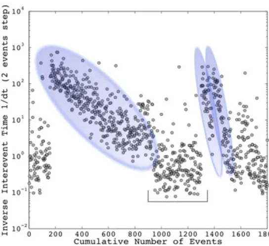
Such rate plots are useful, but the large changes in rate mean that while some bins contain very few points others contain many, and possibly relevant details of time evolution within these bins cannot be seen. Therefore we estimate the rate as the inverse of the average interevent time for one or a few temporally neighboring events, allowing many rate samples where rate is high. Figure 3 shows the inverse interevent times versus the sequential event number for our whole data set, yielding a clearer image of the rate decay that follows the occurrence of each larger event. The first area marked in Figure 3 corresponding to a period of almost 2 months following the Achaia main-shock shows that the seismicity decays rather steadily while at later times (the interval marked between the shaded areas) there aren't any obvious rate changes until the doublet events occur. In the next shaded area we can see the initial decay that follows the first doublet earthquake and after the second of the doublet events the rate essentially monotonically decays for about 1.5 months. In the last part of the dataset the activity seems to be dominated by 4 M>4 events and their aftershocks (Figure 3).
4. ETAS analysis
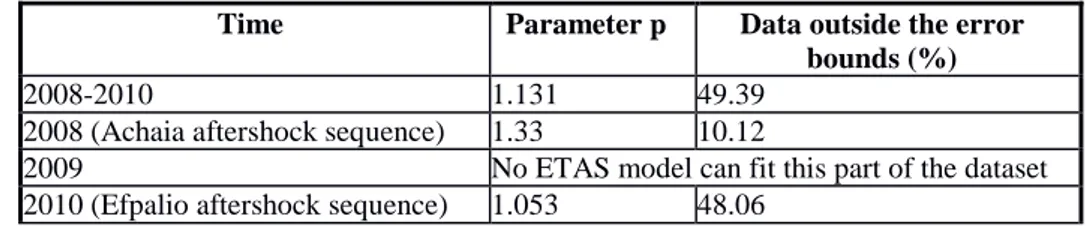
These simple presentations of our data provide some evidence that the process is not homogeneous. Several intervals seem to be related to different rates and as a result they introduce rate changes that can be further tested. With the help of the algorithm Gospodinov and Rotondi (2006), developed, we applied the ETAS model to the whole dataset and to subsets. For the complete 2008-2010 time period, although the Akaike criterion (Akaike, 1974) indicated that the the ETAS model fitted well compared to MOF and RETAS, much of the data were outside the error bounds of the estimation the model provided, implying that a single ETAS model is inadequate to describe the data. Therefore we modelled separately three different time intervals, a) following the 2008 major event in Achaia, b) during 2009 when no strong earthquakes occurred and c) following the doublet in Efpalio. The fit was poor in the last two cases, although we tried applications assuming several magnitude thresholds. A summary of the results can be seen in Table I. Although there are parts of the dataset where the right choice of parameters (equation 2) can model the real seismicity well, the results are not stable in most of the cases. Specifically, when a long period is chosen the model underestimates the intense aftershock activity while overestimating rate where the rate doesn't change significantly.
The best fit was achieved for the months following the 2008 major event (M>6), although the decay was underestimated during the first days of the aftershock sequence. The values of parameter p shown in Table 1 indicate that the decay rate decreases over time. Michas et al. (2014) also found that the period following the Efpalio doublet was characterized by some kind of homogeneity compare to the period before that. These observations could imply that there are different processes occurring during the time we study, even before the major events of 2010 when no major earthquakes occurred.
Figure 2 - a) Histogram of the seismicity observed in the study area during 2008-2010, b) A more detailed picture of the 2008 aftershock sequence, c) Same as in b) but for the 2010
aftershock sequence. The red lines show the Omori type decay with p=1.
Table 1 - Summary of results after applying the ETAS model on the dataset and on subsets.
Time Parameter p Data outside the error bounds (%)
2008-2010 1.131 49.39
2008 (Achaia aftershock sequence) 1.33 10.12
2009 No ETAS model can fit this part of the dataset
Figure 3 - The inverse interevent time against the sequential earthquake number. The shaded areas show the aftershocks that followed each of the major events (i.e. the mainshock
in Achaia and the doublet in Efpalio), while the marked area between them corresponds to the seismicity observed during 2009 (where no major events occurred).
5. Aggregated Time Series
Analyses based on ETAS or examination of data such as Figures 2 and 3 was not able to reveal any unambiguous anomalous activity prior to the larger events. An important question is if this is because no such activity is present, or because our data is insufficient to reveal such effects, Therefore, we chose to superimpose data preceding and following all larger events in our catalogue, hoping that the averaging involved will reveal patterns otherwise obscured due to e.g. the difficulty in assessing if a burst of activity prior to a given mainshock is “precursory” or some unrelated phenomenon. Clearly, when averaging over events, unrelated phenomena should tend to be temporally evenly distributed. A magnitude threshold was chosen, and all events of this magnitude or higher considered to be “mainshocks”. Such events which, within a specified time window, were preceded by a larger event were excluded. Events before and after the remaining “mainshocks” and spatially close to these were placed into a common catalogue, with time relative to each mainshock. We can then examine the aggregated rate to see if there is a general increase or period of quiescence prior to our “mainshocks”. Note that we make no attempt to separate aftershocks and other events, and larger events in aftershock sequences may be included as “mainshocks”, as long as they are not close in time to a larger preceding event.
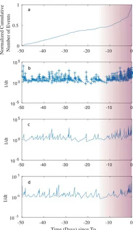
We choose to focus on the intervals after the 2008 M6.4 event and the doublet in 2010. In the example shown in Figure 4, all other earthquakes with magnitudes above Mth=3.5 are regarded as main shocks, and events for the preceding 50 days and within 10 km radius were aggregated. This approach should be robust to technical changes in networks and analysis, as these will generally be stable for each 50 day data subset. As mentioned above, even if Mc changes over time we can reasonably assume that there aren't significant changes in Mc within the short intervals preceding these "mainshocks". In Figure 4, the top plot (a) shows the normalized cumulative number of events of the aggregated series, plotted against the time preceding the mainshock times T0. The shaded area of the last 15 days prior to T0 is of interest as here the seismicity rate apparently increases. In Figure 4b we also present the inverse interevent times for the events in the aggregated time series, plotted against time. We can see a clear increase in seismicity rate about 2 weeks before T0.
Figure 4 - Aggregated preshock sequences for “mainshocks” of M>3.5. a) The normalized cumulative number of events against time, b) The inverse interevent times of the common series, c) and d) The aggregated series is divided in two random parts. The shaded areas show the increase in seismicity during the last days before T0, which is observed in all plots.
Especially as the rate before and after different larger events may be very different, we must assess if any apparent general patterns of behavior are artefacts e.g. due to one or a few events dominating the aggregated series. We performed various tests to evaluate this, including randomly splitting the main shocks into two separate groups and comparing results, and performing calculations including events of different magnitude. Such tests included choice of the threshold for the identification of “mainshocks” and use of data only from selected magnitude bands in the histograms. Examples are shown in Figure 4 (c and d). An increased seismicity rate was consistently seen.
If seismicity consists of events completely random in time, each of which may have aftershocks, then we expect no increase in activity prior to larger events. In such a case, we can test if an observed increase in seismicity prior to larger events is significant by performing numerical random simulations, and seeing how often these produce a similar increase by chance. For ETAS models, it is more complex. The ETAS model implies that a higher activity rate indicates a higher future rate, which in turn implies increased risk of a large event, as the magnitude of each new event is randomly “chosen” from a Gutenberg-Richter distribution. This randomness means that rate increases prior to larger events should be observed, but that these are essentially not useful for predicting large coming events. Therefore, if a rate increase prior to larger events is observed, it is important to assess if this is what we would expect from an ETAS model. We can also test this using numerical random simulations.
Here, in order to assess if the observed acceleration is what we would expect from ETAS-type behaviour, we also run a randomized test on our empirical data. In the ETAS model, the probability of a new event is steered by earlier events, but the magnitude of the new event is not. Therefore ETAS-consistent rate increases should be observed even if we select our “mainshocks” completely at random from our catalogue, independently of their magnitude. For simple comparison, we test with the same number of randomly selected events as in our actual mainshock analysis, but repeat this many times which allows us to define empirical confidence limits. This simple but robust test of the ETAS rate increase hypothesis showed that although there is a rate increase in the aggregated data which is consistent with the ETAS model, this is only visible for the last two days of the stacked preshock sequence. Thus, the clear rate increase seen in Figure 4 can not be explained in this manner. Our empirical confidence tests indicate that this can be stated at a very high confidence level of well over 95%.
6. Discussion - Conclusion
Our analysis was motivated by the two earthquake sequences (Achaia and Efpalio) that occurred close in time (2008 and 2010) and space (NW Peloponnese and W Corinth Gulf), where both Coulomb stress transfer calculations and the observed apparent migration of seismicity from Achaia to Efpalio indicate that the two sequences may be causally related. These sequences are fairly recent, implying relatively high sensitivity and data quality from the Greek network, and a rather homogeneous catalogue with a relatively low completeness magnitude.
Investigating the sequences in more detail, we found that in the aftershock sequence of the 2008 event in Achaia the rate decays fast in the short term after the main-shock (almost 2 months) and is followed by a lower seismicity period. After this time, this (power-law) decay of rate apparently changes. For the 2010 sequence the p value is lower than for the 2008 event, and is very close to 1. No ETAS model could reproduce well the seismicity for the whole data set. Subsets of data were selected according to where apparently significant changes in behaviour were observed and the ETAS model was applied separately to each of these. For these subsets, ETAS was able to fit the data successfully in some cases. For even shorter time periods there were too few events to apply ETAS.
Thus, while the data appears to be piece-wise consistent with the concept of poissonian background seismicity and aftershock sequences consistent with Omori- and ETAS-type behavior, there are additional and apparently significant components in the tempo-spatial evolution of seismicity. The data may contain foreshocks to the largest events investigated, but with so few data no preshock sequences to these could be unambiguously identified. Therefore, rather than trying to identify foreshocks to these events specifically, we aggregated data to assess if generic foreshock activity exists, and if so what its character is. Treating many slightly larger events (M>3.5) as mainshocks, and superimposing activity prior to these, produces an aggregated time series. These analyses show an increase in seismicity rate prior to main shock time. The rate increase appears to be consistent with the statistical inverse Omori law (Helmstetter and Sornette, 2003) only to a limited extent. This implies that foreshock activity is common, perhaps even ubiquitous, even though it is often not possible for individual main shocks to distinguish foreshocks from other seismicity such as a smaller event with some aftershocks prior to a main shock. These observations suggest that there are structural components in the seismicity which are not consistent with the normal ETAS model concept, as well as supporting the idea that foreshocks may very well ultimately provide a tool for more routine short-term prediction of coming larger events. In other words, there is in some sense an increase in seismicity prior to major events, and this has a character suggesting that it might be a useable basis for producing short-term prognoses of coming larger events. It does not, however, follow automatically from our results that such prognosis is possible. What does seem clear is that for any real chance of observing and identifying precursors to coming events very high quality data (including very low Mc) will be necessary.
7. Acknowledgments
We would like to thank Prof. Ólafur Gudmundsson and Silvia Salas Romero from the Geophysics Department of Uppsala University, whose comments helped improving the initial manuscript.
8. References
Adamaki, A.K., Tsaklidis, G.M., Papadimitriou, E.E. and Karakostas, V.G., 2010. Evidence for induced seismicity following the 2001 Skyros mainshock, Bull. Geol. Soc. Greece, 43, 1983-1993.
Adamaki, A., Papadimitriou, E., Tsaklidis, G. and Karakostas, V., 2011. Statistical properties of aftershock rate decay: Implications for the assessment of continuing activity, Acta Geophys., 59, 748-769.
Akaike, H., 1974. A new look at the statistical model identification, IEEE Trans. Autom. Control, 19, 716-723. doi: 10.1109/TAC.1974.1100705.
Bouchon, M., Durand, V., Marsan, D., Karabulut, H. and Schmittbuhl, J., 2013. The long precursory phase of most large interplate earthquakes, Nat. Geosci., 6, 299-302, doi: 10.1038/ngeo1770. Console, R., Rhoades, D.A., Murru, M., Evison, F.F., Papadimitriou, E.E. and Karakostas, V.G., 2006. Comparative performance of time-invariant, long-range and short-range forecasting models on the earthquake catalogue of Greece, J. Geophys. Res. Solid Earth, 111, B09304, doi: 10.1029/2005JB004113.
Drakatos, G. and Latoussakis, J., 1996. Some features of aftershock patterns in Greece, Geophys. J.
Int., 126, 123-134. doi: 10.1111/j.1365-246X.1996.tb05272.x.
Felzer, K.R., Page, M.T. and Michael, A.J., 2015. Artificial seismic acceleration, Nat. Geosci., 8, 82-83, doi: 10.1038/ngeo2358.
Gospodinov, D., Karakostas, V. and Papadimitriou, E., 2015. Seismicity rate modeling for prospective stochastic forecasting: the case of 2014 Kefalonia, Greece, seismic excitation,
Nat. Hazards, 1-20. doi: 10.1007/s11069-015-1890-8.
Gospodinov, D. and Rotondi, R., 2006. Statistical Analysis of Triggered Seismicity in the Kresna Region of SW Bulgaria (1904) and the Umbria-Marche Region of Central Italy (1997), Pure
Appl. Geophys., 163, 1597-1615, doi: 10.1007/s00024-006-0084-4.
Helmstetter, A., Ouillon, G. and Sornette, D., 2003. Are aftershocks of large Californian earthquakes diffusing? J. Geophys. Res. Solid Earth, 108, 2483, doi: 10.1029/2003JB002503.
Helmstetter, A. and Sornette, D., 2003. Importance of direct and indirect triggered seismicity in the ETAS model of seismicity, Geophys. Res. Lett., 30, 1576, doi: 10.1029/2003GL017670. Karakostas, V., 2009. Seismicity patterns before strong earthquakes in Greece, Acta Geophys., 57,
367-386.
Karakostas, V., Karagianni, E. and Paradisopoulou, P., 2012. Space-time analysis, faulting and triggering of the 2010 earthquake doublet in western Corinth Gulf, Nat. Hazards, 63, 1181-1202, doi: 10.1007/s11069-012-0219-0.
Latoussakis, J. and Drakatos, G., 1994. A quantitative study of some aftershock sequences in Greece,
Pure Appl. Geophys., 143, 603-616, doi: 10.1007/BF00879500.
Leptokaropoulos, K.M., Karakostas, V.G., Papadimitriou, E.E., Adamaki, A.K., Tan, O. and İnan, S., 2013. A Homogeneous Earthquake Catalog for Western Turkey and Magnitude of Completeness Determination, Bull. Seismol. Soc. Am., 103, 2739-2751, doi: 10.1785/0120120174.
Marsan, D., Helmstetter, A., Bouchon, M. and Dublanchet, P., 2014. Foreshock activity related to enhanced aftershock production, Geophys. Res. Lett., 41, 2014GL061219, doi: 10.1002/2014GL061219.
Marsan, D. and Nalbant, S.S., 2005. Methods for Measuring Seismicity Rate Changes: A Review and a Study of How the M w 7.3 Landers Earthquake Affected the Aftershock Sequence of the M w 6.1 Joshua Tree Earthquake, Pure Appl. Geophys., 162, 1151-1185, doi: 10.1007/s00024-004-2665-4.
Michas, G., Sammonds, P. and Vallianatos, F., 2014. Dynamic Multifractality in Earthquake Time Series: Insights from the Corinth Rift, Greece, Pure Appl. Geophys., 172, 1909-1921, doi: 10.1007/s00024-014-0875-y.
Mignan, A., 2014. The debate on the prognostic value of earthquake foreshocks: A meta-analysis,
Sci. Rep., 4, doi: 10.1038/srep04099.
Ogata, Y., 1999. Seismicity Analysis through Point-process Modeling: A Review, Pure Appl.
Geophys., 155, 471-507, doi: 10.1007/s000240050275.
Ogata, Y., 1988. Statistical Models for Earthquake Occurrences and Residual Analysis for Point Processes, J. Am. Stat. Assoc., 83, 9-27, doi: 10.1080/01621459.1988.10478560.
Ogata, Y. and Katsura, K., 2014. Comparing foreshock characteristics and foreshock forecasting in observed and simulated earthquake catalogs, J. Geophys. Res. Solid Earth, 119, 2014JB011250, doi: 10.1002/2014JB011250.
Papadimitriou, E., Gospodinov, D., Karakostas, V. and Astiopoulos, A., 2012. Evolution of the vigorous 2006 swarm in Zakynthos (Greece) and probabilities for strong aftershocks occurrence, J. Seismol., 17, 735-752, doi: 10.1007/s10950-012-9350-3.
Papadopoulos, G.A., Drakatos, G. and Plessa, A., 2000. Foreshock activity as a precursor of strong earthquakes in Corinthos Gulf, Central Greece, Phys. Chem. Earth Part Solid Earth Geod., 25, 239-245, doi: 10.1016/S1464-1895(00)00039-9.
Reasenberg, P., 1985. Second-order moment of central California seismicity, 1969-1982, J.
Geophys. Res. Solid Earth, 90, 5479-5495, doi: 10.1029/JB090iB07p05479.
Segou, M., Ellsworth, W.L. and Parsons, T., 2014. Stress Transfer by the 2008 Mw 6.4 Achaia Earthquake to the Western Corinth Gulf and Its Relation with the 2010 Efpalio Sequence, Central Greece, Bull. Seismol. Soc. Am., 104, 1723-1734, doi: 10.1785/0120130142.
Sokos, E., Zahradník, J., Kiratzi, A., Janský, J., Gallovič, F., Novotny, O., Kostelecký, J., Serpetsidaki, A. and Tselentis, G.-A., 2012. The January 2010 Efpalio earthquake sequence in the western Corinth Gulf (Greece), Tectonophysics, 530-531, 299-309, doi: 10.1016/j.tecto.2012.01.005.
Toda, S. and Stein, R., 2003. Toggling of seismicity by the 1997 Kagoshima earthquake couplet: A demonstration of time-dependent stress transfer, J. Geophys. Res. Solid Earth, 108, 2567, doi: 10.1029/2003JB002527.
Toda, S., Stein, R.S., Reasenberg, P.A., Dieterich, J.H. and Yoshida, A., 1998. Stress transferred by the 1995 Mw = 6.9 Kobe, Japan, shock: Effect on aftershocks and future earthquake probabilities, J. Geophys. Res. Solid Earth, 103, 24543-24565, doi: 10.1029/98JB00765. Utsu, T., 1969. Aftershocks and Earthquake Statistics (1): Some Parameters Which Characterize an
Aftershock Sequence and Their Interrelations, J. Fac. Sci. Hokkaido Univ. Ser. 7 Geophys., 3, 129-195.
Zhuang, J., Ogata, Y. and Vere-Jones, D., 2002. Stochastic Declustering of Space-Time Earthquake Occurrences, J. Am. Stat. Assoc., 97, 369-380, doi: 10.1198/016214502760046925.