3D FINITE ELEMENT MODELING OF LABORATORY HYDRAULIC FRACTURE EXPERIMENTS
by
ii
A thesis submitted to the Faculty and the Board of Trustees of the Colorado
School of Mines in partial fulfillment of the requirements for the degree of Master of
Science (Petroleum Engineering).
Golden, Colorado Date: __________ Signed:
________________
Naif Alqahtani Signed:________________
Dr. Jennifer L. Miskimins Thesis Advisor Golden, Colorado Date:________
Signed:________________
Dr. Ramona M. Graves Professor and Head Department of Petroleum Engineeringiii
ABSTRACT
This study is the fourth phase of a fracture growth and height containment
project conducted as part of the FAST Consortium in the Petroleum Engineering
Department at the Colorado School of Mines. In this phase, finite element modeling
(FEM) of stress analyses design, results and observations of seven different
homogeneous and laminated block models are presented. The purpose of this work
is to study the effects of stress loading on fracture growth in the laboratory scale
conditions, and determine how to best apply these results in in-situ formations. The
primary objectives of this study are using the finite element modeling to evaluate the
effects of varying load paths on stresses setup or created due to triaxial loading and
compare them with previously conducted laboratory results. In addition, the impact
of extrapolating the effects on extrapolating laboratory results to field in-situ settings
is determined.
The seven basic block systems created include a one layer with and without
a wellbore, as a control case; a three model layer with and without a wellbore; and
three model blocks with seven layers with and without a wellbore in addition to a
wellbore with steel casing. Finite element modeling of the stressed laminated block
illustrated that stress contrasts are set up spatially (inside individual layers as well as
across layers) due to the material property contrasts and the vertically and triaxially
stressed state of the blocks. Development of shear stresses was also seen at the
iv
Lab work and observations conducted by Athavale in 2007 were interpreted
numerically by looking at the stress distribution across the seven layer blocks
representing the block used experimentally. These models show stress variations
indicating a possibility of fractures to would initiate and propagate perpendicular to the minimum horizontal stress (σ3) in the east-west direction of the investigated block. The shear stresses around the wellbore affect the fractures growth, it was
indicated experimentally that fracture grows away from the wellbore but with
somewhat deviated direction from the maximum horizontal stress as it grows to the
edges, the model shows shear stress variation that explain the fracture path
deviation. This agrees well with the experimental observation with the upper tip of
the fracture contained in the cement layer (second from top) which is has the higher σ3 value as indicated by the model and the experiment.
v
TABLE OF CONTENTS
ABSTRACT ... iii
LIST OF FIGURES ... viii
LIST OF TABLES ...xv
ACKNOWLEDGMENTS ... xvi
CHAPTER 1: INTRODUCTION ...1
1.1 Research Objectives ...2
1.2 Previous Project Work ...2
1.3 Motivation and Context ...3
CHAPTER 2: LITERATURE REVIEW ...5
2.1 Hydraulic Fracturing ...5
2.2 Hydraulic Fracture Propagation ...6
2.3 Stress Effects ...11
2.4 Effects of Reservoir Depletion ...13
2.5 Brief Summary of Previous Project Works ...14
CHAPTER 3: FINITE ELEMENT METHOD ...19
3.1 A Brief History of the Method ...19
3.2 The Finite Element Method ...19
vi
3.4 A General Procedure for Finite Element Analysis ...25
3.4.1 Preprocessing ...25
3.4.2 Solution ...26
3.4.3 Postprocessing...26
3.5 The Future of this Method ...27
CHAPTER 4: FINITE ELEMENT MODELING...28
4.1 Modeling Software...28 4.2 Block FE Modeling ...29 4.2.1 Geometry...31 4.2.2 Material Properties ...34 4.2.3 Boundary Conditions ...38 4.2.4 Meshing...44 4.2.5 The Solver ...46 4.2.6 The Postprocessing ...50
CHAPTER 5: RESULTS AND DISCUSSION ...54
5.1 One-Layer Block Model System ...54
5.1.1 One-Layer Block without a Wellbore ...55
vii
5.2 Three-Layer Block Model System ...66
5.2.1 Three-Layer Block without a Wellbore ...67
5.2.2 Three-Layer Block with a Wellbore ...72
5.3 Seven-Layer Block Model System ...87
5.3.1 Seven-Layer Block without a Wellbore ...87
5.3.2 Seven-Layer Block with a Wellbore ...93
5.3.3 Seven-Layer Block with a Cased Wellbore ...109
5.3.4 Comparison with Previous Lab Work Observations ...119
CHAPTER 6: CONCLUSIONS AND FUTURE WORK ...133
6.1 Conclusions ...133
6.1 Recommendations and Future Work ...135
NOMENCLATURE ...137
REFERENCES ...139
APPENDIX A: THE RESULTS OF CASES 3, 4 AND 5 ...141
A.1 Results of Case 3 ...142
A.2 Results of Case 4 ...146
A.3 Results of Case 5 ...150
viii
LIST OF FIGURES
Figure 2.1: Increasing fracture growth complexity…...…...………….……….….6
Figure 2.2: The specimen configuration for hydraulic fracture experiments. ... 8
Figure 2.3: Drawing of hydraulic fracture treatments in jointed rock mass ... .10
Figure 2.4: Viscoelastic behavior for a time of 100 million years in Piceance . ... .12
Figure 2.5: Effect of pore pressure on permeability under different stress-paths. ... 15
Figure 2.6: Top view of Colton sandstone test block with layout of fabricated joints bonded with grout and epoxy. ... 16
Figure 2.7: Laminated blocks with different bonded interfaces. ... 17
Figure 2.8: Three-layer block preparation for acoustic sensors ………...…18
Figure 3.1: (a) Arbitrary curved boundary domain modeled. (b) Refined finite element mesh. ... 21
Figure 3.2: (a) A general tow-dimensional of field variable. (b) A three-node finite element defined in the domain. (c) Partial finite element meshes. ... 21
Figure 4.1: Flow chart for the finite element modeling using COMSOL 3.5a. ... 30
Figure 4.2: Model geometry for one-layer block without a wellbore from COMSOL Multiphysics 3.5a. ... 32
Figure 4.3: Model geometry for the three-layer block with a wellbore from COMSOL Multiphysics 3.5a. ... 33
Figure 4.4: Model geometry for 7 layers block with a wellbore and the casing from COMSOL Multiphysics 3.5a... 34
Figure 4.5: Three-layer block model constructed with alternate layers of cement and sandstone. ... 36
Figure 4.6: Seven-layer block model constructed with alternate layers of cement and sandstone. ... 37
Figure 4.7: Window for inputting material properties for different layers in the Seven-layer block model from COMSOL Multiphysics 3.5a. ... 38
ix
Figure 4.9: Windows in COMSOL Multiphysics 3.5a for inputting the time function
for the time-dependent problems... 44
Figure 4.10: Windows in COMSOL Multiphysics 3.5a for inputting the boundary conditions for the problems. ... 45
Figure 4.11: Seven-layer block with cased wellbore meshed with a “normal” sized mesh. ... 47
Figure 4.12: User interface from COMSOL for solver parameter…….…………..…48
Figure 4.13: The user interface from COMSOL Multiphysics for the solver parameter in time-dependent problems cases. ... 49
Figure 4.14: Options window of the postprocessing. ... 50
Figure 4.15: Parameters window for selecting various plots for visualization . ... 52
Figure 4.16: Cross-Section Plot Parameters window for selecting plots …………....53
Figure 5.1: Vertically stressed one-layer block model without a wellbore. ... 57
Figure 5.2: Triaxially stressed one-layer without a wellbore - Case 2.……….58
Figure 5.3: Triaxially stressed one-layer without a wellbore - Case 6 …...59
Figure 5.4: Vertically stressed one-layer block model with a wellbore. ... 61
Figure 5.5: XY-plane view for σ3 for the one-layer vertically stressed ………...62
Figure 5.6: XY-plane view for σ2 for the one-layer vertically stressed ………...62
Figure 5.7: Plot of radial stress from the analytical and numerical methods…………63
Figure 5.8: Plot of hoop stress from the analytical and numerical methods………….63
Figure 5.9: One-layer block model with a wellbore. ... 64
Figure 5.10: One-layer block model with a wellbore. These three slices are for the σ3 minimum principal stres. ... 64
Figure 5.11: Time-dependent vertically stressed one-layer block model with a wellbore... 65
Figure 5.12: Time-dependent triaxially stressed one-layer block model with a wellbore... 68
Figure 5.13: (a) Vertically stressed three-layer block model without a wellbore. (b) A chart for the σ3 minimum principal stress values in psi that have been taken from the line construct in the center of this block. ... 69
x
Figure 5.14: σ1 first principal stress in psi with deformation plot for three-layer block model without a wellbore - Case 2. ... 71 Figure 5.15: τxy shear stress for a triaxially stressed three-layer block model without a
wellbore - Case 2. ... 71 Figure 5.16: σ1 first principal stress in psi with deformation plot for three-layer block
model without a wellbore - Case 6. ... 73 Figure 5.17: τxy shear stress for a triaxially stressed three-layer block model without a
wellbore - Case 6. ... 74 Figure 5.18: Triaxially stressed three-layer block model without a wellbore - Case 6.
This top view in XY-plane of the block model for the σ1 first principal stress in psi with deformation and shows the twist of the block with counterclockwise direction. ... 75 Figure 5.19: Vertically stressed three-layer block model with a wellbore - Case 1. This
slice plot for the σ3 minimum principal stress solution in psi…...….….76 Figure 5.20: Three-layer block model with a wellbore - Case 2. This slice plot for the
σ1 first principal stress in psi with deformation plot. ... 79 Figure 5.21: Three-layer block model with a wellbore - Case 2. This is a top view of
the block for the σ1 first principal stress in psi with deformation ……...80
Figure 5.22: Three-layer block with a wellbore - Case 2. This slice plot in the YZ-plane for the σ1 first principal stress in psi with deformation plot. ... 80 Figure 5.23: τxy shear stress for a triaxially stressed three-layer block model with a
wellbore - Case 2. ... 81 Figure 5.24: Triaxally stressed three-layer block with a wellbore - Case 6. This slice
plot in XZ-plane for the σ1 in psi with deformation plot . ... 82 Figure 5.25: τxy shear stress for a triaxially stressed three-layer block model with a
wellbore - Case 6. ... 83 Figure 5.26: Triaxially stressed three-layer block model without a wellbore - Case 6.
This is a top view of the block model for the σ1 first principal stress in psi with deformation parallel to the XY-plane. ... 84 Figure 5.27: Time-dependent vertically stressed three-layer block model with a
wellbore... 85 Figure 5.28: Time-dependent triaxially stressed three-layer block model with a
xi
Figure 5.29: (a) Vertically stressed seven-layer block model without a wellbore. (b) A chart for the σ3 minimum principal stress values in psi that have been taken from the line construct in the center of this block. ... 88 Figure 5.30: Seven-layer block without a wellbore - Case 2. This slice plot in XZ-plane for the σ1 first principal stress in psi with deformation plot. ... 90 Figure 5.31: Seven-layer block model with a wellbore. This slice plot in YZ-plane for the overburden stress σ1 in psi with deformation plot. ... 91 Figure 5.32: τxy shear stress for a triaxially stressed seven-layer block model without a
wellbore - Case 2. ... 92 Figure 5.33: Seven-layer block model without a wellbore - Case 6. This slice plot in
XZ-plane for the overburden stress σ1 in psi with deformation plot. ... 94 Figure 5.34: Seven-layer block model without a wellbore - Case 6. It isplot in the
XZ-plane and YZ-XZ-plane for the overburden stress σ1 in psi with deformation plot………...95 Figure 5.35: Triaxially stressed seven-layer block model without a wellbore - Case 6.
This is a top view of the block model in XY-plane for the σ1 first principal stress in psi with deformation shows the twist of the block with counterclockwise direction. ... 96 Figure 5.36: Vertically stressed seven-layer block model with a wellbore. This slice
plot in YZ-plane is for the σ3 minimum principal stress in psi and shows stress values across layers... 97 Figure 5.37: Seven-layer block model with a wellbore - Case 2. This slice plot in XZ-plane for the σ1 first principal stress in psi with deformation plot. ... 99 Figure 5.38: Seven-layer block model with a wellbore - Case 2. This is a top view of
the block model in XY-plane for the σ1 first principal stress in psi with deformation and shows the deformation shape of the wellbore. ... 100 Figure 5.39: Seven-layer block model with a wellbore - Case 2. This slice plot in
YZ-plane for the σ1 first principal stress in psi with deformation plot. ... 101 Figure 5.40: Triaxially stressed seven-layer block model with a wellbore - Case 2.
This is three slices plot for τxy shear stress in psi with slices parallel to the XY-plane. ... 102 Figure 5.41: Seven-layer block model with a wellbore - Case 6. This slice plot in XZ-plane for the σ1 first principal stress in psi with deformation plot. ... 103 Figure 5.42: Triaxially stressed seven-layer block model with a wellbore - Case 6. This is a top view of the block model for the σ1 first principal stress in psi with deformation parallel to the XY-plane and shows the twist of the block with clockwise direction. ... 104
xii
Figure 5.43: Time-dependent vertically stressed seven-layer block model. ... 105 Figure 5.44: Time-dependent triaxially stressed seven-layer block model. ... 107 Figure 5.45: Case 8 - Seven-layer block view in the YZ-plane. Point cross sections
taken at the blue dots on the schematic. ... 108 Figure 5.46: Plot showing individual layer overburden stress σ1 versus time (time in
seconds). ... 110 Figure 5.47: Plot showing individual layer second principal stress σ2 versus time (time
in seconds). ... 111 Figure 5.48: Plot showing individual layer third principal stress σ3 versus time (time
in seconds). ... 112 Figure 5.49: Vertically stressed seven-layer block model with a cased wellbore. This
slice plot is for the σ3 minimum principal stress ... 113 Figure 5.50: Seven-layer block model with a cased wellbore - Case 2. This slice plot
in XZ-plane for the σ1 first principal stress in psi with deformation plot ……….…..115 Figure 5.51: Seven-layer block model with a cased wellbore - Case 2. This is a top view of the block model for the σ1 first principal stress in psi with deformation parallel to the XY-plane and shows the deformation shape of the wellbore. ... 116 Figure 5.52: Seven-layer block model with a cased wellbore - Case 2. This slice plot in YZ-plane for the σ1 first principal stress in psi with deformation plot ………...117 Figure 5.53: Triaxially stressed seven-layer block model with a cased wellbore - Case 2. This is three slices plot in XY-plane for τxy shear stress in psi with slices………...118 Figure 5.54: Seven-layer block model with a cased wellbore - Case 6. This slice plot in XZ-plane for the σ1 first principal stress in psi with deformation plot ………...……120 Figure 5.55: Triaxially stressed seven-layer block model with a cased wellbore - Case 6. This is a top view of the block model for the σ1 first principal stress in psi with deformation parallel to the XY-plane and shows the twist of the block with counterclockwise ... 121 Figure 5.56: Seven-layer block model with a cased wellbore - Case 6. This slice plot in YZ-plane for the σ1 first principal stress in psi with deformation plot……….…....122
xiii
Figure 5.57: Block view in 3D XYZ-plane. This plot shows the faces of this block and
the cross section in the middle of it. ... 123
Figure 5.58: (a) Photo of east face of the block before splitting. (b) Plot of the same face in the previous photo ………...………...………125
Figure 5.59: (a) Photo of west face of the block before splitting. (b) Plot of the same face in the previous photo. ... 126
Figure 5.60: (a) Photo of north face of the block before splitting. (b) Plot of the same face in the previous photo………...127
Figure 5.61: (a) Photo of south face of the block before splitting. (b) Plot of the same face in the previous photo……...128
Figure 5.62: Photo of the Lyon sandstone face of the block as when it was split at the interface between the sandstone and the 16.2 ppg cement layer…... 130
Figure 5.63: (a) Model plot of the face from Figure 5.62. It shows the stresses variation around the wellbore (radial stress). (b) Model plot of the face from Figure 5.62. It shows the stresses variation around the wellbore (hoop stress)………131
Figure 5.64: Plot of the same face in the previous photo (Figure 5.62). It shows the shear stresses variation around the wellbore….……….………132
Figure A.1: Total displacement for one-layer without wellbore - Case 3. …………142
Figure A.2: σ1 and deformation plot for one-layer with a wellbore - Case 3. ... 143
Figure A.3: Total displacement for three-layer with a wellbore - Case 3. ... 143
Figure A.4: σ1 and deformation plot for three-layer with a wellbore - Case 3….…...144
Figure A.5: Total displacement for seven-layer with a wellbore - Case 3. ... 144
Figure A.6: σ1 and deformation plot for seven-layer with a wellbore - Case 3. ... 145
Figure A.7: Total displacement for one-layer without wellbore - Case 4...……...….146
Figure A.8: σ1 and deformation plot for one-layer with a wellbore - Case 4. ... 147
Figure A.9: Total displacement for three-layer with a wellbore - Case 4. ... 147
Figure A.10: σ1 and deformation plot for three-layer with a wellbore - Case 4. ... 148
Figure A.11: Total displacement for seven-layer with a wellbore - Case 4. ... 148
Figure A.12: σ1 and deformation plot for seven-layer with a wellbore - Case 4. ... 149
xiv
Figure A.14: σ1 and deformation plot for one-layer with a wellbore - Case 5. ... 151
Figure A.15: Total displacement for three-layer with a wellbore - Case 5. ... 151
Figure A.16: σ1 and deformation plot for three-layer with a wellbore - Case 5. ... 152
Figure A.17: Total displacement for seven-layer with a wellbore - Case 5. ... 152
Figure A.18: σ1 and deformation plot for seven-layer with a wellbore - Case 5...153
xv
LIST OF TABLES
Table 4.1: Input Data, the Material Properties for All Block Models ……….35
Table 4.2: Matrix of Cases to Be Run and the Stresses Applied...40 - 41
xvi
ACKNOWLEDGMENTS
I would like to thank all people who have helped and inspired me during my
Master study. I especially want to thank my advisor, Dr. Jennifer L. Miskimins, for
her guidance during my research and study at Colorado School of Mines. Her
perpetual energy and enthusiasm in research had motivated all her advisees,
including me. In addition, she was always accessible and willing to help her students
with their research. As a result, research life became smooth and rewarding for me.
Thanks also go to my other committee members Dr. Ramona Graves and
Dr.Will Fleckenstein for their valuable suggestions.
My deepest gratitude goes to my family for their unflagging love and support
throughout my life; this thesis is simply impossible without them. I am indebted to
my father for his care and love. I cannot ask for more from my mother as she is
simply perfect. I have no suitable word that can fully describe her everlasting love to
1
CHAPTER 1: INTRODUCTION
Hydraulic fracturing can be critical to the economics of hydrocarbon
production in many reservoirs, including layered systems. To economically develop
and produce such layered reservoirs, it is essential to understand the mechanisms of
fracture height growth to that we can design and predict fracture dimensions during
our hydraulic fracturing treatments. There are still questions about the in-situ factors
that affect fracture growth as it propagates through a reservoir especially in layered
and laminated formations. Fracture stimulation is based on idealistic assumptions
such as linear elasticity, which are not always able to describe correctly the
complexity of the downhole fracturing process, especially in layered media.
Understanding the factors that control hydraulic fracture containment is very
important for the successful applications of hydraulic fracturing technology in the
enhanced production of hydrocarbons from layered and laminated formations.
This is the fourth phase of a project entitled “Hydraulic Fracture Height Growth and Containment Mechanisms” sponsored by the Fracturing, Acidizing, Stimulation Technology Consortium (FAST) at the Colorado School of Mines. The
goal of this fourth phase is to continue analysis of the data obtained during the first
two phases (Casas, 2005 and Athavale, 2007) by evaluating the effect of applied
2
1.1 Research Objectives
The purpose of this project is to study the effects of stress loading on fracture
growth in the laboratory, and how to best apply these results to in-situ formations.
The following objectives are proposed for this project:
1. Create base models in COMSOL Multiphysics TM finite element modeling
(FEM) software of laboratory block systems (both homogeneous and layered);
2. Using these base FEM models, evaluate the effects of varying load paths on
stresses and the associated laboratory results;
3. Using these base FEM models, evaluate the stresses setup or created in laminated
blocks due to triaxial loading; and,
4. Determine the impact of extrapolating the effects investigated in Objectives 2 and
3 on extrapolating laboratory results to field in-situ settings.
1.2 Previous Project Work
The hydraulic fracture height growth and containment mechanisms project is
focused on gaining a better understanding of fracture growth in laminated rocks.
Casas (2005) performed a hydraulic fracturing test on a Colton Sandstone block of
high Young’s modulus and low permeability. The focus of the experiment was to
assess the effect of discontinuities on hydraulic fractures. The fracture growth
behavior was modeled and experimentally determined. The controlled laboratory
experiments showed planar fracture trends as expected from 3-D modeling.
The second phase of the project was performed by Athavale (2007). His work
3
of layering, bedding and other factors as a hydraulic fracture intersects these features
in thin–bedded rocks. This project included hydraulically fracturing five blocks with
layers of Lyons sandstone and cement of differing mechanical properties using
different bonding agents at the layer interfaces.
The third phase three of the project is currently ongoing and is intended to
extend the former results to well defined laminated synthetic samples utilizing
acoustic measurements as an independent diagnostic for the dynamic fracture
behavior.
1.3 Motivation and Context
The motivation for performing this work stems from the industry’s need to understand the mechanisms associated with the hydraulic fracturing of reservoirs with
thin laminations. The fracturing treatments designed for such type of reservoirs are
not efficient and often result in undesired results in terms of fracture growth and
geometry. By providing a better understanding of the mechanisms involved in
fracture propagation in thinly laminated reservoirs, numerical simulators would be
more equipped for designing and predicting fracture growth in these laminated
systems. There are still questions about the in-situ factors that affect fracture growth
as it propagates through a reservoir especially in laminated formations. Fracture
stimulation is based on idealistic assumptions such as linear elasticity, which are not
always able to describe correctly the complexity of the downhole fracturing process,
4
A significant amount of research has been performed by various groups
around the world (see Chapter 2) in the area of fracturing thick multiple layered
reservoirs to try and understand fracture height growth and containment mechanisms
that lie outside the conventional linear elastic theory. Also, there are many studies
(some shown in Chapter 2) in the area of stress loading, previous laboratory work on
hydraulic fracture containment in layered and laminated systems, effect of in-situ
stresses variation on fracture propagation, and how the hydraulic fracturing affected
by the poroelastic stress changes during depletion.
This study focuses on finite element modeling to evaluate the effects of stress
loading on hydraulic fracture growth in laboratory settings, and how to best
extrapolate such results to in-situ formations. It will help further the understanding of
5
CHAPTER 2: LITERATURE REVIEW
This chapter provides a brief background of the issues involved in hydraulic
fracturing and fracture height containment mechanisms and some previous laboratory
work that has been done in layered and laminated systems. It also contains a review
of stress history effects and effects of reservoir depletion on stresses. A summary of
the works done by Casas (2005) in Phase 1, Athavale (2007) in Phase 2 and the
ongoing study in Phase 3 of this project are also provided.
2.1 Hydraulic Fracturing
Hydraulic fracturing is a method used to create artificial fractures that extend
from a borehole into rock formation. It is a technique that pumps a fracturing fluid
down the wellbore at a high injection rate. The borehole pressure will increase until it
exceeds the fracture gradient which leads to the formation failure. This technique
creates a fracture or a crack that passes through the near wellbore formation damage
zone created during the drilling process and creates a highly permeable flow conduit
for the reservoir fluids to flow to the wellbore. Hydraulic fractures typically include
use of a proppant, grains of sand or a material such as ceramic, which prevent the
fractures from closing and creates conductivity. Both oil and gas reservoirs are
stimulated to increase production using hydraulic fracturing treatments.
A common perception of a hydraulic fracture is that of a single, bi-wing,
6
fracture shown in Figure 2.1. But as shown by Fisher, et al. (2002), physical fracture
verifications performed to date from mineback experiments and subsurface cored
rock indicate that these assumptions are too idealistic. The actual situation is more
complex in that the created fractures are known to have a very complex pattern with
growth occurring in multiple planes and directions (Figure 2.1). Low permeability,
pre-existing fracture networks and other factors can cause hydraulic fractures to look
more like a very complex system, where a fracture fairway consisting of multiple
strands that grow in multiple directions is generated.
Figure 2.1: Increasing fracture growth complexity. From Fisher, et al. (2002).
2.2 Hydraulic Fracture Propagation
Several studies have been conducted to study fracture propagation in layered
7
materials that are on the order of several centimeters thick. A laminated system is one
where the layers are extremely thin, i.e. generally less than one centimeter in
thickness. One of these is the study by Simonson et al. (1978) which concluded that
fracture containment is affected by the minimum horizontal in-situ stresses and also
by the mechanical properties of the pay zone and the barrier formation. The study
included three field cases where the containment and the migration of the fracture
were analyzed. The main elements found to affect the fracture propagation were
stiffness (defined as Young modulus), density and in-situ stress of the pay zone and
barrier formation. In the first case, provided the stiffness of the pay zone is less than
the stiffness of the adjacent barrier layers, the hydraulic fracture tended to be
contained. On the other hand, if the stiffness of the adjacent barrier layers is less than the pay zone’s, barrier penetration is likely. In the second case, it was found that depending on the density of the hydraulic fracturing fluid in relation to the minimum
horizontal stress, the vertical growth of a hydraulic fracture could be estimated. For
instance, if the fluid density gradient is greater than the minimum horizontal in-situ
stress gradient, then downward migration is probable. Otherwise, upward migration is
probable. In the third case, it was found that the bounding layers with higher in-situ
stresses than the pay zone would act as barriers to vertical extension of the fracture.
Teufel and Clark (1984) determined there are two major factors that control
vertical extension of the fracture. The first is the weak interfacial shear strength of the
layers, and the second is the increase in the minimum horizontal stress in the
8
three-layer specimen. This specimen configuration ensured fracture initiation in the
central layer when fluid pressure was applied. Their result is consistent with the
Simonson et al. (1978) conducted study.
Figure 2.2: Schematic diagram of the specimen configuration for hydraulic fracture experiments from Teufel and Clark (1984).
Geologic discontinuities generally have an effect on the growth of a hydraulic
fracture. They will influence the geometry of a hydraulic fracture by (1) terminating
vertical propagation; (2) terminating lateral propagation as at a fault or sand lens
boundary where stresses may increase; (3) reducing total length by fluid leakoff; (4)
9
systems; and (5) impeding proppant transport and placement because of the
nonplanarity of the fracture. The effect of geologic discontinuities has been observed
in mineback experiments that have been conducted and that show a significant effect
on hydraulic fracture treatments (Warpinski and Teufel, 1987). The resultant effect of
the discontinuities depends mainly on the permeability of the joints, frictional
properties, all the in-situ stresses, the joint spacing and orientation, the treatment
pressure, and fracture fluid leakoff viscosity (Warpinski and Teufel, 1987). Figure 2.3
shows how the geologic discontinuities, i.e. joints, affect the fracture propagation; it
also shows that fractures are offset when they cross the joints. Some of these fractures
die out in a short distance and others continue for long distances.
Warpinski et al. (1982) concluded that laboratory work has its advantages and
limitations. The primary advantage of laboratory experiments over field
measurements is that the important parameters can be well controlled. These
parameters include the levels of stresses applied and the characteristics of interfaces.
However, there are many limitations that may significantly affect the results of the
laboratory experiment compared to the field experiment. The most obvious problem
is that of sample size, clearly the boundaries affect the results by providing a free
surface. Fracture mechanics principles show that a fracture approaching a free surface
will require less pressure to advance the crack. Warpinski et al. (1982) showed by
laboratory experiments that a certain amount of stress contrast in in-situ stress across
adjacent rock strata is sufficient to restrict the growth of a hydraulic fracture for the
10
not to significantly affect the required stress level, but pore pressure effects appear to
be very important. To be able to use the in-situ stress criterion, the actual stress state
at depth must be known. Indirect measurements of stress distribution need to be
obtained. A highly likely cause of stress changes with depth is gravity loading of the
varied-property strata.
Figure 2.3: Drawing of results of hydraulic fracture treatments in jointed rock mass. From Warpinski and Teufel (1987).
11
2.3 Stress Effects
Many oil and gas production and completion activities depend on the in-situ
stresses in and around the reservoir rock since many of the physical properties of
rocks are affected by in-situ stresses. The degree of oil and gas production and
completion activities can often be influenced by determination of the stresses
(Warpinski and Teufel, 1989).
In one of his studies, Warpinski (1989) concluded that the stress calculations
at depth, such as the stresses in a reservoir, cannot be determined without considering
the stress history analysis because material properties and the differences in
viscoelasticity result in stresses different from those of the simple case of elastic
behavior with constant properties. There are some difficulties in estimating the in-situ
stresses at depth and the associated burial histories. Because of this, many studies
have been conducted to calculate present-day stresses from rock properties. The
problem with this process is that the assumptions in these studies are generally a
function of only present-day conditions, while rocks behave elastically or
viscoelastically over geologic time. The stress history model of the Piceance basin
shows how the stresses vary through time. Stresses in sandstones may be represented
fairly accurately with an elastic analysis; however, materials such as shale require
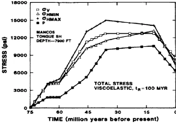
more detailed viscoelastic calculations. Figure 2.4 shows the viscoelastic behavior for
12
Figure 2.4: Viscoelastic behavior for a time of 100 million years in the Piceance basin. From Warpinski (1989).
13
2.4 Effects of Reservoir Depletion
It is important to address the problems associated with changes of effective
stress within and surrounding depleting reservoirs. Hydraulic fracturing can be just as
effective in depleted reservoirs as in the same reservoir prior to depletion because the
horizontal stresses will change during oil production. Equation 2.1 shows the
effective stress equations; it’s clear how the effective stress changes in depleting
reservoirs when the pore pressure reduced. In some weak reservoirs, compaction
drive is an effective mechanism for enhancing the total amount of hydrocarbons
recovered, especially if the permeability changes accompanying compaction are not
severe (Zoback, 2007).
σeff = σ1− αPpore (2.1) Where,
σeff = effective stress, psi σ1 = overburden stress, psi α = Biot’s constant Ppore = pore pressure, psi
There is an advantage of hydraulic fracturing a depleted reservoir which when
significant rotation of the principal stress direction occurs. If hydraulic fracturing was
used when wells were initially drilled in a tight reservoir, rotation of principal stress
directions during depletion would cause any new fracture to propagate at a new
14
Some studies (Al-Harthy et al, 1998) show the effect of the pore pressure
changes under various stress conditions. Pores are always subjected to two kinds of
stresses; one caused by fluid pressure inside the pores, the other one is caused by the
result of the surrounding formations. In their study, Al-Harthy et al (1998) focused on
the impact of dynamic permeability changes on the reservoir performance during the
production life, in other words, how the permeability changes with reservoir
depletion. The various loading paths used in these experiments affected the
permeability results. Figure 2.5 shows how the permeability is affected by pore
pressure under different stress paths. Our intent in this project relates to these
permeability results since the intent in this thesis is to explore how loading paths and
other laboratory variables can affect our laboratory results.
2.5 Brief Summary of Previous Project Works
The hydraulic fracture height growth and containment mechanisms project
conducted by the FAST Consortium is focused at gaining a better understanding of
fracture growth in laminated rocks. Casas (2005) performed a hydraulic fracturing
test on a Colton Sandstone block of high modulus and low permeability (Figure 2.6).
The focus of the experiment was to assess the effect of discontinuities on hydraulic
fractures.
Fluid lag zones (possibly due to dilatancy at the fracture tip) effectively shield
fluid pressure from the fracture tip, causing fluid net pressure inside the fracture to
increase, and fracture growth rate to significantly decrease. Hence, influence of the
15
becomes more related to hydraulic loading. The fracture growth behavior was
modeled and experimentally determined. Fluid lag and dilatancy behavior were seen
in the pressure profiles. The controlled laboratory experiments showed planar fracture
trends as expected from 3D modeling.
Figure 2.5: Effect of pore pressure on permeability under different stress-paths. From Al-Harthy et al. (1998).
16
Figure 2.6: Top view of Colton sandstone test block with layout of fabricated joints bonded with grout and epoxy. From Casas (2005).
The second phase of the project was performed by Athavale (2007). His work
focused on laboratory examination and finite element modeling to evaluate the effects
of layering, bedding and other factors as a hydraulic fracture intersects these features
in thin-bedded rocks. This project produced five blocks with layers of Lyons
sandstone and cement of differing mechanical properties using different bonding
agents at the layer interfaces (Figure 2.7). Conclusions from this project included
finite element modeling that shows that a triaxially loaded small laminated block with
layers having contrasting material properties experiences boundary effects in terms of
stress concentrations. In laboratory tests, fracture growth would be affected in terms
of width, pressures and shape due to the stress concentrations when the fracture
reaches these boundaries. Researchers need to be aware and take into consideration
these boundary effects while designing, interpreting and modeling these hydraulic
EPOXY GROUT
17
fractures. In subsurface formations, these boundary effects would not exist
considering the large aerial extent of the reservoir, and based on the experiments and
modeling conducted as part of this research, a combined effect of rock mechanical
property contrasts and in-situ stress contrasts appears to account for the complex
fracture growth in thinly laminated reservoirs.
Figure 2.7: Laminated blocks with different bonded interfaces. From Athavale (2007).
The third phase of the project is currently ongoing and is intended to extend
the former results to utilizing acoustic measurements as an independent diagnostic for
the dynamic fracture behavior. The use of small scale microseismic recordings and
analysis is the best mechanism to monitor and understand the dynamic behavior of
18
one synthetic cement block and one block of homogenous sandstone was conducted
to calibrate the system and experiment prior to running the tests on the synthetic
layered blocks (Figure 2.8).
Figure 2.8: Three-layer block preparation for acoustic sensors for the synthetic layered block in Phase 3. The top and bottom portions of the block consisted of cement, while the center portion was Lyons sandstone.
19
CHAPTER 3: FINITE ELEMENT METHOD
This chapter gives a brief history and a brief introduction to basic finite
element theory, discusses the equations used by the finite element modeling software
for solving structural mechanics problems, and the future of this method in general.
3.1 A Brief History of the Method
Although the finite element method first appeared in 1960, when it was used
by Clough in a paper on plane elasticity problems, the ideas for finites element
analysis date back much farther. The first efforts to use piecewise continuous
functions defined over triangular domains appear in applied mathematics literature
with the work of Courant in 1943. In 1959, Greenstadt outlined a discretization
approach involving cells instead of points; he imagined the solution domain to be
divided into a set of contiguous subdomains (Huebner et al, 2001).
As the popularity of the finite element method began to grow in the
engineering and physics communities, more applied mathematicians became
interested in giving the method for a firm mathematical foundation. Since the late
1960’s, the mathematical literature on the finite element method has grown more than
in any previous period (Huebner et al, 2001).
3.2 The Finite Element Method
The finite element method (FEM) (sometimes referred to as finite element
20
solutions of boundary value practical engineering problems. Simply stated, a
boundary value problem is a mathematical problem in which one or more dependant
variables must satisfy a differential equation everywhere within the known domain of
independent variables and also satisfy specific conditions on the boundary of the
domain. A boundary value problem is sometimes referred to as a field problem, and
the dependant variables of interest are referred to as field variables (Hutton, 2004).
In FEM, the physical domain or the structure is divided into several elements,
which are generally geometric shapes such as squares, triangles, quadrilaterals,
tetrahedrons, etc. The process of representing a physical domain with finite elements
is referred to as “meshing” and the resulting set of elements is known as the finite
element mesh. The mesh size influences the accuracy of the solution in terms of the
converging of the finite element solution to the exact solution of the problem. Such a
situation is shown in Figure 3.1a, where a curved boundary domain is meshed
coarsely using square elements. A refined mesh for the same domain is shown in
Figure 3.1b, using smaller, more numerous elements of the same shape. Note that the
refined mesh includes significantly more of the physical domain in the finite element
representation and the curved boundaries are more closely approximated.
Then the finite elements will be reconnected at nodes (vertices for shapes like
triangles, squares, etc.) which are the points at which the value of the field variable is
to be explicitly calculated. The solution for the problem consists of obtaining values
of a field variable at the finite element nodes by solving a set of governing equations.
21
connect an element to the adjacent finite elements. Interior nodes do not lie on
element boundaries and cannot be connected to any other element (Figure 3.2).
Figure 3.1: (a) Arbitrary curved boundary domain modeled using square elements. Grey areas are not included in the model. (b) Refined finite element mesh showing reduction of the area not included in the model on the left. From Hutton (2004).
Figure 3.2: (a) A general tow-dimensional domain of field variable. (b) A three-node finite element defined in the domain. (c) Additional element showing a partial finite element meshes of the domain. From Hutton (2004).
22
3.3 Some Methods for Solving Engineering Problems
There are a number of approaches to the solution of linear and non-linear
boundary value problems ranging from completely analytical to completely numerical
as follow:
I. Direct Integration
Separation of Variables
Similarity Solutions
Fourier and Laplace Transforms
II. Approximate Solutions
Perturbation
Power Series
Probability Series
Method of Weighted Residuals (MWR)
Ritz Method
Finite Difference Techniques
Finite Element Method
For a few problems, it is possible to obtain an exact solution by direct
integration of the differential equation. This is sometimes accomplished by an
obvious separation of variables or by applying a transformation that makes the
23
transformation of a differential equation leads to an exact solution (Huebner et al,
2001).
The Ritz method and the method of weighted residuals (MWR) are the two
methods commonly used as general solution methods for obtaining approximate
solutions to boundary value problems. The Ritz method has been used to derive the
equations of the FEM to find solutions to variational problems. However, in many
practical problems, the classical variational principles are unknown and hence the
(MWR) is used in a vast majority of applications where FEM is the numerical
technique of choice for being a more generalized procedure (Huebner et al, 2001).
The MWR is an approximate technique for solving the partial differential
equations. It uses trial functions that satisfy the prescribed boundary conditions and
an integral formulation to minimize error over the model domain. The method is
implemented as follows (Hutton, 2004)
Given a differential equation of the general form (Equation 3.1),
𝐷 𝑦 𝑥 , 𝑥 = 0 a < x < b (3.1)
Subject to homogeneous boundary conditions (Equation 3.2),
𝑦 𝑎 = 𝑦 𝑏 = 0 (3.2)
the method of weighted residuals seeks an approximate solution in the form
24 𝑦∗ 𝑥 = 𝑐
𝑖𝑁𝑖 𝑥 𝑛
𝑖=1 (3.3)
where y* is the approximate solution expressed as a product of ci unknowns,
constant parameters to be determined and Ni(x) trial functions. Equation 3.3 does not
give an exact solution. Instead, on substitution of the assumed solution into the
differential Equation 3.1, a residual error results such that:
𝑅 𝑥 = 𝐷[𝑦∗ 𝑥 , 𝑥] ≠ 0 (3.4)
where R(x) is the residual which is also a function of ci in Equation 3.3. The
MWR requires that the unknown parameter ci be evaluated such that:
𝑤𝑎𝑏 𝑖 𝑥 𝑅 𝑥 𝑑𝑥 = 0 i = 1 , n (3.5)
where wi (x) represents n arbitrary weighting functions.
Several variations of the MWR exist, and the techniques vary primarily in
how the weighting factors are selected or determined. The most common techniques
used are point collocation, subdomain collocation, least squares and Galerkins
method. Because of its simplicity and adaptability to the finite element modeling, the
25
In this method, the weighting functions are chosen to be identical to the trial
functions, that is (Equation 3.6),
𝑤𝑖 𝑥 = 𝑁𝑖(𝑥) i = 1 , n (3.6)
Therefore the unknown parameters are determined using Equation 3.7:
𝑤𝑎𝑏 𝑖 𝑥 𝑅 𝑥 𝑑𝑥 = 𝑁𝑎𝑏 𝑖 𝑥 𝑅 𝑥 𝑑𝑥 = 0 i = 1 , n (3.7)
resulting in n algebraic equations for evaluation of the unknown parameters.
3.4 A General Procedure for Finite Element Analysis
Certain steps in formulating a finite element analysis of a physical problem
are common to all such analyses, whether structural, heat transfer, fluid flow, or some
other problem. The steps are described in Sections 3.4.1 – 3.4.3:
3.4.1 Preprocessing
The preprocessing step is described as defining the model and includes these
components:
Define the geometric domain of the problem;
Define the element types to be used;
Define the material properties of the elements;
26
Define the element connectivities (mesh the model);
Define the physical constraints (boundary conditions); and,
Define the loadings.
3.4.2 Solution
During the solution phase, finite element software assembles the governing
algebraic equations in matrix form and computes the unknown values of the primary
field variables. The computed values are then used by back substitution to compute
additional, derived variables, such as reaction forces, element stresses, and heat flow.
It is not uncommon for a finite element model to be represented by tens of
thousands of equations. Special solution techniques are used to reduce data storage
requirements and computation time.
3.4.3 Postprocessing
Analysis and evaluation of the solution results is referred to as postprocessing.
Postprocessor software contains sophisticated routines used for sorting, printing, and
plotting selected results from a finite element solution. Examples of operations that
can be accomplished include:
Sort element stresses in order of magnitude;
Check equilibrium;
Calculate factors of safety;
Plot deformed structural shape; and,
27
While solution data can be manipulated many ways in postprocessing, the
most important objective is to apply sound engineering judgment in determining
whether the solution results are physically reasonable (Hutton, 2004). Chapter 4
shows the finite element modeling software used in this study and also the cases study
that have been run.
3.5 The Future of this Method
The finite element method, like any other numerical analysis technique, can
be made more efficient and easier to use. As the method is applied to larger and more
complex problems, it becomes increasingly important that the solution process remain
economical.
“Since mid 1970s interactive finite element programs on small but powerful personal computers and workstations have played a major role in the remarkable
growth of computer-aided design. This methodology is still exciting and important part of an engineering’s tool kit (Huebner et al., 2001).”
28
CHAPTER 4: FINITE ELEMENT MODELING
The main objective of this study is to evaluate the effect of stresses loading on
fracture growth in the laboratory and how to best apply these results to in-situ
formations. As showed before in previous work of Athavale (2007) in Chapter 2,
laboratory scaled hydraulic fracturing tests performed on a small sized cement block
showed that penny shaped fracture growth occurs when fractures are propagated
through an isotropic homogeneous medium. On the other hand, it was seen that
complex fracture growth occurs when the system is laminated with layers having
different material properties.
In an effort to model and study this stress-loading, Finite Element Modeling
(FEM) was performed on isotropic (one-layer), three-layer, and seven-layer systems.
This chapter describes the modeling software and the various inputs and control
functions.
4.1 Modeling Software
The finite element modeling software called COMSOL Multiphysics TM
(formerly FEMLAB) Version 3.5a was used in this study to model the three different
stressed blocks problems. COMSOL Multiphysics 3.5a is a powerful interactive
environment for modeling all kinds of scientific and engineering problems based on
partial differential equations. It contains built-in physics modes which can be used to
29
compiles a set of partial differential equations representing the entire model and
solves them using the finite element method. Partial differential equations can be
described through different mathematical application modes and using these
application modes, one can perform various types of analysis including stationary or
time dependant analysis, linear and non-linear analysis or Eigenfrequency and modal
analysis. Another useful feature of COMSOL Multiphysics 3.5a is that one can easily
extend conventional models for one type of physics into multiphysics models to solve
coupled physics phenomenon simultaneously. COMSOL Multiphysics 3.5a allows for
entering coupled systems of partial differential equations. The partial differential equations can be entered directly or using the so called “weak form”, which is a solution to an ordinary or partial differential equation which is a function for which
the derivatives appearing in the equation may not all exist but which is nonetheless
deemed to satisfy the equation in some precisely defined sense. It has a
Windows-based user friendly environment to work in and a very flexible and descriptive
graphical user interface (GUI). Using this software made it easy to model the stress
physics of the problem in question, and the analysis and visualization techniques were
useful to describe the solution outputs.
4.2 Block FE Modeling
This section describes defining the physics of the various block models in
COMSOL Multiphysics 3.5a, constructing the model, the input parameters and
30
methodology for performing the finite element modeling study is given in the flow
chart shown in Figure 4.1.
Figure 4.1: Flow chart for the finite element modeling using COMSOL Multiphysics 3.5a software. Define Geometry Postprocessing Set Material Properties Set Boundary Conditions Meshing Set the Solver
31
4.2.1 Geometry
To initiate the study, seven basic block systems were created and included a
single layer, homogeneous system, with and without a wellbore, as a control case; a
three-model layer with and without a wellbore; and three model blocks for seven layers (to coincide with Athavale’s (2007) work) with and without a wellbore and a wellbore with steel casing. For three-layer and seven-layer models, a composite
geometry object was created by joining together the layers. These base models were
built using the Structural Mechanics module and can simulate the laboratory
conditions during previous tests.
4.2.1.1 One-Layer Block Model
For the single layer model, the following parameters were used:
1 layer block dimensions: x = 11 in, y = 11 in, z = 15 in
Wellbore properties: r = 0.75 in and length = 15 in.
A schematic of this single-layer block is shown in Figure 4.2.
4.2.1.2 Three-Layer Block Model
For the three-layer system, the following properties were used:
3 layers block dimensions: x = 11 in, y = 11 in,
32
These z-direction dimensions were chosen because there are three different
layers composed of Lyon sandstone and cement 15.8 ppg in some of the performed
laboratory experiments (Figure 4.5).
The wellbore properties: r = 0. 5 in and length = 8.81 in from the top of the
block.
A schematic of this is shown in Figure 4.3.
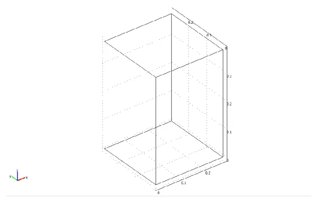
Figure 4.2: Model geometry for one-layer block without a wellbore from COMSOL Multiphysics 3.5a.
33
Figure 4.3: Model geometry for the three-layer block with a wellbore from COMSOL Multiphysics 3.5a.
4.2.1.3 Seven-Layer Block Model
The seven-layer model used the following parameters:
7 layers block dimensions: x = 11 in, y = 11 in,
z1 = 1.2 in, z2 = 1.0 in, z3 = 2.9 in, z4 = 2.9 in,
z5 = 2.9 in, z6 = 2.5 in, z7 = 1.6 in; these z-directions dimensions were
chosen because there are seven different layers which are Lyon sandstone, cement
15.8 ppg, cement 16.2 ppg, and the epoxy in Athavale’s 2007 work (Figure 4.6).
34
The casing thickness in Figure 4.4 is 0.11 in. The area between the top and
bottom casing stubs was openhole, which is where the fractures were initiated.
Figure 4.4: Model geometry for 7 layers block with a wellbore and the casing from COMSOL Multiphysics 3.5a.
4.2.2 Material Properties
The material property for the single layer block of Lyons sandstone was input
into the model. The material properties for the three-layer block of Lyons sandstone
and 15.8 ppg cement were input into the model. The material properties for the
seven-layer block of Lyons sandstone, 15.8 ppg cement, 16.2 ppg cement seven-layer and the
epoxy were input into the model. Figures 4.5 and 4.6 show the block construction for
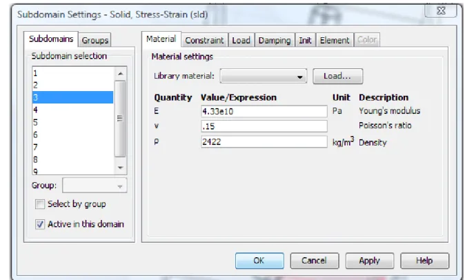
35
solve the problem, the software requires the material properties of Young’s modulus, Poisson’s ratio and density to be input for every material.
Table 4.1 shows the material properties for all block models used as input
data. For the sleeves used in the wellbore construction, a standard AISI 4340 steel
was selected from an in-built library of materials which the software provides.
Table 4.1: Input Data, the Material Properties for All Block Models Material Properties
Lyons
Sandstone
Poisson’s ratio (υ) = 0.15 Young’s modulus (E) = 6,280,134 psi Density (ρ) = 24.3 ppg Epoxy υ = 0.40 E = 440,914 psi ρ = 17.5 ppg Cement 15.8 ppg υ = 0.23 E = 1,290,835 psi ρ = 17 ppg Cement 16.2 ppg υ = 0.30 E = 2,204,573 psi ρ = 18 ppg
36
Figure 4.5: Three-layer block model constructed with alternate layers of cement and sandstone.
37
Figure 4.6: Seven-layer block model constructed with alternate layers of cement and sandstone.
38
Figure 4.7 shows the user interface from COMSOL Multiphysics TM for
inputting the material properties.
Figure 4.7: Window for inputting material properties for different layers in the seven-layer block model from COMSOL Multiphysics 3.5a. The subdomain value on the left controls what part of the model that the various parameters are assigned to during the modeling process.
4.2.3 Boundary Conditions
Table 4.2 shows the different boundary condition cases that have been used in
39
1. All faces of a block model are constrained except the top of the block, with
4200 psi applied as an overburden stress. The intent of this case is to calculate the
second and third principal stresses (σ2 and σ3) and verify the model with analytical
solutions.
2. This case represents 3D stresses that are not equal, i.e. σ1 ≠ σ2 ≠ σ3. Stress is applied on one face of each of the three directions, while the other faces are
constrained.
3. This is the same as Case #1 except the bottom face is not constrained. This
allows observation of how unconstrained boundary conditions affect the results.
4. The same as Case #1 but there are no constrained faces. Again, the intent is to
see how this affects the results such as the principal stresses or displacements values.
5. In this case, 4200 psi stress is applied on the top and the bottom of the block.
The rest of the faces are constrained.
6. This case represents 3D stresses that are not equal, i.e. σ1 ≠ σ2 ≠ σ3, and mimics the actual lab work that has been done.
7. All faces of the block models are constrained except the top of the block, with
4200 psi applied as an overburden stress. The stresses in this case applied gradually
from 0 psi to 4200 psi as an overburden stress (time-dependent feature).
8. This case represents 3D stresses that are not equal, i.e. σ1 ≠ σ2 ≠ σ3, mimicing
the actual lab work that has been done. The stresses in this case are applied gradually
from 0 psi to 4200 psi and the overburden stress is 4200 psi, 2700 psi is the maximum
horizontal principal stress and 1700 psi is the minimum horizontal principal stress. It
40
Table 4.2: Matrix of Cases Run and the Stresses Applied
Cases 1 layer 3 layers 7 layers
No well W/ well No well W/well No well W/ well W/well W/csg σov=4200 psi σH=σh=0 psi (1) All faces constrained - except the top - no horizontal pressures applied (2) Three faces constrained with 3 different stresses σov=4200 psi σH=2700 psi σh =1700 psi
(3) Four faces constrained – except top & bottom- with vertical stress
σov=4200 psi σH=σh=0 psi
(4) No face constrained – and just vertical stress
σov=4200 psi σH=σh=0 psi σov σov σh σH σov σov
X
X
X
X
X
X
X
X
X
X
X
X
X
X
X
X
X
X
X
X
X
X
X
X
X
X
X
X
41
(5) Apply pressure on the top and bottom “same value” – Four faces are constrained
σtop=σbottom =4200 psi
(6) Stresses applied on all faces - except the bottom. σov=4200 psi σH=2700 psi σh=1700 psi (7) Time-dependent , for Case # 1 σov=4200 psi σH=σh=0 psi (8) Time-dependent, for Case #6 σov=4200 psi σH=2700 psi σh=1700 psi
Table 4.2: Matrix of Cases Run and the Stresses Applied (continued)
σbott om σto p σov σH σH σh σh σov σov σH σH σh σh
X
X
X
X
X
X
X
X
X
X
X
X
X
X
X
X
X
X
X
X
X
42
Cases 3 – 5 were conducted just to understand the software behavior when the
stresses are applied in different situations. Cases 1 – 6 have been run as static;
however, time plays an important role to simulate the experiments in laboratory work
when the stresses are applied. For example, when stresses were applied in the lab on
the actual blocks it takes approximately 30 minutes to reach the maximum target
stress of 4200 psi. These stresses are not applied instantaneous. Figure 4.8 shows how
the stress changes with time in a simulation model for Cases 7 and 8. Figure 4.9
shows the user interface from COMSOL Multiphysics 3.5a for inputting the stresses
changing with time for the model. To define functions based on interpolated data, we
used the “Functions” dialog box shown in Figure 4.9. A new interpolation function
was defined and the stress data were entered.
Figure 4.10 shows an example of the user interface from COMSOL
Multiphysics 3.5a for inputting boundary conditions for the model. For the triaxially
stressed laminated block shown in this example, the boundary conditions, which were
used for the actual laboratory experiments, were imposed to analyze stresses and
displacements:
A stress of 1700 psi (minimum horizontal principal stress) was applied to the block face in the y-direction. The boundaries were not constrained
and were free to move.
A stress of 2700 psi (maximum horizontal principal stress) was applied at the block face in the x-direction. The boundaries were not constrained
43
Figure 4.8: The applied stress changes with time (30 minutes). All three directional stresses are increased until the overburden stress reach 4200 psi, the maximum horizontal principal stress reach 2700 psi, and the minimum horizontal principal stress reaches 1700 psi.
44
Figure 4.9: Windows in COMSOL Multiphysics 3.5a for inputting the time function for the time-dependent problems. x stands for the maximum horizontal principal stress, y for the minimum horizontal stress, and z for the overburden stress.
A stress of 4200 psi (overburden stress) was applied to the top face of the block. The top face was not constrained and was free to move.
No load was applied on the bottom face but it was constrained to move in the z-direction.
4.2.4 Meshing
The process of representing a physical domain with finite elements is called “meshing”. Since most of the commonly used mesh element geometries have straight edges, it is impossible to include the entire physical domain in the element mesh if
45
Figure 4.10: Data entry window in COMSOL Multiphysics 3.5a for inputting the boundary conditions for the problems. Constraint and load can be set for the different boundaries in the models.
In such a situation, where the physical domain is meshed rather coarsely,
mesh refinement is needed where smaller but more numerous elements of the same
type are used. A refined mesh includes significantly more of the physical domain in
the finite element representation and boundaries are more closely approximated. As
the number of elements is increased and the physical dimensions of the elements are
decreased, the finite element solution changes incrementally. The incremental
changes decrease with the mesh refinement process and approach or converge to the
exact solution asymptotically (Hutton, 2004). A refined mesh will more closely