Accessed drainage volume and recovery factors of fractured horizontal wells under transient flow

ACCESSED DRAINAGE VOLUME AND RECOVERY FACTORS OF FRACTURED HORIZONTAL WELLS UNDER TRANSIENT FLOW

by

ii

A thesis submitted to the Faculty and the Board of Trustees of the Colorado School of

Mines in partial fulfillment of the requirements for the degree of Master of Science

(Petroleum Engineering). Golden, Colorado Date: ______________________ Signed: ______________________ Caglar Yesiltepe Signed: ______________________ Dr. Erdal Ozkan Thesis Advisor Golden, Colorado Date: ______________________ Signed: ______________________ Dr. Erdal Ozkan

Professor, Petroleum Engineering

iii ABSTRACT

The objective of the research presented in this Master of Science thesis is to propose a

practical approach to estimate the drainage volume and recovery factors of fractured

horizontal wells in tight, unconventional reservoirs under economic constraints. For

conventional wells, economic depletion of a given drainage area is mainly dictated by

physical depletion. For fractured horizontal wells in unconventional reservoirs, however,

economic depletion rates are usually reached during transient flow and recovery factors are

insensitive to well spacing. A consequence of this phenomenon is the disparity of the

observed ultimate recovery from the estimates based on well-spacing considerations, which is

also manifested in the inconsistencies of the estimated recovery factors of wells in

unconventional reservoirs. Furthermore, economic depletion during transient flow also has

implications on more efficient utilization of unconventional hydrocarbon resources.

In this work, a contacted reservoir volume (CRV) is defined based on the effective

transient drainage area of the well under linear-flow conditions. This definition enables the

estimation of physically and economically meaningful recovery factors based on accessable

reserves of the well for an economic cut-off rate. Equations to estimate effective drainage

areas of fractured horizontal wells under linear and compound linear flow conditions are

derived and related to the CRV for a given transient production rate. This approach provides

a practical means of optimizing hydraulic fracture spacing along a horizontal well. Example

applications of the proposed approach are demonstrated and the results are discussed. The

work presented in this thesis does not consider the geomechanical changes caused by

iv

TABLE OF CONTENTS

ABSTRACT ... iii

LIST OF FIGURES ... vi

LIST OF TABLES ... viii

ACKNOWLEDGEMENTS... ix

CHAPTER 1 INTRODUCTION ... 1

1.1 Organization of the Thesis ... 2

1.2 Motivation of the Research ... 3

1.3 Statement of the Problem ... 6

CHAPTER 2 BACKGROUND ... 8

2.1 Decline Curve Analysis... 9

2.2 Physical Drainage Area and Transient Drainage Area ... 15

2.2.1 Drainage Areas of Horizontal and Fractured Wells ... 16

2.2.2 Radius of Investigation ... 20

2.2.3 Transient Drainage Radius ... 23

2.3 Optimum Well Spacing ... 24

2.4 Isochronal Testing ... 29

2.5 Trilinear Flow Model for Fractured Horizontal Wells ... 34

CHAPTER 3 TRANSIENT DRAINAGE AREAS OF FRACTURED HORIZONTAL WELLS ... 40

3.1 Transient Drainage Areas of Fractured Horizontal Wells ... 40

3.1.1 Transient Drainage Areas of Horizontal Well Fractures ... 41

3.1.2 Transient Drainage Areas of Fractured Horizontal Wells ... 46

3.2 Verification of the Results ... 48

3.2.1 Time to Reach the Boundary Between Two Fractures ... 49

3.2.2 Verification With Trilinear Model Flow Regimes ... 53

v

4.1 Contacted Reservoir Volume (CRV) and Recovery Factor Calculations ... 58

4.1.1 Case 1: Hydraulic Fracture Spacing ... 59

4.1.2 Case 2: Horizontal Well Spacing ... 65

4.2 Economic Analyses ... 71

4.2.1 Case 1: Hydraulic Fracture Spacing ... 72

4.2.2 Case 2: Horizontal Well Spacing ... 73

CHAPTER 5 CONCLUSIONS ... 76

NOMENCLATURE ... 79

vi

LIST OF FIGURES

Figure 1.1 Well Spacing and drainage area considerations for conventional wells. ... 4

Figure 1.2 Production decline and cumulative production at a cut-off rate for a vertical well in a conventional reservoir. ... 4

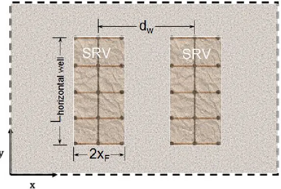
Figure 1.3 Schematic of two fractured horizontal wells surrounded by stimulated

reservoir volumes (SRV) in an unconventional reservoir. ... 5

Figure 1.4 Demonstration of production decline and cut-off rate for a fractured

horizontal well in an unconventional reservoir. ... 6

Figure 2.1 Arps’ (1945) decline curves. ... 11

Figure 2.2 El-Banbi and Wattenbarger Method, 160 Acres Linear Flow

(Cox et al. 2005). ... 17

Figure 2.3 Rate Cumulative Decline Method, 160 Acres Linear Flow (Cox et al. 2005). 18

Figure 2.4 Flow-after-flow test sequence. ... 31

Figure 2.5 Flow-after-flow test analysis: A. Analytical approach using Eq. 2.37 and B. Empirical approach of Rawlins and Schellhardt (1936) using Eq. 2.41. .... 31

Figure 2.6 Isochronal test sequence. ... 33

Figure 2.7 Isochronal test analysis: A. Analytical approach using Eq. 2.37 and

B. Empirical approach of Rawlins and Schellhardt (1936) using Eq. 2.41. .... 33

Figure 2.8 Schematic of the trilinear flow model representing three contiguous flow regions for a multiply fractured horizontal well (Brown et al., 2009). ... 35

Figure 3.1 Schematic representation of the trilinear flow idealization of the fractured horizontal well consider in this chapter. ... 41

Figure 3.2 Schematic representation of y for the inner reservoir in trilinear flow _i

model. ... 41

Figure 3.3 Schematic representation of x . ... 47 _i

Figure 3.4 Schematic representation of two fractured horizontal wells surrounded by stimulated reservoir volumes (SRV). ... 48

Figure 3.5 Schematic (areal) representation of 1D linear flow toward a fractured well in a slab reservoir. ... 50

vii

Figure 3.6 2

. D dD

t vs y satisfying Eq. 3.39. ... 53

Figure 3.7 Stabilization time and the effect of the outer reservoir for the homogeneous inner reservoir case. ... 56

Figure 3.8 Stabilization time and the effect of the outer reservoir for the dual-porosity inner reservoir case





Figure 4.1 q vs. t for Case 1. ... 59

Figure 4.2 q vs. y for Case 1. ... 60 _i Figure 4.3 y corresponding to a cut-off rate in Case 1. ... 60 _i Figure 4.4 RF vs. t for Case 1. ... 63

Figure 4.5 Transient RF vs. t based on CRV for Case 1. ... 64

Figure 4.6 Contribution of the outer reservoir for different x values in Case 2. ... 66 _e Figure 4.7 q vs. t for Case 2 (p_wf 500psi and x _e 10, 000ft)... 66

Figure 4.8 q vs. t for Case 2 in larger scale (p_wf 500psi and x _e 10, 000ft) ... 67

Figure 4.9 RF vs. t for Case 2. ... 70

Figure 4.10 Transient RF vs. t for Case 2. ... 70

Figure 4.11 NPV vs. t for Case 1. ... 72

Figure 4.12 NPV vs. n for Case 1. ... 73 _F Figure 4.13 NPV vs. t for Case 2. ... 74

viii

LIST OF TABLES

ix

ACKNOWLEDGEMENTS

Firstly, I would like to express my appreciation and gratitude to my advisor Dr. Erdal

Ozkan, for his guidance, help and support throughout my research and including me in his

consortium, Unconventional Reservoir Engineering Project (UREP). Thanks to his

knowledge, encouragement and patience, I learned a lot in my Master of Science study. I

would also like to thank my thesis committee members, Dr. Hulya Sarak, and Dr. Azra

Tutuncu for their times and suggestions. Dr. Hulya Sarak deserves special thanks for her

valuable help in my research. I would like to thank Denise Winn-Bower for her helps and

friendliness throughout my study at Colorado School of Mines. I would also like to thank to

faculty and staff in Petroleum Engineering Department of CSM.

I would like to acknowledge The Turkish Petroleum Corporation (TPAO) for

sponsoring my MSc study.

I would like to thank all my friends in Golden. I had great memories and experiences

in two and a half years. Special thanks to Hakan Corapcioglu, Mehmet Hazar, Ozlem Ozcan

and Sarp Ozkan for their help and support.

Finally, I am grateful to my father Dr. Ridvan Yesiltepe, my mother Gulten Yesiltepe

and my sister Ceren Yesiltepe for always being there for me and supporting me even if they

are many miles away. I would also like to thank my girlfriend (future wife) Fulden Ozkoldas

1 CHAPTER 1

INTRODUCTION

Hydrocarbon accumulations that cannot be characterized and produced with the

existing conventional procedures and technologies are considered as unconventional

reservoirs. Unconventional reservoirs can also be identified based on their complex

geological, geochemical, and petrophysical properties, heterogeneities at all scales, and

unusual flow mechanisms contributing production. Coalbed methane reservoirs, shale gas,

tight gas sands, and tight/shale oil reservoirs are examples of unconventional reservoirs that

have significantly climbed up the ladder in contributing to the energy supply of the US during

the past decade and they have attracted even more attention worldwide.

The focus of this research is the recovery factors of wells in shale-gas and tight-oil

plays. Due to the ultra-low permeabilities (in the nano-Darcy range) of these plays, attaining

economic production rates requires expensive well construction, stimulation, and production

technologies. Horizontal wells stimulated with multi-stage hydraulic fractures are the proven

technology to develop the shale-gas and tight-oil plays in the US (Ilk et al., 2011).

Unfortunately, the methods used to predict the ultimate recovery and long-term project

economics of these complex systems have originated from the conventional reservoir

development practices and are not reliable, if not completely inapplicable, for unconventional

reservoirs.

In this work, an effective drainage volume will be defined and used to introduce the

concept of contacted reservoir volume (CRV) of a fractured horizontal well. These concepts

will be extended to the estimation of the ultimate recovery and recovery factor under given

2 1.1 Organization of the Thesis

In this first chapter, the motivation and the objectives of the thesis are explained.

Chapter 1 also presents the research methodology, the structure of the thesis.

In Chapter 2, a review of the relevant literature and discussion of the some

fundamental concepts used in this research are presented. The discussion of production

decline analysis and the review of the theory of isochronal testing set the stage for the

development of the contacted reservoir volume concept and the recovery factor estimation

approach proposed in this research. Although the methodology used in this work is general,

the derivation of the particular equations and the examples provided assume the dominance

of linear flow regimes for fractured horizontal wells in tight reservoirs. A brief introduction

of the trilinear flow model used in the developments is also given in Chapter 2.

The derivation of the central results of this work is provided in Chapter 3. The

analytical derivation of the effective drainage area as a function of time and the expression of

the contacted reservoir volume for a limiting (economic) rate are presented in this chapter.

Chapter 3 also presents verification of the expressions derived in this work.

Example applications of the concepts and tools developed in Chapter 3 are given in

Chapter 4. The results are discussed and the differences from conventional interpretations are

highlighted in this chapter.

Finally, Chapter 5 provides the conclusions of the study including some suggestions

3 1.2 Motivation of the Research

Unconventional reservoirs, especially shale-gas and tight-oil plays, which are the

focus of this research, have ultra-low permeabilities (in the nano-Darcy range) that require

expensive well construction, stimulation, and production technologies to achieve economic

production rates. The common and proven well completion practice in the US

unconventional plays has been horizontal wells with multi-stage hydraulic fracturing (Ilk et

al., 2011).

Horizontal well spacing, number of hydraulic fracture stages along the well, and the

recovery factors are some of the key parameters influencing the economic success of an

unconventional-play development. Unfortunately, the methods to estimate these parameters

have originated from the conventional reservoir development practices and are not reliable, if

not completely inapplicable, for unconventional reservoirs. A consequence of this

phenomenon is the disparity of the observed ultimate recovery from the estimates based on

well-spacing considerations, which is also manifested in the inconsistencies of the estimated

recovery factors of wells in unconventional reservoirs.

Well spacing has always been an important problem for the oil and gas industry

(Aminian et al., 1985). According to Roberts (1961), optimum well spacing determined by an

economic analysis usually dictates drainage areas less than the maximum physical drainage

area of the well. It is known that productivity is inversely proportional to well spacing (Figure

1.1). Drilling additional wells will increase the productivity of each well, because tighter well

spacing accelerates the recovery of reserves, which is favored by project economics.

However, it will also increase the drilling costs. For this reason, Net Present Value (NPV)

4

Figure 1.1 Well-spacing and drainage area considerations for conventional wells.

Most conventional wells reach an economic cut-off rate during boundary-dominated

flow. At the cut-off rate, the drainage area is very close to physical depletion (Figure 1.2).

Therefore, if the productivity or ultimate recovery is calculated by using the economic cut-off

rate, it will be approximately equal to that calculated by using physical depletion. As a result,

for conventional wells, physical depletion can be used as a basis for recovery factors and

project economics.

Figure 1.2 Production decline and cumulative production at a cut-off rate for a vertical well in a conventional reservoir.

Similar to conventional wells, well spacing is one of the most important factors

affecting the economics of unconventional reservoir development projects. It is usually

assumed that the physical drainage area of fractured horizontal wells is a function of the well

5

the efficiency of the depletion of the reservoir between fractures (SRV) depends on the

efficiency of the stimulation, which is, in turn, a function of the number of fractures along the

well. In other words, the number of fractures affects the recovery from the reservoir volume

between fractures. On the other hand, to increase the recovery efficiency of the volume

between the two SRVs in Figure1.3, either the lengths of the hydraulic fractures, 2x_F, should be increased or the distance between two horizontal wells, d_w, should be decreased.

Figure 1.3 Schematic of two fractured horizontal wells surrounded by stimulated reservoir volumes (SRV) in an unconventional reservoir.

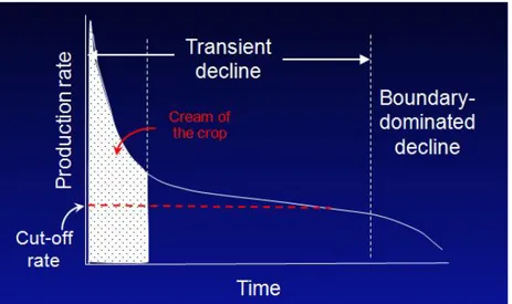
Most fractured horizontal wells in unconventional reservoirs, on the other hand, reach

an economic cut-off rate during transient flow (Figure 1.4); that is, the project economics is

mostly dictated by economic depletion. Therefore, an approach to directly relate recovery to

6

Figure 1.4 Demonstration of production decline and cut-off rate for a fractured horizontal well in an unconventional reservoir.

1.3 Statement of the Problem

Estimating the ultimate recovery of a well is fundamentally a material balance

application. Two essential elements of this material balance exercise are the drainage volume

of the well and the pressure or rate decline trend between the initial and final states.

Production data of most conventional wells display a well-defined decline trend after a short

transient flow period. The stabilized decline trend is a result of the boundary-dominated flow

within a fixed drainage volume defined by well spacing. For fractured horizontal wells in

unconventional reservoirs, on the other hand, the effective drainage area changes with time

and is not directly related to well spacing, flow is under transient conditions, and the decline

trend does not stabilize to perform material balance.

In this work, the potential disconnect between the well spacing and drainage area of

the well will be highlighted and its implications on common reserve estimation techniques

used in practice will be discussed. Then, an effective drainage area definition will be

7

horizontal well. These concepts will finally be extended to the estimation of recovery under

8 CHAPTER 2 BACKGROUND

As already noted in the Introduction (Chapter 1), either the conventional approaches

or some palliative modifications of them are used to estimate the reserves of unconventional

reservoirs. Therefore, to be able to appreciate the work done in this thesis research, a review

of the existing literature and critical discussion of the relevant concepts should be useful.

One of the fundamental techniques used for reserve estimation and performance

prediction in conventional and unconventional reservoirs is production decline analysis.

Because of the empirical nature of decline-curve analysis ideas, which stems from

observations of conventional vertical-well performance (Arps 1945), efforts to extend these

techniques to unconventional reservoirs should first critique the conditions of their

applicability.

Another related topic is the common practice (out of necessity) of the use of transient

production performance in the estimation of future production and ultimate recoveries.

Usually, ultimate recovery and recovery factor concepts are perceived to be associated with

the physical drainage of the reservoir, which requires the definition of the well’s drainage

area. If the pressure pulse due to production at the well location has not reached the physical

(or flow) boundary of the well (transient flow period), then the drainage area is not fixed. In

this thesis, the idea behind isochronal testing of production wells will be used to define

effective drainage areas of fractured horizontal wells in unconventional reservoirs during

transient flow. The discussion of isochronal testing will also be useful to highlight that, in the

absence of a reference point during the stabilized flow period (boundary dominated flow),

9

Finally, an overview of the trilinear flow model developed by Brown et al. (2009) will

be useful to explain the basis of the linear flow models used in the development of the results

presented in this thesis. As emphasized, earlier in the introduction, neither the trilinear flow

model nor the linear flow assumption is required for application of the general concepts and

methodology presented in this work. The trilinear flow model has been selected because of its

widespread use for fractured horizontal wells in unconventional reservoirs and analytical

convenience.

Before we start, it is also useful to note that the results of this work can be used for

single-phase oil and gas. For applications to gas wells, it is necessary to make some

simplifying assumptions that lead to the linearization of the gas-flow problem in porous

media in terms of a real-gas pseudopressure (Al-Hussainy et al., 1966):

( ) 2 b p p p p dp z   

_

where p is a reference pressure. The details and the assumptions of the pseudopressure _b

approach are given by Al-Hussainy et al. (1966) and will not be repeated here. Under the

pseudopressure approximation, we will use pressure and pseudopressure interchangeably in

this thesis. Also, in this work, we will assume that the variability of the

viscosity-compressibility product with pressure is negligible so that the discussion of the ideas such as

real-gas pseudotime (Agarwal, 1979) is not relevant.

2.1 Decline Curve Analysis

In most fields, production rate is regularly measured on daily or monthly basis.

Recently, for some wells, wellhead pressures are also measured and recorded regularly

together with production rates. Production data can be analyzed by decline-curve and p/z

10

transient flow conditions, rate-transient analysis (RTA) can also be used to estimate

formation properties and skin.

Since its proposal by Arps (1945), decline-curve analysis has received great

acceptance by the industry and become an industry standard for the prediction of future well

performances and ultimate recovery. The basis of the decline-curve analysis technique is the

following empirical equation proposed by Arps (1945) to describe natural production decline

of vertical wells in oil reservoirs under constant pressure production:





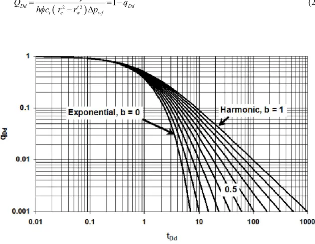
Arps (1945) described three types of decline behavior:

(i) b = 0 : Exponential decline (straight line on semi-log plot)

(ii) 0 < b < 1 : Hyperbolic decline (curved line on semi-log plot)

(iii) b =1 : Harmonic decline

The decline curves expressed by Eq. 2.2 are shown in Figure 2.1 in terms of

dimensionless flow rate and dimensionless time defined by

    ₃ 3 ln 4 7.08 10 e w Dd Dd i wf r q t r q t q x kh p           _         (2.3) and





11





exp w w

r r S (2.5)

and D is the decline rate defined by

D 1 dq q dt

  (2.6)

Based on the definitions of q_Dd and t_Dd in Eqs. 2.3 and 2.4, the dimensionless

cumulative production is given by (Raghavan, 1993)





Figure 2.1 Arps’ (1945) decline curves.

The analysis of production decline data consists of the following steps:

1. Rate versus time is plotted on a tracing paper with the same scale of the decline type

12

2. The tracing paper is moved on the type curve, keeping y and x axes parallel to the

respective axes of the type curve until a match is obtained with one of the curves.

3. Once the match is obtained, the value of b is directly read from the curve that is

matched with the field data

4. A match point is selected (any point can be used as a match point) and the match

point values of the dimensionless rate and time on the field plot and type curve are

recorded.

5. Values of qi and Di are calculated by using the match point values in the following

relations: i Dd match q q q        (2.8) and Dd i match t D t        (2.9)

Once qi and Di are known, Eq. 2.2 can be used to predict the future production.

Cumulative production, N_p, and remaining reserves, N , corresponding to a cut-off rate, _r q_co

, can be computed, respectively, from





13

In addition to its proven success, the popularity of decline-curve analysis can also be

attributed to its simplicity and the fact that production data is readily available for most wells.

Unfortunately, over the years, the assumptions and limitations of decline curve-analysis have

been overlooked and its applications have been extended to cases where it was not intended.

One of these cases is the analysis of production data from fractured horizontal wells in tight

unconventional reservoirs.

As mentioned above, the decline curve equation (Eq. 2.2) is an empirical relation and

its basis is Arps’ observations from oil fields of his time. The most important conditions of

Arps’ decline relations are

(i) Vertical well

(ii) Single-phase oil flow

(iii) Constant-pressure production

(iv) Stabilized (boundary-dominated) flow

In 1987, Fetkovich combined transient and boundary dominated flow periods to

construct more comprehensive decline type curves. Later, Palacio and Blasingame (1993) and

Agarwal et al. (1999) extended decline-curve analysis to gas flow under variable-rate and

variable-pressure production conditions and to fractured wells. These extensions addressed

the limitations of decline-curve analysis for items (i) through (iii) above. However, item (iv)

(boundary dominated flow) is an essential condition for decline curve analysis and cannot be

removed or replaced.

In principle, Arps’ decline curves assume a tank model (zero-order representation of

the well’s drainage volume) and apply material balance. Two essential elements of this

14

the initial and final states. Production data of most conventional wells display a consistent

and well-defined decline trend after a short transient flow period. For fractured horizontal

wells in unconventional reservoirs, on the other hand, flow is under transient conditions, and

there is no persistent decline trend applicable for the entire range of the production.

The brute-force application of decline curve analysis to fractured horizontal wells in

tight reservoirs yields b values larger than 1 (which is outside the range of b proposed by

Arps) and no single b value can represent the entire production data. Under these conditions,

extrapolation of Eq. 2.10 to infinity yields infinite cumulative production (Ilk et al., 2011)

indicating the problem with the material balance (as the drainage volume is not fixed during

transient flow).

Some new extensions of decline-curve analysis have also been proposed recently for

applications to shale-gas wells, such as (Lee and Sidle, 2010)

 Arps’ model with terminal minimum decline rate

 Stretched exponential decline model

 Long duration linear flow

 Duong’s decline model

 Analytical reservoir models

The detailed discussion and criticism of these ideas is outside the scope of the current

research. It suffices to note here that, none of these extensions have resolved the

inconsistencies in the application of decline curve analysis to fractured horizontal wells in

unconventional reservoirs; particularly, the issue about the drainage area changing with time

during transient flow has not been addressed in any of the above-mentioned extensions. We

15

resemblance to that encountered in isochronal testing, which will be discussed later in this

chapter for completeness.

2.2 Physical Drainage Area and Transient Drainage Area

Physical drainage area of a well is defined either by impermeable physical boundaries

or by no-flow boundaries imposed by the interference of nearby wells. During transient flow,

however, wells do not produce from the entire physical drainage area and the physical

drainage area does not influence flow and production characteristics. Two possible

interpretations of transient flow may be useful for our discussions in this work: at any time

during transient flow (i) the distance reached by the pressure pulse due to production at the

wellbore is smaller than the distance to the boundary of the drainage area, or (ii) production

at the wellbore consists of fluids withdrawn from a distance from the well which is less than

the distance to the drainage boundary.

As we discussed in the Introduction, it is not uncommon for unconventional wells to

reach the end of their economic life while still producing under transient flow conditions and

their physical drainage areas are immaterial for their performances. To apply the

conventional techniques of estimating ultimate recovery and recovery factors, it is useful to

define a transient drainage area that is smaller than the physical drainage area and a function

of time. The two interpretations of transient flow given above may be used to define the

transient drainage area: The first condition leads to the concept of radius of investigation and

the second condition yields the definition of effective transient drainage area. Before

discussing the concept of transient drainage during transient flow, we first cite the relevant

16

2.2.1 Drainage Areas of Horizontal and Fractured Wells

Definition of the drainage areas of horizontal wells requires different considerations

than those for vertical wells. Joshi (1990) introduced several geometric approaches to

calculate the drainage area of a horizontal well in isotropic and anisotropic reservoirs based

on the relationship between the drainage areas of a vertical well and that of a horizontal well.

He considered the effect of lateral anisotropy on the estimation of horizontal-well drainage

area.

In 1992, Reisz introduced a method to estimate the original oil in place, recoverable

reserves, and drainage area of a horizontal well in Bakken formation. Reisz’s method uses

material balance and decline curve analysis for single-phase flow. The weakness of this

method is to contain recovery factor in the drainage area equation. Recovery factor may be

unknown for many cases.

Later El-Banbi and Wattenbarger (1996) introduced a method, which couples the

material balance equation for gas reservoirs with the stabilized gas flow equation. During

boundary dominated flow, their iterative technique can be used to estimate the drainage

volume of the well. After that, results can be associated with the reservoir properties in the

volumetric equation to estimate the effective drainage area.

El-Banbi and Wattenbarger (1996) ignored non-Darcy flow and used the stabilized

flow equation for gas reservoirs given by

 





m p m p aq (2.12)

where a is a constant during stabilized (boundary-dominated) flow. Therefore, if,

 





m p m p q

  

17

flow. This plot requires that the initial gas in place be known to estimate the average pressure,

p , as a function of time.

El-Banbi and Wattenbarger suggested that an initial gas in place be assumed and

 

_

_

m p m p q

  

  is plotted versus time. If the in place volume is assumed too large, the

plot would have a positive slope at late times. If the assumed volume is too small, the slope

would be negative. The correct estimation of gas in place would give a zero slope at late

times provided that the well reaches stabilized flow. Cox et al. (2005) give an example

application of this technique for a single layer, 160-acres linear system (Figure 2.2).

Figure 2.2 El-Banbi and Wattenbarger Method, 160 Acres Linear Flow (Cox et al. 2005).

In 1998, Agarwal and Gardner introduced a new method to estimate effective

drainage area. In this method, rate-cumulative production-decline type curve is generated by

plotting reciprocal dimensionless wellbore pressure, 1 / p_wD, versus dimensionless cumulative

production, Q_DA, which are given, respectively, by

 

 

18

 

 

This plot forms a straight line tending towards Q_DA1 2





boundary-dominated flow provided that the average pressure, p , can be accurately estimated. After

stabilized flow is reached, the effective drainage area can be accurately calculated from this

method. Similar to the approach proposed by El-Banbi and Wattenbarger (1996), the

approach suggested by Agarwal and Gardner (1998) requires an iterative procedure on the

values of original gas in place to be used in the estimation of average pressure, p . When the

correct gas in place is guessed, the plot of 1 / p_wD versus Q_DA gives a straight line with the

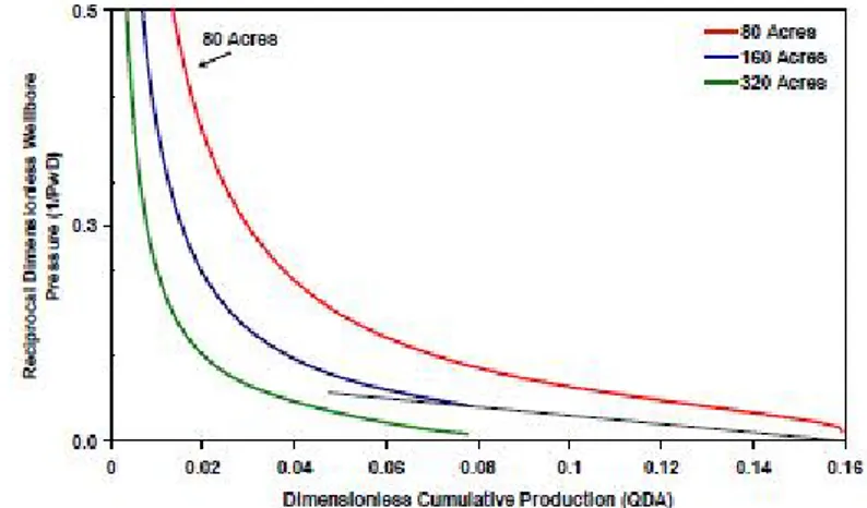
horizontal intercept of Q_DA 0.16. Figure 2.3 shows an example application of this procedure given by Cox et al. (2005) for a single layer, 160-acres linear system.

Figure 2.3 Rate Cumulative Decline Method, 160 Acres Linear Flow (Cox et al. 2005).

Later, Permadi et al. (2000) provided a method to estimate the drainage area of a

horizontal well. The method was developed by combining production decline equation with

material balance equation. They assumed production at a constant bottomhole pressure and

19

 

At pseudosteady-state, the productivity index of a horizontal well, J , is given by _h

(Joshi 1990) 0.00708 0.523 ln 0.75 2 h h e e e w k hL J Y h h B X Y h L r L       _   _     _{     }          (2.16)

The drainage area, A , can be calculated from Eq. 2.15, if production data and other

parameters are available. However, in some cases, production data may be unreliable. In such

cases, Permadi et al. suggest to use decline curve equation proposed by Shirman (1998) to

predict the decline trend. Shirman’s decline curve equation is given by

 

_

_

q t q baq t  (2.17)

Substituting Eq. 2.17 into Eq. 2.15 results in





Note that this equation also requires an iterative solution as the computation of J (Eq. 2.16)

requires the knowledge of the drainage area (A X Y_{e e}).

In 2005, by using El-Banbi-Wattenbarger and Rate Cumulative Decline Methods, Cox

et al. (2005) determined the drainage area for dry-gas reservoirs and highlighted the relative

importance of reservoir parameters, flow geometry, fracture half-length, and producing

20 2.2.2 Radius of Investigation

Radius of investigation is a concept used in pressure-transient analysis to indicate the

reservoir volume contacted during a well test in which the estimated properties should be

useful. Many definitions of radius of investigation are available in the literature. Because for

our purposes in this thesis, the choice of the radius of investigation has little or no impact on

our results, we will not delve into the nuances of various radius-of-investigation definitions.

Kuchuk (2009) provides a detailed discussion of the most used definitions and highlights the

fact that all these definitions are somewhat arbitrary as “there is no a definable radius of

investigation from pressure diffusion.” In this thesis, the definition of radius of investigation

from the analytical solution proposed by Lee (1982) will be used. However, the use of other

radius-of-investigation definitions would only lead to an adjustment of the coefficients in our

equations while the form of the equation and the qualitative discussions remaining

unchanged.

Lee (1982) defines the radius of investigation as “the distance of the maximum

pressure disturbance for an impulse source or sink”. Lee uses an analytical solution to define

radius of investigation by considering an injection well into which a volume of liquid is

injected instantaneously. This injection causes a pressure disturbance into the formation, and

at the time t the pressure disturbance at radius _m r reaches a maximum. To be able to obtain a _ı

relationship between r and _ı t , Lee used the solution of diffusivity equation for infinite _m

cylindrical reservoir with line-source well, given by

2 948 70.6 t i i c r qB p p E kh kt       _ _   (2.19)

where p is pressure (psi), t is time (hours), r is distance from the well at time t (ft), and Ei

21





_

From Eq. 2.19, the pressure variation at a time is given by

2_{/ 4} 1 r t c p e t t      (2.21)

where c is a constant, related to the strength of the instantaneous source. The time, ₁ t , at _m

which the pressure disturbance is a maximum at r is found by differentiating Eq. 2.21 and i setting equal to zero:

2 2 2 2 / 4 / 4 1 1 2 2 3 0 4 r t r t c c r p e e t t t            (2.22) Then, 2 2 948 4 i t i m r c r t k     (2.23)

So, at time t, a pressure disturbance reaches a distance r , which is called the radius of _i

investigation and given by

1/2 948 i t kt r c         (2.24)

As indicated by Eq. 2.24, the radius of investigation is directly proportional to

permeability and inversely proportional to porosity, viscosity, and total compressibility.

When the pressure pulse reaches the physical or flow boundary of the well, the radius of

investigation should be equal to the drainage area of the well. Therefore, if we take a

snapshot at a time, the radius of investigation may be interpreted as the effective drainage

22

Using the radius of investigation equation (Eq. 2.24), one can also find the duration of

time required for a pressure pulse created at the source location (well) to reach the boundaries

of the reservoir (time required to reach stabilized flow). If a well, which is centered in a

cylindrical reservoir of radius r , is assumed, setting _e r_i  yields the following expression r_e

for stabilization time:

2 948 _{t e} s c r t k   (2.25)

If we define a dimensionless time,

4 2.637 10 AD t kt t c A     (2.26)

where t is in hour and, for a circular drainage area, Ar_e2, Eq.2.26 yields

0.08 AD

t  (2.27)

which matches the time to reach pseudosteady state given by Earlougher (1977) and Larsen

(1983).

Building on the definition of Lee (1982), Datta-Gupta et al. (2011) introduced “the

depth of investigation” concept and generalized the radius of investigation concept to

heterogeneous conditions and more complex well and reservoir geometries. They considered

the analogy between a propagating pressure front and a propagating wave front and used fast

marching methods (FMM) to compute the depth of investigation for horizontal wells with

23 2.2.3 Transient Drainage Radius

Transient drainage radius concept results from a direct comparison of the transient and

pseudosteady state flow equations (Lee 1982). For a vertical well at the center of a radial,

single-phase oil reservoir, the transient and pseudosteady state equations are given,

respectively, by 1 2 2 141.2 ln 1688 wf i wf t w qB kt p p p s kh c r     _{ }        _{ }        (2.28) and 141.2 3 ln 4 e wf wf w r qB p p p s kh r                   (2.29)

Considering p p_i during transient flow and defining a transient drainage radius, r , by _d

1 2 377 d t kt r c          (2.30)

we can write the transient flow equation (Eq. 2.28) as follows:

141.2 3 ln 4 d wf wf w r qB p p p s kh r          _{  }  _     (2.31)

Comparing Eqs. 2.24 and 2.30, we have

1.59

d i

r  r (2.32)

Although the forms of the transient drainage radius and radius of investigation equations are

the same, the constants in Eqs. 2.24 and 2.30 are different. The difference is because of the

24

from these equations, however, is that the effective drainage area during transient flow should

have a form 1 2 eff t kt r C c      _{ }   (2.33)

where the value of the coefficient C is subjective and can be defined according to the needs

of the application.

2.3 Optimum Well Spacing

Optimum well spacing is the distance between wells required to drain a given

reservoir efficiently. Normally, the efficiency is defined in economic terms. Therefore, even

though the technical efficiency (productivity) per well increases by decreasing well spacing,

as shown in Figure 1.1, the net present value (NPV) of the project reaches a maximum at an

optimum well spacing and further decreases in well spacing decreases NPV.

From a resource management perspective, maximizing recovery from the reservoir is

also an important consideration. For simplicity, focusing only on primary recovery,

maximum recovery is obtained when no reservoir volume is left outside the drainage areas of

the wells. For conventional reservoirs produced with vertical wells, economic efficiency

cannot be achieved unless the entire reservoir volume is drained by the wells, and thus, the

NPV based optimization of well spacing also meets the resource management considerations.

For fractured horizontal wells in tight, unconventional reservoirs, there are additional

considerations affecting well spacing and fracture spacing decisions. If there is a stimulated

reservoir volume (SRV) around the well and beyond the SRV, matrix is too tight, SRV

defines the well spacing; that is, wells are spaced such that their SRVs touch each other

25

optimum SRV, which is even more challenging. Moreover, as sketched in Figure 1.4,

physical depletion of the reservoir may not occur during the economic production life of the

wells if the economic cut-off rate is reached during transient flow. This problem may be

caused if the drainage areas of hydraulic fractures do not cover the entire SRV by the time of

economic depletion.

The real difficulty in optimizing the fracture and well spacing in unconventional

reservoirs is the fact that the project NPV is dominated by the high productivity at

early-times, which quickly declines to a much lower but persistent level for the rest of the

production (Figure 1.4). The end of the high early-production period is dictated by the

relative depletion of the natural fracture network in the SRV and the low-productivity but

slower-decline period that follows is governed by the contribution of the matrix. An

NPV-based optimization in this case is likely to result in significant volumes of fluid left in the

matrix system, which may lead to low recovery factors despite optimized economics.

In this thesis, the question of achieving a favorable NPV while not compromising

recovery factors is considered. Here, we present a summary of conventional optimization of

well spacing as a background for our discussions in the later chapters. In principle, most

conventional well-spacing decisions are based on a trial and error method where the NPVs are

computed for assumed values of well spacing. The NPVs are then plotted versus well spacing

and the spacing corresponding to the maximum net present value is called the optimum well

spacing (Figure 1.1).

In 1966, Tokunaga and Hise introduced a method of determining the optimum well

spacing. They developed an NPV equation as a function of well spacing. The derivative of

this equation was used to find the maximum net present value and the corresponding

26

NPV A I R D C N (2.34)

where NPV is the net present value ($), A reservoir area (acres), I unit net income ($/STB),

which is constant over the life of the project, R unit recovery (STB/acre), which is assumed to

be independent of well spacing, D discount rate (fraction), C capital cost ($/well), and N the

number of wells. They re-expressed Eq. 2.34 as an explicit function of well spacing as

follows: 1 jRs q e A NPV A I R C jRs _s q     _           (2.35)

where j is the nominal annual discount rate (fraction), s well spacing (acres/well), and q oil

production rate (STB/year). The optimum well spacing could be obtained from Eq. 2.35 by

solving d NPV s

 

In 2007, Magalhaes et al. applied the Distributed Volumetric Source (DVS) method,

which was presented by Valko and Amini (2007), to several typical tight gas fields in the US

in different basins with the purpose of determining the best practice to produce from

horizontal gas wells. They showed the effects of number of fractures, wellbore length and

well spacing on production.

Later Britt and Smith (2009) introduced the importance of lateral length, number of

fractures, distance between fractures, fracture half-length, and fracture conductivity on the

optimization of well performance. They also showed the importance of integrating reservoir

objectives and geomechanics into a horizontal well completion and stimulation strategy.

Marongiu-Porcu et al. (2009) presented an optimization scheme, which is based on

27

wells and extended it to multiple fracture treatments in horizontal wells. On the basis of this

approach, they determined, the optimum number of fractures using NPV as the objective

function.

In 2010, Bagherian et al. performed different sensitivity analyses on physical

optimization parameters such as horizontal-section length, total permeability, anisotropic

permeability ratio, and drainage area. Then, they combined these analyses by economic

evaluation to find the optimum number of fractures and the length of horizontal section. They

performed analyses based on the values of gas production rates, cumulative production, and a

K value, which was defined by





 













and Q are the cumulative productions at times _ci t_i1 and t , respectively, and _i q is _i

the flow rate at time t . _i

Meyer et al. (2010) presented a new analytical solution methodology to predict

production from a multiple transverse fractured horizontal well. Their mathematical

formulation was based on the method of images with no flow boundaries for symmetrical

patterns. In that work, with the purpose of optimizing fracture spacing and number of fracture

stages, an economic optimization procedure based on maximum NPV and discounted return

on investment (DROI) was used.

In 2011, Bhattacharya and Nikolaou presented an optimization approach for hydraulic

fracturing of horizontal wells. In that work, they used NPV as the optimization objective

28

horizontal well length, proppant concentration, injection-rate of fracturing fluid, injection

time, fluid performance index, and fluid consistency index. Bhattacharya and Nikolaou used

part of the analytical solution methodology presented earlier by Meyer et al. (2010).

Baker et al. (2012) presented a workflow for well-spacing optimization of coalbed

methane (CBM) resources. Their workflow consists of the following steps:

 Subsurface characterization

 Well design investigation

 Simulation of all combinations of reservoir and well design parameters

 Economic assessment of all simulations and

 Identification of optimal well design and spacing parameters.

Baker et al. used unit technical cost (UTC) as the economic criterion. They also

showed the sensitivity of well spacing to some of the key reservoir properties, such as gas

content, permeability, net coal thickness, and bottom-hole pressure (BHP).

In 2014, Lalehrokh and Bouma presented a paper to find a balance between

maximizing the stimulated area without over-capitalizing the play. They selected two

distinctive locations in the Eagle Ford shale play in North America to study the effect of well

spacing on estimated ultimate recovery (EUR) and ultimately on NPV. The dimensionless

metric, discounted profitability index (DPI), which is defined as the net present value divided

by the net present capital, was used in conjunction with NPV. They also performed a

sensitivity study to analyze the effect of reservoir permeability and fracture half-length on

29 2.4 Isochronal Testing

Although the research presented in this thesis is not about isochronal testing of gas

wells, some of the motivations of the research stem from the ideas used in the theory of

isochronal testing. Therefore, it is appropriate to briefly cover these ideas.

Multi-rate or backpressure tests are required by regulating agencies and regularly

performed in gas wells. The basis of backpressure tests is the stabilized gas inflow equation

for a vertical well in a cylindrical reservoir given by (Lee, 1982)

2 2 2 wf g g p  p aq bq (2.37) where 1, 422 p pg ln e 0.75 w z T r a s kh r                (2.38) and 1, 422 pz Tpg b D kh   (2.39)

In Eqs. 2.38 and 2.39, the subscript p indicates the average pressure in the reservoir

and D is the non-Darcy flow coefficient. In Eq. 2.37, we have assumed that p < 2,000 psi and

the real gas behaves like an ideal gas. For ideal gases,





2 2 2 ( ) 2 2 b p pg p p p z      _  _   (2.40)

30

This replacement leads to what is known as p approximation of gas flow equations. 2

Therefore, Eq. 2.37 is an approximation. However, the main point of our discussions is

independent of this approximation.

Another commonly used stabilized gas-well inflow performance equation (in p 2

approximation) is the following empirical relation provided by Rawlins and Schellhardt

(1936):





g wf

q C p p (2.41)

where C is a constant, which is related to reservoir properties and drainage area, and n is an

index indicating the effect of non-Darcy flow. It must be emphasized that both Eqs. 2.37 and

2.41 require stabilized flow; that is, boundary-dominated flow must prevail in the reservoir.

During transient flow, the same form of the equations may be used but the coefficients a and

C are functions of time.

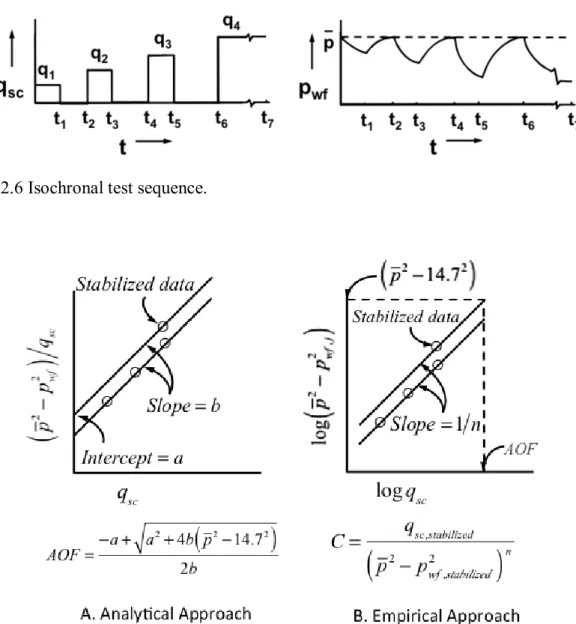
In the basic application of backpressure tests, called flow-after-flow testing, well is

flowed at minimum four different constant rates until pseudosteady state

(boundary-dominated flow) is established in each flow period (Figure 2.4). Using the stabilized

bottomhole pressures at the end of each flow period, a plot of





(Figure 2.5 A) or log





through the data in Figure 2.5 A, the constants, a and b, of Eq. 2.37 and the absolute open

flow potential (AOF) are obtained. Similarly, from the straight line fitted through the data in

31 Figure 2.4 Flow-after-flow test sequence.

Figure 2.5 Flow-after-flow test analysis: A. Analytical approach using Eq. 2.37 and B. Empirical approach of Rawlins and Schellhardt (1936) using Eq. 2.41.

The practical limitation of flow-after-flow tests is the long production periods,

especially in tight formations, to reach stabilized flow during each constant-rate period.

Isochronal testing is an approach to alleviate this problem by using transient flow data. The

basis of isochronal testing is the idea that at a given time, there should be an effective

drainage radius, r , of the well and the transient flow equation should be expressed in terms _d

32

The transient inflow performance equation for a vertical gas well in a cylindrical

reservoir is given by 2 2 2 1 1, 422 ln 2 1, 688 g p pg wf g p tp w q z T kt p p s D q kh c r          _ _    _{ }    (2.42)

If we use the definition of effective drainage radius during transient flow given in Eq.

2.30, we can also write Eq. 2.42 as follows:

2 2 1, 422 g p pg ln d 0.75 wf g w q z T r p p s D q kh r        _{  }   _     (2.43) or, equivalently,

 

 

1, 422 ln for transient flow

2 1, 688

ln 0.75 for pseudosteady state

p pg p tp w d w a t z T kt s kh c r r s r                _{ }  _{   }      _{    } _{   }  (2.45) and 1, 422 pz Tpg b D kh   (2.46)

Comparing Eq. 2.44 with Eq. 2.37, we can conclude that for a fixed flowing time t at

different rates, transient data can be used to obtain the slope of the stabilized data. Based on

this observation, a sequence of equal flow periods at different rates interrupted by shut-ins

33

Figure 2.7 is a sketch of the isochronal test analysis by using the analytical and empirical

equations.

Figure 2.6 Isochronal test sequence.

Figure 2.7 Isochronal test analysis: A. Analytical approach using Eq. 2.37 and B. Empirical approach of Rawlins and Schellhardt (1936) using Eq. 2.41.

The key point to note from the discussion of isochronal testing here is that the slope, b,

(or the power index, n) of the stabilized deliverability equation can be obtained from transient

data. However, without having a stabilized data point, the intercept, a, (or the coefficient, C)

cannot be obtained and the stabilized deliverability equation cannot be constructed.

34

included in the coefficient, a. Therefore, unless a stabilized data point exists; that is, at least

one reference point during boundary dominated flow is available, the drainage area of the

well, gas in place, and the recovery factors cannot be obtained from transient production data

analysis. This is key motivation of the work presented in this thesis.

2.5 Trilinear Flow Model for Fractured Horizontal Wells

In this thesis, the analytical trilinear flow model proposed by (Brown et al., 2009) will

be used to simulate the production performances of fractured horizontal wells in shale. The

choice of the model is completely arbitrary and solely based on its simplicity and

convenience. The general idea of the work proposed in the thesis is independent of the model

used to represent the production performances and can be easily extended to any other

analytical or numerical model.

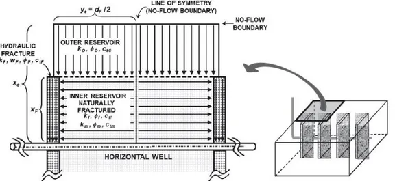
The trilinear flow model considers three flow regions; the outer reservoir beyond the

hydraulic fractures, the inner reservoir (SRV) between hydraulic fractures, and the hydraulic

fracture itself (Figure 2.8). In this model there are three linear flows; from outer reservoir to

inner reservoir, from inner reservoir to hydraulic fractures, and from hydraulic fractures to

wellbore. By using the continuity of flux and the equality of pressures at the boundaries, the

linear flows in these three regions are coupled.

The trilinear flow model is generated to apply to a multiply fractured horizontal well

in a low matrix permeability reservoir (Brown et al., 2009). There are some simplifying

assumptions related to fluid flow and geometry of the system. The most important

assumption is the dominance of linear flow regimes. This model assumes linear flows in all

three flow-regions, which are combined at the associated boundaries of the regions by the

continuity of flux and pressure. Different properties are possible for each flow region. The

35

equally spaced and have identical properties. However, hydraulic fractures have finite

conductivity. The matrix permeability is very low and there is no significant contribution to

production by the outer reservoir. Flow in the outer reservoir is perpendicular to flow in the

inner reservoir, whereas it is parallel to flow in hydraulic fractures (Brown et al., 2009).

Figure 2.8 Schematic of the trilinear flow model representing three contiguous flow regions for a multiply fractured horizontal well (Brown et al., 2009).

The trilinear flow solution is given in Laplace transform domain by









In this work, Stehfest’s (1970) numerical Laplace inversion algorithm has been used

to invert the results into the time domain. The trilinear flow solution in Eq. 2.47 is given in

terms of dimensionless variables. The definitions of dimensionless variables are given below:

Dimensionless pressure, p : _D





36 I

k : inner reservoir permeability (md)

I

h : formation thickness (ft)

q: hydraulic fracture flow rate (STB/d)

B: formation volume factor (RB/STB)

 : viscosity of oil (cp)

i

p : initial reservoir pressure (psi)

Dimensionless time, t : _D 4 2 2.637 10 I D F t x t x    (2.49)

Here,  is the diffusivity of the inner reservoir (ft_I 2/hr) defined by





x : hydraulic fracture half length (ft)

 : porosity (fraction)

t

c : total compressibility (psi-1)

37 D F x x x  (2.51) and D F y y x  (2.52)

where x _and y are the distances in the x- and y-directions, respectively, (ft).

Dimensionless width of the hydraulic fracture:

F D F w w x  (2.53)

where w is the width of the hydraulic fracture (ft). _F

Dimensionless fracture conductivity:

F F FD I F k w C k x  (2.54)

where k_F is the hydraulic fracture permeability (md).

The parameter defined by _F in Eq. 2.47 incorporates the properties of the three flow regions

and their interactions into the solution. The definition of _F is given by

2 _F F FD FD s C      (2.55) where





38 O O eD RD u y C   _  _   (2.57) and





where  and _F  are the diffusivities of the hydraulic fracture and the outer reservoir, _O

respectively. Also, in Eq. 2.57,

I F RD O e k x C k y  (2.61) where O

k : outer reservoir permeability (md) and y is the distance to reservoir boundary in y-_e

direction (ft).

One of the most important parameters in the trilinear flow model is u involved in Eq.

2.57. This term incorporates the properties of the naturally fractured inner reservoir into the

solution through dual-porosity idealization (Warren and Root 1963 and Kazemi 1969). It is

39

 

usf s (2.62)

where f s is the dual-porosity transfer function between matrix and natural fractures and

 

for a homogeneous inner reservoir f s  . For naturally fractured inner reservoirs, we

 

Swaan-O (1976), and Serra et al. (1983) define the transfer function by

 

 





f s    s s  (2.63)

Storativity and transmissivity ratios used in Eq. 2.63 for transient dual porosity model are

given, respectively, by









The derivation and the other details of the trilinear flow solution are given in Brown et

al. (2009) and will not be repeated here as they are not essential for the general results of this

40 CHAPTER 3

TRANSIENT DRAINAGE AREAS OF FRACTURED HORIZONTAL WELLS

As discussed in Chapter 2, the concepts of radius of influence and transient drainage

area have been well documented in the literature for vertical wells with radial flow geometry.

The same is not valid for linear flow geometry due to hydraulic fractures. In this chapter, we

will derive the radius of investigation of a hydraulic fracture during linear flow and define the

effective drainage area during transient flow. We will extend these definitions to fractured

horizontal wells in tight unconventional reservoirs by using the trilinear flow model (Brown

et al. 2009) and define the concept of contacted reservoir volume (CRV) at the time of

economic depletion. We will verify the transient drainage radius expressions by using the

flow regimes predicted based on the trilinear flow model.

3.1 Transient Drainage Areas of Fractured Horizontal Wells

Here we follow the procedure used by Lee (1982), who derived an expression for the

radius of investigation of a vertical well in a radial flow system, and apply it to fractured

horizontal wells in unconventional reservoirs idealized by the trilinear flow model (Brown et

al. 2009) shown in Figure 3.1. Two sets of results will be derived in this section. For the first

set, we will focus on the inner reservoir (SRV) between hydraulic fractures and determine the

transient drainage area of each hydraulic fracture. In the second set of results, the inner

reservoir will be assumed to have depleted and the contribution of the production from the

outer reservoir will be considered. In this case, the transient drainage area of the fractured

horizontal well system will be of interest. The results will be obtained for a homogenous