Comparison of Regression Kriging and Cokriging Techniques to
Esti-mate Soil Salinity Using Landsat Images
Ahmed Eldeiry1
Research Fellow, Decision Support Group, Department of Civil and Environmental Engineering, Colo-rado State University Fort Collins, CO 80523-1372
Luis A. Garcia
Director Integrated Decision Support Group and Professor, Civil and Environmental Engineering De-partment, Colorado State University, Fort Collins, CO 80523-1372
Abstract. The objectives of this study are: 1) to evaluate the best band combinations to es-timate soil salinity with each crop type; 2) to compare regression kriging and cokriging tech-niques when applied to LANDSAT images to generate accurate soil salinity maps; and to com-pare the performance of different crop types: alfalfa, cantaloupe, corn, and wheat as indicators of soil salinity; and. This study was conducted in an area in the southern part of the Arkansas River Basin in Colorado. Six LANDSAT images acquired during the years: 2000, 2001, 2003, 2004, 2005, and 2006 in conjunction with field data were used to estimate soil salinity in the study area. The optimal subset of band combinations from LANDSAT images that correlates best with the soil salinity data was selected. Regression kriging and cokring were applied to 2,915 soil salinity data points collected in alfalfa, cantaloupe, corn, and wheat fields in conjunc-tion with the selected subset band combinaconjunc-tions from the LANDSAT images. Ordinary Least Squares (OLS) was used to regress the correlated band combinations to generate a soil salinity surface. The residuals of the OLS model were kriged and combined with the soil salinity surface generated using the OLS model to produce the final regression kriging soil salinity surface. The same LANDSAT band combinations used with the regression kriging technique were used as secondary data variables with the cokriging technique, while soil salinity data was used as a primary variable. The results show that the best band combinations for estimating soil salinity with different crops are as follows: alfalfa (red, near infrared, and NDVI); cantaloupe (green, and near infrared); corn (near infrared, thermal, and NDVI); and wheat (blue and thermal). The regression kriging technique performed better than the cokriging technique since it was able to capture most of the small variations in soil salinity. Corn fields performed the best and alfalfa fields performed the least. Wheat comes in the second place and cantaloupe comes in the third place.
1. Introduction
Geostatistics is a branch of statistical theory concerned with problems of spatial se-rial data, interpolation and mapping of distributed data, and related problems. Gener-ally, the methods are those of time series analysis, adapted and extended to spatial data (Ripley 1981). Spatial autocorrelation is problematic for classical statistical tests, such
1
Civil and Environmental Engineering Department Colorado State University
Fort Collins, CO 80523-1372 Tel: (970) 491-7620
as ANOVA and ordinary least squares (OLS) regression which assume independently distributed errors (Haining 1990; Legendre 1993). When there is auto-correlation, the assumption of independence is often invalid, and the effects of covariates that are them-selves auto-correlated tend to be exaggerated (Gumpertz et al. 1997). A spatial pattern in the residuals from OLS models may result from failure to include or adequately measure autocorrelation (Lichstein et al. 2002). Kriging models estimate the values at unsampled locations by a weighted averaging of nearby samples. The correlations among neighboring values are modeled as a function of the geographic distance be-tween the points across the study area, defined by a variogram (Miller et al. 2007). Al-though kriging provides a mechanism for combining global and local information in predictions, the ability of the variogram to describe spatial dependence is directly a function of the quantity and quality of the sample data (Miller et al. 2007). The spatial structure of the residuals from the multiple regression models was analyzed using a geostatistical method, the variogram, which has been widely used to analyze spatial structures in ecology (Phillips 1985; Robertson 1987). The empirical variogram, which is a plot of the values of as a function of h, gives information on the spatial de-pendency of the variable. Exponential, gaussian and spherical models were fit to the sample variograms using a weighted least squares method (Robertson 1987).
Triantafilis et al. (2001) used geostatistical methods such as ordinary kriging, re-gression kriging, three-dimensional kriging, and cokriging. These methods were tested with a raw electromagnetic induction instrument (EM-38) in a soil electrical conductiv-ity survey. They compared their methods, on the basis of precision and bias in soil sa-linity estimates, and found that regression kriging performed the best. Eldeiry and Gar-cia (2008a) compared three statistical models (OLS, spatial autoregressive, and a modi-fied residual kriging model) to estimate soil salinity from remote sensing. Their results show that the spatial pattern in the residuals from the OLS models always involve auto-correlation, and when those residuals are kriged and combined with the OLS surface to produce the modified residual kriging model, it provides the best results. Eldeiry et al. (2008) evaluated the use of a modified residual kriging model to reduce the number of soil salinity samples that need to be collected in alfalfa fields. They found that when us-ing modified residual krigus-ing, the number of collected samples can be reduced signifi-cantly with almost the same results.
Howari (2003) used supervised classification, spectral extraction, and matching techniques to investigate the types and occurrences of salt in the Rio Grande valley in the United States-Mexico border. He established the soil groups using soil physio-chemical properties and image elements (absorption-reflectivity profiles, band combina-tions, grey tones of the investigated images, and textures of soil and vegetation covers as they appear in the images). Csillag et al. (1993) used spectral band selection for characterization of the salinity status in soils. They used a modified stepwise principal component analysis approach to select bands for classification of the salinity status. Eldeiry and Garcia (2008b) made a comparison among different satellite images IKO-NOS, LANDSAT, and ASTER to estimate soil salinity in alfalfa and corn fields. They found that the IKONOS images performed the best for both alfalfa and corn fields in es-timating soil salinity. Their study showed that corn fields performed better than alfalfa fields in estimating soil salinity. Aerial photography, videography, infrared thermome-try and multispectral scanners have also been used to detect, map and monitor salt
af-fected soils (Robbins and Wiegand 1990); sources of multispectral images that have been found useful include LANDSAT, SPOT, and the Indian Remote Sensing (IRS) se-ries of satellites (Dwivedi and Rao 1992). Fernández-Buces et al. (2006) correlated soil salinity characteristics with the spectral response of plant species and bare soils. They calculated a Combined Spectral Response Index for bare soils and vegetation by adjust-ing the normalized difference vegetation index (NDVI). Farifteh et al. (2006) mentioned that most salinity studies have focused on severely saline areas and have given less at-tention to the detection and monitoring of slightly or moderately affected areas. They determined that a major constraint was the nature of the satellite images, which do not allow extracting information from the third dimension of the soil body e.g., where salts concentrate in the subsoil. Therefore, they used a transport model to predict the salt dis-tribution in the subsoil. Then data obtained from optical remote sensing sensors was used in simulation models and combined with geophysical surveys to predict different levels of salinization.
Regression kriging involves various combinations of linear regressions and kriging. The simplest model is based on a normal regression followed by ordinary kriging with the regression residuals (Odeh et al. 1995). Cokriging takes advantage of correlation that may exist between the variable of interest and other more easily measured variables (Odeh et al. 1995). Even though cokriging is the most versatile and rigorous statistical technique for spatial point estimation when both primary and secondary (covariate) at-tributes are available, it has been used widely in soil science (Vauclin et al. 1983; Trangmar et al. 1986; Yates and Warrick, 1987). Many studies (Stein et Al, 1988; Stein and Corsten, 1991; Zhang et al., 1992, 1997; Istok et al., 1993) showed superiority of cokriging to ordinary kriging. Others (Shouse et al., 1990; Martinez, 1996) showed that cokriging was only minimally superior to ordinary kriging when auxiliary variables were not highly correlated to primary variables. This suggests that use of auxiliary vari-ables is important to obtaining successful results from cokriging. In addition, to ensure the validity of the estimates made by kriging and cokriging, the semivariograms and cross-semivariograms of the variables must accurately describe the spatial structures.
In this study, the correlation between soil salinity and satellite imagery is evaluated using six satellite images with four different crops as indicators of soil salinity. Regres-sion kriging and cokriging techniques were used to evaluate the correlation between satellite images and soil salinity. A stepwise regression technique and the optimal model function in S+ statistical software were used to select the best band combinations for each crop. The OLS model was used to regress the correlated bands. The kriged re-siduals were added to the OLS surface to produce the final regression kriging model. The same band combinations that were used with the regression kriging model were used with the cokriging technique as secondary variables, while the soil salinity data was used as the primary variable.
2. Site Description
This research was conducted as part of Colorado State University's Arkansas River Basin Salinity Mapping Project in southern Colorado (Figure 1). Crops in this area in-clude alfalfa, corn, wheat, onions, cantaloupe and other vegetables that are irrigated by a variety of systems including border and basin, furrow, center pivots, and a few drip
systems. Salinity levels in the canal systems along the river increase from 300 ppm total dissolved solids (TDS) near Pueblo to over 4,000 ppm at the Colorado-Kansas border (Gates et al. 2002; Gates et al. 2006). This study focused on alfalfa, cantaloupe, corn, and wheat fields. Soil salinity was measured in these fields using an electromagnetic in-duction instrument (EM-38).
Figure 1. The study area.
Table 1 shows the description of the data used in this study. The total number of soil salinity points is 2,915 distributed among alfalfa, cantaloupe, corn, and wheat fields. The fields used in this study represent different ranges of soil salinity from low, moder-ate, to high. Soil salinity data was measured using an EM-38 electromagnetic probe (Eldeiry and Garcia 2008a).
Table 1: Description of soil salinity data collected.
Crop Years Soil Salinity Points Soil Salinity Range (dS/m) Alfalfa 2004; 2005; 2006 989 1.16 – 32.34 Cantaloupe 2004; 2005; 2006 1,102 1.35 – 14.27 Corn 2000; 2001 519 1.43 – 19.50 Wheat 2003; 2005 305 1.48 – 31.26 3. Methodology
3.1. Satellite Images and Image Processing
Six LANDSAT images acquired during July 11, 2000 (LANDSAT 7); July 8, 2001 (LANDSAT 7); July 22, 2003 (LANDSAT 5); August 9, 2004 (LANDSAT 5); July 27,
2005 (LANDSAT 5); and July 30, 2006 (LANDSAT 5) were used in this study. These images were evaluated to assess soil salinity with different crop types. Spatial distortion of the images was corrected using a geometric correction model in ERDAS Imagine 8.7 (ERDAS, 2006), to guarantee that the points on the image match with the same points on the ground. A dark object correction was used to compensate for the effect of atmos-pheric scattering (Song et al. 2001). The Normalized Difference Vegetation Index (NDVI) was added to the bands of the images. The NDVI uses the contrast between red and infrared reflectance as an indicator of vegetation cover and vigor. The LANDSAT 5 images contained seven bands including three visible bands (30 m), two NIR bands (30 m), one thermal band (120 m), and a Mid IR (30 m). LANDSAT 7 images contain three visible bands (blue, green, and red), one near infrared band (NIR), two shortwave infra-red bands (MIR-1, MIR-2) with 30m resolution, a thermal infrainfra-red band (TIR) with 60m resolution, and a panchromatic (PAN) band with 15 m resolution.
3.2. Correlated band combinations
Stepwise regression was used to automatically select the best combination of bands that was correlated with the observed soil salinity data. The stepwise procedure was used to identify the subset of satellite bands that minimizes the AICC (Akaike 1977; Brockwell and Davis 1991). The optimal model function in the S+ statistical software package was used in addition to the stepwise regression model to select the optimal band combinations. In most cases both techniques selected the same bands, if there is any difference, the combination that has the smallest AICC values was used. When the selected band combination was used with the OLS model, if the p value of any band ex-ceeded 0.05, this band was removed to guarantee that the selected bands have strong cross correlation with the soil salinity data.
3.3. Regression Kriging Technique
Regression kriging involves spatially interpolating the residuals from a non-spatial model (e.g. OLS) using kriging, and adding the results to the prediction obtained from the non-spatial model (Goovaerts, 1997). OLS was used to regress the soil salinity data using the values of the corresponding satellite bands and the NDVI index. The OLS re-siduals were kriged and added to the OLS surface (Eldeiry and Garcia 2008a) to pro-duce the final surface of the regression kriging technique. The regression kriging tech-nique modeling process was accomplished as follows:
The coarse-scale variability in the soil salinity as a function of satellite images was explored by multiple regression analysis using the following equation:
(1)
where is the estimated soil salinity at spatial location, s0, are estimated regression coefficients and are the independent variables at spatial location, s0.
A stepwise procedure was used to identify the best subset of satellite bands to include in the regression models that minimized the AICC (Akaike 1977; Brockwell and Davis 1991). The spatial structure of the residuals from the ordinary least squares (OLS) multi-ple regression models was analyzed using a geostatistical method, the variogram, which
has been widely used to analyze spatial structures in ecology (Phillips 1985, Robertson 1987). The sample variogram, is estimated by the following equation:
(2)
where and are the estimated residuals from the multiple regression mod-els at locations and , a location separated by distance h, N(h) is the total number of pairs of samples separated by distance h. The empirical variogram, which is a plot of the values of as a function of h, gives information on the spatial dependency of the variable. Exponential, gaussian and spherical models were fitted to the sample vari-ograms using a weighted least squares method (Robertson 1987) as shown in Figure 3. The variogram model with the smallest AICC was selected to describe the spatial de-pendencies in the soil salinity data.
If the residuals were spatially correlated, ordinary kriging was used to model the spatial distribution of soil salinity in the fields. At every location where there are no samples, estimates of the true unknown residuals, at spatial location, so, were ob-tained using a weighted linear combination of the available samples at spatial locations,
si:
(3)
where the set of weights, takes into consideration the distances between sample loca-tions and spatial continuity, or clustering between the samples. The best fitting sample variogram model was used to describe the spatial continuity in estimating the kriging weights.
3.4. Cokriging Technique
Cokriging equations for estimating a primary variable from a set of variables are ex-tensions of those for kriging. Cokriging works best where the primary variable of inter-est is less densely sampled than the others. Soil salinity is the primary variable and the other variable(s) represent the pixels of the LANDSAT band combinations. The same band combination that was used with the regression kriging was used as secondary vari-ables with the cokriging technique while soil salinity measurements were used as a pri-mary variable.
The semivariogram and cross-semivariogram functions used in regression kriging and cokriging respectively describe the spatial correlation. The estimator for the semivariogram and cross-semivariogram is:
where γij is the semivariance (when i = j) with respect to the random variable zi, h is the
separation distance, n(h) is the number of pairs of zi(xk) and zj(xk) in a given lagged
dis-tance interval (h + dh). When i ≠ j, γij is the cross-semivariogram which is a function of h (Yates and Warrick, 1987).
The cokriging estimate is a linear combination of both the variable of interest and the secondary variables and is given by:
(5)
subject to one of the following sets of linear constraints:
, (6)
or
(7)
where, wr are the kriging weights associated with the n-nearest neighbors, vtr, are the
cokriging weights associated with the m auxiliary variables, utr that are spatially corre-lated to the variable of interest. One of the appealing features of cokriging is that the auxiliary information does not have to be collected at the same data points as the vari-able of interest.
3.5. Model Evaluation
The evaluation of the models is based on the following:
• The accuracy was measured (Kravchenko and Bullock 1999; Schloeder et al. 2001) by the mean absolute error (MAE), which is a measure of the sum of the ab-solute residuals and the root mean square error (RMSE), which is the square root of the sum of the squared residuals. Small MAE values indicate a model with few er-rors, while small values of RMSE indicate more accurate predictions on a point-by-point basis (Schloeder et al. 2001).
The MAE was calculated as follows:
(8)
The RMSE was calculated as follows:
where n is the number of sample sites in the validation sets, are the observed values, and are the estimated values.
• The effectiveness was evaluated using a goodness-of-prediction statistic (G) (Agterberg 1984; Kravchenko and Bullock 1999; Guisan and Zimmermann 2000; Schloeder et al. 2001). The G-value measures how effective a prediction might be relative to that which could have been derived by using the sample mean (Agterberg 1984):
(10)
where is the observed value of the ith observation, is the estimated value of the ith observation, and is the sample mean. A G-value equal to 1 indicates perfect predic-tion, a positive value indicates a more reliable model than if the sample mean had been used, a negative value indicates a less reliable model than if the sample mean had been used, and a value of zero indicates that the sample mean should be used.
4. Results And Analysis
The best bands combinations were selected based on the criteria that the p value of each band be less than 0.05 while the AICC value of the selected band combination be the smallest. The selected band combinations for each crop were: alfalfa: red, near in-frared, and NDVI; with spectral resolutions of (0.63 - 0.69 um), (0.76 - 0.90 um), and (0.63 - 0.9 um); cantaloupe: blue and green with spectral resolutions of (0.45 - 0.52 um) and (0.51 – 0.60 um); corn: near infrared, thermal, and NDVI with spectral resolu-tions of (0.76 - 0.90 um), (8 - 12 um), and (0.63 - 0.9 um); and wheat: blue and thermal with spectral resolutions of (0.45 - 0.52 um) and (8 - 12 um).
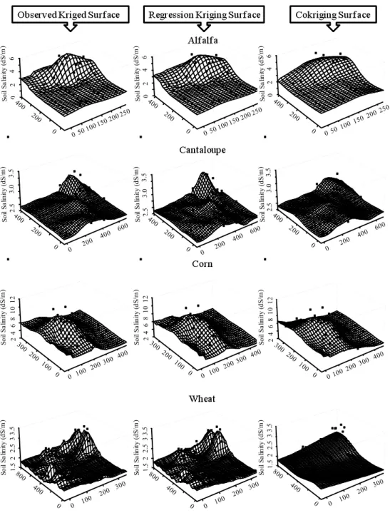
Figure (2) shows a comparison between examples of the generated surfaces using regression kriging and cokriging for the alfalfa, cantaloupe, corn, and wheat fields. The observed kriged surfaces as well as the observed soil salinity points were displayed as a reference for the regression kriging and cokriging models. The regression kriging model performed better than the cokriging model. The regression kriging model was able to capture a lot of variations in the different fields. The cokriging model preformed as a trend surface since it was not able to capture a lot of variations in soil salinity. All the generated surfaces using the regression kriging model are closer to the observed points and the generated surfaces of the observed points than those of the cokriging model.
Figure (3) shows a comparison between regression kriging and cokriging for alfalfa, cantaloupe, corn, and wheat using MAE, RMSE, and G parameters. Most of the values of MAE and RMSE of regression kriging are less than those of cokriging. This makes the accuracy of the regression technique higher than cokriging technique. Also, most of the G values of the regression kriging are closer to 1 than those of cokriging which makes the effectiveness of the regression kriging better than the cokriging technique.
Figure 2. Comparison between examples of the generated surfaces using regression kriging and cokrig-ing from alfalfa, cantaloupe, corn, and wheat fields.
Figure 3. MAE, RMSE, G values of regression kriging and cokriging techniques for alfalfa, cantaloupe, corn, and wheat fields.
5. Conclusion
This study shows that satellite images can be used for better estimation of soil salin-ity. Regression techniques have an advantage over cokriging techniques in that they capture the small variations in estimating soil salinity. The advantages of regression kriging over cokriging may be attributed to the fact that the OLS model regress the cor-related combinations and only a fraction of each combination is used. For cokriging the whole correlated bands are added to the interpolation technique as auxiliary variables. Corn fields provide the estimation for soil salinity while alfalfa fields provide the worst. The low performance of alfalfa may be attributed to the multiple cuts of alfalfa during the growing season which means that the alfalfa biomass can change significantly de-pending on the harvest dates and satellite image acquisition dates. The behavior of al-falfa is different than the other crops (cantaloupe, corn, and wheat) which after planting increase in biomass until full cover. Another fact that might contribute to the poor per-formance of estimating soil salinity in alfalfa fields is the presence of weeds in high sa-linity spots in alfalfa fields which generate a false indication of alfalfa biomass.
6. References
Agterberg, F. P. (1984). “Trend surface analysis.” Spatial statistics and models, Gaile, G. L. and C. J. Willmott, eds., Reidel, Dordrecht, Holland, 147–171.
Akaike, H. (1977). "On entropy maximization principle." Applications of Statistics, P. R. Krish-naiah, ed., North-Holland Publishing Co., Amsterdam, Holland, 27-41.
Brockwell, P. J. and Davis, R. A. (1991). Time series: Theory and methods, Springer, New York, New York.
Csillag, F., Pásztor, L., Biehl, L. L. (1993). “Spectral band selection for the characterization of salinity status of soils.” Remote Sens. Environ., 43(3), 231-242.
Dwivedi, R. S. and Rao, B. R. M., (1992). “The selection of the best possible LANDSAT TM band combination for delineating salt-affected soils.” Inter. J. Remote Sensing, 13(11), 2051–2058.
Eldeiry, A. and Garcia, L. A. (2008a). “Detecting Soil Salinity in Alfalfa Fields Using Spatial Modeling and Remote Sensing." Soil Sci. Soc. Am. J., 72(1), 201-211.
Eldeiry, A. and Garcia, L. A. (2008b). Spatial Modeling of Soil Salinity Using Remote Sensing, GIS, and Field Data, VDM Verlag, Saarbruken, Germany.
Eldeiry, A., Garcia, L. A., and Reich, R. M., (2008). “Soil Salinity Sampling Strategy Using Spatial Modeling Techniques, Remote Sensing, and Field Data." J. Irrig. Drain. Engin., 134(6), 768-777.
ERDAS Imagine, (2006). ERDAS Inc., Leica Geosystems, 2801 Buford Highway, Atlanta, GA 30329.
Farifteh, J., Farshad, A., and George, R. J. (2006). "Assessing salt affected soils using remote sensing, solute modeling, and geophysics." Geoderma, 130, 191-206.
Fernández-Buces, N., Siebe, C., Cram, S., and Palacio, J. L. (2006). “Mapping soil salinity us-ing a combined spectral response index for bare soil and vegetation: A case study in the former lake Texcoco, Mexico.” J. Arid Environ., 65(4), 644-667.
Gates, T. K., Burkhalter, J. P., Labadie, J. W., Valliant, J. C., and Broner, I. (2002). “Monitor-ing and model“Monitor-ing flow and salt transport in a salinity-threatened irrigated valley.” J. Irrig. Drain. Engin., 128(2), 87-99.
Gates, T. K., Garcia, J. C., and Labadie, J. W. (2006). “Toward optimal water management in Colorado’s Lower Arkansas River Valley: Monitoring and modeling to enhance agriculture and environment.” Colorado Water Resources Research Institute, Completion Report No. 205.
Goovaerts, P. (1997). Geostatistics for natural resource evaluation, Oxford University Press, New York, New York.
Guisan, A. and Zimmermann, N. E. (2000). “Predictive habitat distribution models in ecology.” Ecological Modelling, 135(2-3), 147-186.
Gumpertz, M. L., Graham, J. M., and Ristaino, J. B. (1997). “Autologistic model of spatial pat-tern of Phytophthora epidemic in bell pepper: effects of soil variables on disease presence.” J. Agric. Biolog. Environ. Stat., 2(2), 131-156.
Haining, R. (1990). “Spatial data analysis in the social and environmental sciences.” Cambridge University Press, Cambridge, England.
Howari, F. M. (2003). “The use of remote sensing data to extract information from agricultural land with emphasis on soil salinity.” Australian J. Soil Research, 41(7), 1243-1253. Istok, J.D., J.D. Smyth, and A.L. Flint. (1993). “Multivariate geostatistical analysis of
ground-water contaminant: A case history.” Ground Water, 31:63–74.
Kravchenko, A. and Bullock, D. G. (1999). “A comparative study of interpolation methods for mapping soil properties.” Agron. J., 91, 393-400.
Legendre, P. (1993). “Spatial autocorrelation: trouble or new paradigm?” Ecology, 74(6), 1659– 1673.
Lichstein, J. W., Simons, T. R., and Franzreb, K. E. (2002). “Landscape effects on breeding songbird abundance in managed forests.” Ecol. Appl., 12(3), 836–857.
Martinez, C.A. (1996). “Multivariate geostatistical analysis of evapotranspiration and precipita-tion in mountainous terrain.” J. Hydrology. 174,19–35.
Miller, J., Franklin, J., and Aspinall, R. (2007). “ Incorporating spatial dependence in predictive vegetation models.” Ecol. Modelling, 202(3-4), 225-242.
Odeh, I. O. A., McBratney, A. B., and Chittleborough, D. J. (1995). “Further results on predic-tion of soil properties from terrain attributes: Heterotopic cokriging and regression-kriging.” Geoderma, 67(3-4), 215–226.
Ripley, B. D. (1981). Spatial statistics, John Wiley and Sons, New York, New York.
Robertson, G. P. (1987). “Geostatistics in ecology: Interpolating with known variance.” Ecol-ogy, 68(3), 744-748.
Robbins, C. W. and Wiegand, C. L. (1990). “Field and laboratory measurements.” Agric. salin-ity assess. and manage., Tanji, K. K., ed., ASCE, New York, New York, 203-219.
Schloeder, C. A., Zimmermann, N. E., and Jacobs, M. J. (2001). “Comparison of methods for interpolating soil properties using limited data.” Soil Sci. Soc. Am. J., 65, 470–479.
Shouse, P.J., T.J. Gerik, W.B. Russell, and D.K. Cassel. (1990). “Spatial distribution of soil par-ticle size and aggregate stability index in a clay soil.” Soil Sci., 149,351–360.
Song, C., Woodcock, C. E., Seto, K. C., Lenney, M. P., and Macomber, S. A. (2001). “Classifi-cation and change detection using LANDSAT TM data: When and how to correct atmos-pheric effects?” Remote Sens. Environ., 75(2), 230-244.
Stein, A., and L.C.A. Corsten. (1991). “Universal kriging and cokriging as a regression proce-dure.” Biometrics 47,575–588.
Stein, A., W. van Dooremolen, J. Bouma, and A.K. Bregt. (1988). “cokriging point data on moisture deficit.” Soil Sci. Soc. Am. J. 52,1418–1423.
Trangmar, B. B., Yost, R. S., Wade, M. K., Uehara, G., and Sudjadi, M. (1987). “Spatial varia-tion of soil properties and rice yield on recently cleared land.” Soil Sci. Soc. Am. J., 51,668– 674.
Triantafilis, J., Odeh, I. O. A., and McBratney, A. B. (2001). "Five geostatistical models to pre-dict soil salinity from electromagnetic induction data across irrigated cotton." Soil Sci. Soc. Am. J., 65(3), 869-878.
Vauclin, M., Vieira, S. R., Vachaud, G., and Nielsen, D. R. (1983). “The use of cokriging with limited field observations.” Soil Sci. Soc. Am. J., 47, 175-184.
Yates, S. R. and Warrick, A. W. (1987). “Estimating soil water content using cokriging.” Soil Sci. Soc. Am. J., 51, 23-30.
Zhang, R., D.E. Myers, and A.W. Warrick. (1992). “Estimation of the spatial distribution of the soil chemicals using pseudo cross-variograms.” Soil Sci. Soc. Am. J. 56,1444–1452.
Zhang, R., P. Shouse, and S. Yates. (1997). “Use of Pseudo-Crossvariograms and cokriging to improve estimates of soil solute concentrations.” Soil Sci. Soc. Am. J. 61,1342–1347.