Stock Market Anomalies: The Day-Of-The-Week-Effect: An empirical study on the Swedish Stock Market: A GARCH Model Analysis

Stock market anomalies:

The day-of-the-week-effect

An empirical study on the Swedish stock market:

A GARCH model analysis

MASTER THESIS WITHIN: Business Administration NUMBER OF CREDITS: 30 ECTS

PROGRAMME OF STUDY: Civilekonomprogrammet AUTHORS: Alexander Abrahamsson and Simon Creutz JÖNKÖPING May 2018

Acknowledgements

This thesis contributed to the authors’ deeper knowledge within finance and especially within statistics.

The authors are thankful to their tutor Fredrik Hansen for all the incredible support and much appreciated advice during the thesis writing process. A further thanks to all the other supporting teachers at JIBS for their patience and knowledge in responding to our questions.

The authors are grateful to the members of their thesis writing seminar group and are also grateful for the constructive feedback from the opponents at the final opposition seminar.

The authors would like to devote their appreciation to Robert Van Fossen (enrolled at Fordham University, New York, and employed at Citibank. U.S.A) for reviewing this thesis.

Master Thesis in Business Administration

Title:

Stock market anomalies: The day-of-the-week-effect

Authors:

Alexander Abrahamsson and Simon Creutz

Tutor:

Fredrik Hansen

Date:

2018-05-20

Key terms: Market Efficiency, Day-of-the-week effect, Volatility clustering, Leverage

effect, GARCH

Abstract

Background:

The day-of-the-week effect has been a widely studied field ever since the concept was introduced in the early 1970s. Historically, negative returns on Mondays have been the most common finding. In line with improved market efficiency, researchers have started to question the existence of this anomaly.

Purpose:

The purpose of this study is to examine the weak-form efficiency level within the Swedish stock market by using sophisticated statistical approaches. The authors aim to investigate if the day-of-the-week effect was demonstrated between 2000 and 2017.

Method:

To properly provide answers to this investigation, a quantitative

study has been conducted on the OMXS30. The data has been analysed by using different

kind of sophisticated statistical methods such as GARCH and TGARCH.

Conclusion:

The results show that the

day-of-the-week

effect was not

demonstrated within the OMXS30 during this time period, providing evidence for

improved market efficiency.

Table of Contents

1

Introduction ... 6

1.1

Background ... 6

1.2

Problem ... 7

1.3

Purpose ... 7

1.4

Hypothesis ... 7

1.5

Delimitations ... 8

1.6

Abbreviations ... 9

2

Theoretical background ... 10

2.1

Efficient markets ... 10

2.1.1

Samuelson´s dictum ... 11

2.1.2

The random walk hypothesis ... 12

2.2

Market Anomalies ... 12

2.2.1

Leverage effect ... 14

2.2.2

Volatility Clustering ... 14

2.3

Behavioural finance ... 14

3

Literature review ... 16

3.1

Summary of previous findings ... 16

3.2

Review of pre-2000 studies ... 17

3.3

Review of post-2000 studies ... 20

4

Method ... 24

4.1.1

Method Summary ... 24

4.1.2

Scientific Philosophy ... 24

4.1.3

Scientific Approach ... 25

4.1.4

Research Method ... 25

4.1.5

Research Purpose ... 25

4.1.6

Time Horizon ... 26

4.1.7

Data Sample Selection ... 26

4.1.8

Data Collection ... 27

4.2

Statistical Theory ... 27

4.2.1

Computation of Returns ... 27

4.2.2

Volatility ... 27

4.2.3

Comparing mean using T-stat ... 28

4.2.4

Model of the day-of-the-week effect ... 28

4.2.5

Test for heteroscedasticity ... 29

4.2.6

GARCH (1/1) ... 29

4.2.7

TGARCH (1/1) ... 30

4.3

Quality Criteria ... 31

4.3.1

Reliability ... 31

4.3.2

Validity ... 31

4.3.3

Replicability ... 31

4.3.4

Generalisability ... 32

4.3.5

Source Criticism ... 32

5.1

Descriptive Statistics ... 34

5.2

T-test for mean ... 35

5.2.1

Sample 1 ... 35

5.2.2

Sample 2 ... 35

5.2.3

Sample 3 ... 36

5.2.4

Full Period ... 36

5.3

Ordinary least squares regression ... 37

5.3.1

Sample 1 ... 37

5.3.2

Sample 2 ... 38

5.3.3

Sample 3 ... 38

5.3.4

Full Period ... 39

5.4

Test for Heteroscedasticity ... 39

5.5

ARCH/GARCH/TGARCH ... 41

5.5.1

Sample 1 ... 41

5.5.2

Sample 2 ... 41

5.5.3

Sample 3 ... 41

5.5.4

Full Period ... 42

6

Analysis ... 43

6.1

Non-existing day-of-the-week effect ... 43

6.2

Evidence on Leverage Effect ... 45

6.3

Evidence on Volatility Clustering ... 46

7

Discussion ... 48

8

Conclusion ... 52

9

References ... 53

10

Appendix ... 56

List of Tables

Table 1: Different types of stock market anomalies ... 13

Table 2: Findings from additional investigations regarding the day-of-the-week effect ... 16

Table 3: Descriptive statistics for Sample 1. ... 35

Table 4: Descriptive statistics for Sample 2. ... 35

Table 5: Descriptive statistics for Sample 3. ... 36

Table 6: Descriptive statistics for Full Period. ... 36

Table 7: OLS regression for Sample 1. ... 37

Table 8: OLS regression for Sample 2. ... 38

Table 9: OLS regression for Sample 3. ... 38

Table 10: OLS regression for Full Period. ... 39

Table 11: Breusch-Pagan test for heteroscedasticity... 40

Table 12: ARCH/GARCH/TGARCH output for Sample 2. ... 41

Table 13: ARCH/GARCH/TGARCH output for Sample 3. ... 41

Table 14: ARCH/GARCH/TGARCH output for Full Period. ... 42

List of Figures

Figure ii: The value function of prospect theory ... 15

Figure iii: Data sample timeline. ... 27

Figure iv: Histogram graphs fit with normal distribution for all weekdays and the full period .. 34

Introduction

1 Introduction

In this section the authors will give an introduction to their study. First, the background will be presented followed by a problem formulation and purpose. In addition, the hypothesis will also be explained, followed by a list of the delimitations and abbreviations.

1.1

Background

In the 1970, the Efficient Market Hypothesis was established by Eugene Fama. The hypothesis seeks to explain how market efficiency can be described and tested within three categories: the weak-form efficiency, semi-strong efficiency, and strong-form efficiency. However, Fama describes an efficient security market as a market where prices fully reflect all available information. Moreover, Fama argues that prices in an efficient market should follow a random walk and thus making it impossible to predict future security prices using only historical security price data.

Furthermore, evidence from statistical tests contradicts with the efficient market assumptions made by Fama. Seasonal patterns, such as what month or what weekday it is, tend to affect the returns on the stock market. Since the concept of these phenomena is going in the opposite direction of the idea of efficient markets, these are called market anomalies. Therefore, market anomalies have been a well-studied issue in finance, with an emphasis on theday-of-the-week effect beginning in the middle of the 20th _{century. Pioneers in testing stock markets for anomalies}

were researchers as: Frank Cross, Kenneth French, Michael R. Gibbon and Patrick Hess, and Donald B. Keim and Robert F. Stambaugh.

Anomalies can be described as unexpected price behaviour in the market. The day-of-the-week effect is one form of a seasonal anomaly and it is one of the most heavily investigated topics. Early studies, like Cross (1973) and French (1980), have shown that there exists a negative Monday effect, meaning essentially that mean returns on Mondays are negative. The existence of this effect contradicts to the EMH, suggesting that there should be no observable pattern of return in the market. Moreover, this could give investors a possibility to earn positive risk-adjusted returns (RAR). More recent studies, like Steeley (2001) and Kohers et al. (2004) suggests that the stock markets are more efficient today, causing the day-of-the-week effect to slowly disappear.

Introduction

Weighing the evidence for market anomalies against the more recent arguments of Kohers et al. and Steeley; the question remained – do these aforementioned anomalies exist today in our modern, more efficient markets?

1.2

Problem

Using data from 1978-1984, Claesson (1987) found evidence of a day-of-the-week effect onthe Swedish stock market. This is in accordance with the findings of Cross (1973), French (1980), and Gibbon and Hess (1981) regarding the U.S. stock market. Modern studies of market efficiency, like Steeley (2001) and Kohers et al. (2004) suggests that stock markets have become more efficient today. Applying the findings of Steeley and Kohers et al., one might argue that the findings of Claesson on the Swedish stock market are rather outdated. This, therefore, mandates a need for a new investigation explaining the existence of the day-of-the-week effect on the Swedish stock market using more recent data.

This leaves us with the opportunity to adjust a knowledge gap in the research about the stock market efficiency in Sweden. By using recent data, the authors can provide findings regarding a potential day-of-the-week effect in Sweden.

1.3

Purpose

The purpose of this study is to examine the weak-form efficiency level on the Swedish stock market by using sophisticated statistical approaches. Specifically, the authors aim to determine the disappearance of the day-of-the-week effect in Sweden between 2000 and 2017.

1.4

Hypothesis

Testing for daily mean return using t-stat:

H0: 𝛷𝛷𝑡𝑡 = 0

H1: The daily mean return for the weekday is not equal to 0

Where Φdenotes the daily mean return and t represents the weekday. By rejecting the null hypothesis, the authors can conclude that the Swedish stock market is weak-form inefficient.

Introduction

H0: 𝛷𝛷₁= 𝛷𝛷₂ = 𝛷𝛷₃ = 𝛷𝛷₄ = 𝛷𝛷₅

H1: At least one of the weekdays is different from the others

By rejecting the null hypothesis, the authors can conclude that the Swedish index OMXS30 is weak-form inefficient.

Testing for heteroscedasticity using the Breusch-Pagan test:

H0: Constant variance (homoscedasticity)

H1: Non-constant variance (heteroscedasticity)

By rejecting the null hypothesis, the data is heteroscedastic.

Testing for volatility clustering:

H0: 𝛽𝛽 = 0 𝛼𝛼 = 0

H1: 𝛽𝛽 ≠ 0 𝛼𝛼 ≠ 0

A rejection of the null hypothesis suggest that volatility clustering is present in OMXS30.

Testing for Leverage effect:

H0: 𝛾𝛾 = 0

H1: 𝛾𝛾 ≠ 0

A rejection of the null hypothesis suggest that a Leverage Effect is present in OMXS30.

1.5

Delimitations

The aim of this study is to give an indication of the efficiency level of the Swedish stock market through a specific investigation of the day-of-the-week effect. This sets aside the plausible impact of other market anomalies such as the January effect or the turn-of-the-month effect. The limited time frame and resources the authors possessed have compelled us to complete the study by using solely the OMXS30 index, with the motivation that this is still a reasonable approximation of the aggregate Swedish stock market given the authors presumptions.

Introduction

The authors have made the choice to exclusively investigate the weak form inefficiency of the Swedish stock market in order to limit this study. Additionally, tax- and transaction costs will not be taken into account in this study for practical reasons. These standpoints are in line with the arguments of Claesson (1987) regarding studies within the similar field of efficient markets.

1.6

Abbreviations

CRSP - Centre for Research in Security Prices

EGARCH- Exponential Generalised Autoregressive Conditional Heteroscedasticity EMH- Efficient Market Hypothesis

GARCH- Generalised Autoregressive Conditional Heteroscedasticity NPV- Net Present Value

OLS- Ordinary Least Squares

PSBR - The Public Sector Borrowing Requirement RAR- Risk Adjusted Return

Theoretical Background

2 Theoretical background

In the following part, the authors will introduce the relevant theories to the field of the aforementioned problem. The authors begin with broadly explaining the concept of efficient markets followed by the introduction of market anomalies. This is followed by a brief explanation of the topic of behavioural finance.

2.1

Efficient markets

The Nobel laureate Eugene Fama (1970) defines efficient markets as a situation in which firms can make production-investment decisions in which investors can invest in different securities under the assumption that market prices at all-time fully reflects all available information. If all available information is incorporated in the stock prices, an investor should also be able to extract information from the stock prices.

Furthermore, Fama (1970) argues that efficient markets tend to be composed of a large number of rational and profit maximizing agents who actively competes to predict future market values of individual securities. If a market is efficient at any point in time, the actual price of a security is an appropriate estimate of its intrinsic value.

From a theoretical perspective, Fama (1970) claims that the ideal market would entail no transaction costs in trading securities and that all available information could be obtained for the market participants at no cost. Furthermore, all market participants would agree on the implication of current information for current prices and distributions for future prices. This condition is characterised by a completely frictionless market, hence the prices would reflect all available information. However, in practice, these conditions are not possible to satisfy to a full extent. Moreover, the efficient market hypothesis is only concerned with whether stock prices at just any point in time reflect all available information.

Fama (1970) claims that market efficiency can be categorised and tested into three forms: weak form-, semi-strong-, and strong form efficiency. These forms describe the hypothesis in regard to what extent the prices fully reflect all available information in the market. Weak-form efficiency does only include past prices or past returns as available information in the determination of a share price. Semi-strong form reflects all public information including both historical prices and returns, as well as news and reports. Strong-form efficiency includes historical prices and returns, the availability of public news information, and, in addition, implies that insider information is available for all investors.

Theoretical Background

The statement that “prices should reflect all available information” entails that financial transactions at market prices, using available information, can be regarded as zero-NPV activities. However, the purpose of the categorisation of efficient markets into weak-, semi-strong, and strong-form is to see at what level the hypothesis breaks down when conducting the empirical tests of the efficient market hypothesis.

The empirical support of the weak-form of the efficient market hypothesis is supported by historical financial data. The evidence structure tends to explain that technical trading rules are not consistently profitable and that serial correlation in daily stock returns is close to zero.

The semi-strong form of the efficient market hypothesis is primarily tested by investigating whether prices rapidly adjust to publicly available information, for instance announcements of annual or quarterly earnings.

However, the strong-form of the efficient market hypothesis is tested on the assumption that no individual has higher expecting trading profits than others because he or she has exclusive access to some information.

When the stock market is efficient, the investors can trust the market prices to give the most accurate estimate of value for securities and, in addition, that firms receive fair value for their issued securities. However, in efficient markets, fund managers should not be able to pick securities that consistently outperform the market.

2.1.1 Samuelson´s dictum

Another Nobel Prize laureate, Paul Samuelson (1998) presented the dictum that stock markets are “macro inefficient” but “micro efficient”. This means that the efficient market hypothesis works better for individual stocks when compared to the aggregate market. There is substantial evidence supporting Samuelson´s dictum using data from the U.S. stock market since 1926 (Jung & Shiller, 2005). Markets are “micro efficient” because a minority of the investors can detect deviations from efficiency and can thus potentially make money out of it. In so doing, they eliminateany kind of persistent inefficiency as the mispricing is corrected through their speculative trading activity. Markets are “macro inefficient” due to the presence of waves in the time series of aggregate indexes below and above definitions of fundamental values.

Theoretical Background

2.1.2 The random walk hypothesis

According to Fama (1965) the random walk hypothesis suggests that stock prices follow a random movement when markets are efficient, and therefore it should be impossible to predict future stock prices. The random walk model is highly interlinked with the Efficient Market Hypothesis and suggests that it is impossible to beat or predict the market since the information available occurs with a random distribution. According to this hypothesis, it should not be possible to use historical prices to predict future prices. Therefore, the usage of technical analysis is not relevant since it contains chart patterns and indicators of stock price movements.

2.2

Market Anomalies

Market anomalies, described as unexpected price behaviour in the equity market have been an extensively studied field over the past 40 years. Potentially, investors could take advantage of such mispricing in order to earn abnormal returns. Importantly, the transaction costs and time-varying stock market risk premiums need to be taken into account which may offset the potential gains from such a trading strategy. Hence, a market that appears to be inefficient may actually be efficient if one takes the transaction costs and time-varying stock risk premiums into account. In capital markets, including the stock market, anomalies can be described as a deviation from the prediction according to the Efficient Market Hypothesis. This can further be described as diversion in predictable nonzero risk-adjusted returns (RAR) where a stock with zero RAR is fairly priced according to its risk. Hence, a stock with positive RAR leads to an above-average return in relation to its risk (Zacks, 2011).

Primarily, there are three different types of anomalies. These are the price, firm-size, and calendar anomalies. The price anomaly was originally identified by Basu (1977), who found that stocks with low P/E ratios, also referred to as value stocks, had higher risk-adjusted returns when compared to stocks with high P/E ratios, also known as growth stocks.

The firm-size anomaly was first introduced by Keim (1983) and it is defined as the negative correlation between average returns and firm size. This anomaly demonstrates that it is more likely to gain larger returns from investing in small sized firms other than investing in larger sized firms.

Calendar anomalies, or seasonal anomalies, contradict to the EMH in that returns fluctuates depending upon the season of the year or upon the day of the week. Stock market calendar anomalies can further be defined as abnormal returns that cannot be justified by the EMH and that may have been developed due to reasons such as holidays or weekdays.

Theoretical Background

The day-of-the-week effect is an example of a calendar anomaly where the daily mean return differs across the days of the week. According to the Efficient Market Hypothesis, each daily mean return should be equal to each other:

𝑅𝑅𝑀𝑀𝑀𝑀𝑀𝑀𝑀𝑀𝑀𝑀𝑀𝑀= 𝑅𝑅𝑇𝑇𝑇𝑇𝑇𝑇𝑇𝑇𝑀𝑀𝑀𝑀𝑀𝑀 = 𝑅𝑅𝑊𝑊𝑇𝑇𝑀𝑀𝑀𝑀𝑇𝑇𝑇𝑇𝑀𝑀𝑀𝑀𝑀𝑀= 𝑅𝑅𝑇𝑇ℎ𝑇𝑇𝑢𝑢𝑇𝑇𝑀𝑀𝑀𝑀𝑀𝑀= 𝑅𝑅𝐹𝐹𝑢𝑢𝐹𝐹𝑀𝑀𝑀𝑀𝑀𝑀 Where R is the daily mean return.

Researchers have found it difficult to gain more knowledge regardingwhy the seasonal anomalies like the day-of-the-week effect exists. However, Sias and Starks (1995) found some evidence of why this market anomaly appears. They discovered that investors usually trade less during Mondays, which causes returns to be lower on Mondays when compared to other weekdays. Further, Golder and Macy (2011) found that there is a clear pattern of improving mood during the week, which they argue, could be a reason as to why returns are lower on Mondays.

Table 1: Different types of stock market anomalies

Anomaly type: Definition:

1. Calendar anomalies

Day-of-the-week effect The tendency for different weekdays to have unequal mean returns (Cross, 1973; Gibbon and Hess, 1981; Cai, Li and Qi, 2006)

Weekend effect Daily returns on Mondays are in general lower compared to other weekdays (French, 1980)

January effect Higher returns for small cap stocks in the month of January (Rozeff and Kinney, 1976)

2. Price anomalies

Under-reaction

Stocks tend to underreact to good news, which then

is corrected in the following period, leading to a

higher return at that point in time (Barberis,

Shleifer, and Vishny, 1998)

3. Firm size anomalies

Value stocks versus Growth stocks The negative correlation between average returns and firm size. Small market capitalization stocks tend to outperform large market capitalization stocks (Keim, 1983)

Theoretical Background

2.2.1 Leverage effect

The leverage effect is another form of a market anomaly, which refers to the tendency of there being a negative correlation between a financial asset´s return and its changes in volatility. In general, an increase in asset prices leads to a decrease in volatility, and vice versa (Engle & Ng, 1993). The economic interpretation behind this phenomenon could be described as when a firm’s asset price decline, the firm becomes more leveraged. In other words, the relative value of the firm’s debt rises relative to the value of its equity and, as a result, it is reasonable to expect that the firm’s stock price will become riskier and more volatile (Christie, 1982).

2.2.2 Volatility Clustering

Mandelbrot (1963) argues that large changes in volatility are followed by additional large changes in volatility, weather those changes are positive or negative. Likewise, small changes in volatility are followed by additional small changes in volatility. The concept of volatility clustering, as noted by Cont (2007), can be defined as the tendency for stock prices to cluster together, hence, the result will be that the amplitude of these stock prices will be persistent. Cont (2007) further discuss a variety of mechanisms that can explain volatility clustering. One explanation made by Guillaume et al. (1997) is that volatility clustering may depend on heterogeneity in agents' time scale. Long-term investors focus on the behaviour of stock prices from a long-term perspective while short-term investors focus on the short-term behaviour of stock prices. Moreover, Andersen and Bollerslev (1997) suggests that a further explanation of volatility clustering is the aggregation of information flows during short or long periods of time.

2.3

Behavioural finance

To further clarify the issues of explaining the existence of anomalies on the stock market, behavioural finance has been developed. Behaviouralfinance is based on the idea that investors are consistently neoclassical irrational. Modern economic theory has its standpoint in that the representative agent, for example an investor, is rational in two different ways. Primarily, the agent makes decisions that are consistent with the expected utility theory. Secondly, the agent makes unbiased forecasts about the future. (Thaler, 1999).

Efficient Market Hypothesis assumes that investors process all the information rationally all the time. Therefore, biases like overconfidence, conservatism, representative, and biased self-attribution should not have an impact on the decision-making process (Zacks, 2011).

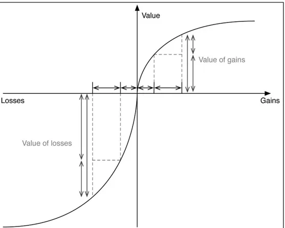
Kahneman and Tversky (1979) initially presented prospect theory in assuming that losses and gains are valued differently. They suggest that individuals may make decisions based on perceived gains instead of perceived losses. In a decision-making situation where, on one hand,

Theoretical Background

one would realize a certain gain and, on the other hand, one would gamble the possibility of a larger gain with the risk of getting nothing, most would choose the former over the latter. This is true even though the uncertain alternative offers a better outcome. To support this, Rao et al. (2011) conducted an experiment of multiple choices in gambling. The result was that both adults and adolescents are similarly loss averse regarding mixed gambles. According to Shefrin and Statman (1984), this can further be applied to trading behaviour on the stock market in a phenomenon known as the disposition effect. This effect demonstrates that investors have a tendency to sell winners too early and hold on to losers for too long.

The diagram below shows that the value of gains is less than the value of losses, although the gain and loss is of equal size.

Figure i: The value function of prospect theory

Literature Review

3 Literature review

In this chapter, the authors will present a research overview of the day-of-the-week effect. This is followed by a systematic review of articles published before and after year 2000.

3.1

Summary of previous findings

The table below broadly summarises some main findings from previous investigations.

Table 2: Findings from additional investigations regarding the day-of-the-week effect

Authors: Data: Findings: Solnik and Bousquet (1990) France

1978-1987

Higher returns on Fridays Negative returns on Tuesdays Dubois and Louvet (1996) USA, Canada,

Hong Kong, Germany, France, UK, Switzerland, Japan, Australia 1969-1992

Negative return on Mondays Positive returns on Wednesdays

Japan and Australia show significantly negative returns on Tuesdays

Oguzsoy and Güven (2003) Turkey

1988-1999

Lower returns on Tuesdays Higher variance on Mondays

Higher returns on Wednesday and Fridays Stavárek and Heryán

(2008) Czech Republic, Hungary, Poland 2006-2012

No clear evidence on the day-of-the-week effect

Literature Review

3.2

Review of pre-2000 studies

Cross (1973) examined the distribution and the relationship of price changes on Fridays and on Mondays. The data that Cross (1973) used included daily closing prices of the Standard and Poor’s Composite Stock Index between the years 1953 to 1970. This data, however, includes in total 844 Mondays and 844 Fridays. Cross (1973) was looking into whether the daily closing prices of the S&P Composite Stock Index advanced or declined on Fridays and Mondays respectively in the data set. Cross found out that this resulted in that the index advanced in 62 percent of all the Fridays and in 39,5 percent of all Mondays. The mean percentage change was also higher on Fridays compared to Mondays. Furthermore, Cross (1973) also researched how the Mondays’ price changes were contingent on Fridays’ price changes. Hence the results showed that in 48,8 percent of the cases where there was an advance on a Friday, the advance on a Friday led to an advance on the following Monday. In the other 313 cases where there was a negative Friday, the subsequent Monday rose in 24 percent of the cases. Furthermore, Cross (1973) found significance of negative Monday returns throughout the whole dataset.

French (1980) used data from the Standard and Poor’s 500 Stock Index during the years 1953 to 1977, which is divided into five five-year periods. Each period shows a negative mean return on Mondays, while all of the other weekday returns are positively distributed. French (1980) found that the lower returns on Mondays are due to some weekend effect, not certainly by a general closed-market effect. French (1980) proposed a trading strategy from based upon the negative Monday returns, as shown by the statistical results. The strategy proposed to buy the S&P portfolio every Monday afternoon and to sell this portfolio on the following Friday afternoon in order to hold cash over the weekend. Ruling out transaction costs, this strategy would have yielded 134 percent in annual average return from 1953 to 1977. In comparison to this, a buy-and-hold strategy would have yielded an annual average return of 55 percent. French (1980) arrives at the conclusion that the persistence of the negative returns on Mondays is the result of market inefficiency.

Gibbon and Hess (1981) examines the day-of-the-week effect regarding asset returns including stocks from the Standard and Poor’s 500 stock index, the Dow Jones 30 stock index and two portfolios of different securities created by the CRSP. One of the portfolios was value-weighted including different securities and one portfolio was an equally-weighted including different securities. These are tested statistically on the equality of the means for each day-of-the-week. The time range of data used in the study was from 1962 to 1978. The study showed that negative

Literature Review

across different security types, such as American treasury bills which shows a below average returns on Mondays. Finally, Gibbon and Hess (1981) argues that the aggregation of returns in portfolios can eliminate the day-of-the-week effect regarding market adjusted returns.

Keim and Stambaugh (1984) takes a further look at this issue by extending the investigation period to 55 years (1928-1982) and by using different portfolios of stocks from the USA. The authors confirm the results of the earlier studies adopted and re-tested in the study. However, Keim and Stambaugh makes an attempt to further explain the measurement error hypothesis that Gibbon and Hess (1981) have brought up in their study. Keim and Stambaugh emphasises that the significantly negative Monday returns and the significantly positive Friday returns are present during these years, regarding the stock indices, and for individual stocks.

Since Cross, French, Gibbon and Hess, and Keim and Stambaugh found out that Monday returns tend to be abnormally low and Friday returns abnormally high, Jaffe and Westerfield (1985) sought for a further explanation of this in the concept of the day-of-the-week effect. Jaffe and Westerfield continues by concluding that the weekend effect exists in the major indices of Japan, Canada, the UK and Australia. Shifting the focus towards explaining the weekend effect, Jaffe and Westerfield start out by investigating the settlement procedures regarding stock purchases in each of the respective countries included in the study. Henceforth, the authors conclude that the settlement effect has no effects on the returns for different weekdays. The settlement procedures in each country should follow a pattern of expected returns on certain days. Since the output of the descriptive statistics shows that the actual returns do not follow this expected pattern, the hypothesis of the settlement impact can be rejected at this point. In conclusion, Jaffe and Westerfield (1985) finds, contradictory to the results of previous studies (Cross, French, Gibbon and Hess, and Keim and Stambaugh), that the lowest mean return occurs on Tuesdays for the Japanese stock market and the Australian stock market. Jaffe and Westerfield (1985) conclude that the integration of foreign currency markets does not offset the weekend seasonality in the foreign stock markets.

Claesson (1987) also takes a point at the day-of-the-week effect using data from OMXS30 in Claesson’s doctoral thesis. This can be regarded as the pioneer work of the day-of-the-week effect in Sweden. Claesson starts out by reviewing earlier important studies of the-day-of-the-week anomaly, included French (1980), Keim and Stambaugh (1984), Lakonishok and Levi (1982), and Jaffe and Westerfield (1985). Claesson agrees with these researchers on the conclusion that Monday returns are most often negative, while the returns toward the end of the week tend to be more positive. Claesson further examines the day-of-the-week effect in Sweden by using stock

Literature Review

return data between the years 1978-1984 for individual stocks listed on the Stockholm Stock Exchange. Mainly, descriptive statistics including mean and standard deviation are presented. Claesson concludes that settlement effects can be a reasonable explanation of the day-of-the-week effect in this return data. Specifically, it is explained by the payment system of stock purchases. Claesson also investigates if there is a correlation between the distributions of the returns in two consecutive years. Claesson further concludes that a day-of-the-week effect it does exist on the Stockholm Stock exchange in the years 1978-1984. However, Claesson argues that this effect tends to be rather small and it implies low practical use for an investor due to transaction costs.

Lee et al. (1990) conducted a study of the day-of-the-week effect with a major focus on the Asian “second tier” stock markets between the years 1980-1988. However, Lee et al. argue that the explanations of the results from earlier mentioned studies, namely that stock returns are significantly different from each other on Mondays and on Fridays and as well as different from the other weekdays in terms of mean returns, can be questioned. Since the explanations of these abnormal patterns are mainly targeting on settlement practices and dividend payment practices, Lee et al. consider these theories of explanation to be rather weak.

Lee et al. (1990) found that the day-of-the-week effect is present in the majority of the Asian stock markets during 1980-1988. Following up on previous studies, their findings are rather consistent with those of Cross, French, and Gibbon and Hess. Hong Kong, Japan, Korea and Singapore show a tendency of a negative mean return on Mondays, but especially on Tuesdays. However, the S&P 500 show greater results of negative Mondays compared to the Asian stock markets under these years. However, the equally weighted US index show mostly negative Monday returns.

An interesting point that Lee et al. make is that dividend payments connected to a day-of-the-week only can be regarded as a partial explanation of the anomalies in returns for certain weekdays. Furthermore, the authors found out that the standard deviation tend to be higher on Mondays and lower on Fridays throughout the data sample period.

Wang, Li, and Erickson (1997) investigate whether the well-known Monday effect exist depending on the week of the month. The sample consists of data from the U.S. stock market for the period 1962-1993. These researchers concluded a negative Monday effect. However, it is most observable in the fourth and fifth week of the month. On the other hand, for the first three weeks the negative Monday effect is not significant. Furthermore, the authors argue that it may be

Literature Review

small differences and the ticker size. However, these findings could help an investor with the transaction timing when the investor decided to trade. The investor could then realize a higher profit from selling before the end of the third week or could also take advantage of abnormally low prices through buying after the fourth Monday of a month.

3.3

Review of post-2000 studies

Steeley (2001) uses daily return data from the FTSE 100 index and announcement data on macroeconomic information variables in the period 1991-1998. The data includes 1803 observations excluding holidays. Steeley investigates the relationships between intraweek news arrival patterns and intraweek return patterns. Steeley chose to use four types of macroeconomic news announcement types as variables to include and test. The author argues that these effects are those that tend to attract the most public information. The variables are: RPI (Inflation, base rate). Unemployment and labour market statistics (wage growth, government borrowing including PSBR), and Broad money supply (M4).

The announcement day’s data also includes announcements of short-term interest rates. The total number of observations of announcement days is 374. From the results table, Steeley concludes that there is a strong tendency for announcement of macro-news to cluster around the center of the week (Tuesdays, Wednesdays and Thursdays). Steeley considers this to be a relevant explanation for intraweek anomalies.

The return-data is sorted for each weekday and a mean of the log returns is calculated. As the results show, there is no evidence of a day-of-the-week effect in the FTSE100. This implies that the means of each weekdays are not statistically different from each other.

Steeley argues that the evolvement of the settlement system is largely contributing to the disappearing day-of-the-week effect. It might be interesting to further investigate how market fluctuation and direction periods can affect weekday patterns. Steeley provides evidence that intraweek news information seasonality can explain the intraweek return seasonality in the FTSE100.

Kohers et al. (2004) investigates whether the mean returns for each trading day are equal to one another on the MSCI World Index. Kohers et al. wanted to test if there have been any improvements in market efficiency and, furthermore, if any demonstrable improvements have caused the of-the-week effect to disappear. The findings from this research show that the

day-Literature Review

of-the-week effect evidently appeared throughout the 1980s, sharply decreased in the 1990´s, and have since faded out almost completely. The authors state that the improvement of market efficiency was the underlying force that caused the day-of-the-week effect to slowly fade out.

Cai, Li, and Qi (2006) examines A- and B- share indices of the Shanghai or Shenzhen stock exchanges by testing the day-of-the-week effect for each week of the month. They found that Monday returns from A-shares indices are significantly negative during the latter half of each month. Further, they found that Tuesday returns for both A- and B-share indexes are negative during the second week of the month. Additionally, they investigated the daily returns without considering which week of the month it is and subsequently found negative returns for Tuesdays. In line with statistical credibility, Cai, Li, and Qi (2006) also controlled for autocorrelation and spillover impacts from regional and international markets. Even with these controls, the results still remained significant.

Guidi (2010) carries out an investigation on the Italian MIB index at a sub-sectoral level. Guidi discovers abnormal returns for financial holdings and financial services on Thursdays as well as Tuesdays. Food, paper and textile, clothing, and industrial miscellaneous also appears to have abnormal returns on Thursdays. Further, Guidi presented evidence that approximately all the sub-sectoral returns did not follow a random walk process according to the efficient market hypothesis.

Golder and Macy (2011) documented a pattern of improving mood during the week. They identified individual seasonal mood rhythms by using data from millions of public tweets. The patterns showed that the aggregate mood tends to increase during the week with people feeling relatively happier at the end of the week as compared to the beginning of the weeks. This is something Zilca (2017) argues to be one of the most important reasons why the day-of-the-week effect exists.

Derbali and Hallara (2016) examine the effect of the day-of-the-week for the Tunisian stock exchange index (TUNINDEX). The authors used daily returns over the period 31 December 1997 to 7 April 2014. In order to extract useful conclusions out of the data, autoregressive heteroscedasticity models, such as GARCH, EGARCH, and TGARCH, were used. The empirical findings are supportive of market inefficiency with a presence of the day-of-the-week effect upon TUNINDEX returns. Specifically, the authors presented evidence on a positive Thursday effect and a negative Tuesday effect. It could be concluded that volatility is persistent, or, in other terms,

Literature Review

established that a positive and highly significant return on Thursdays is present at a 99% confidence level. Furthermore, Wednesday have a positive impact on the TUNINDEX return and Tuesday have a negative impact at a 95% confidence level. The results from the mean equation from the EGARCH and TGARCH confirm the previous findings from the GARCH. This suggests that the TUNINDEX is weak form inefficient. From the variance equation of the GARCH, all the parameters were significant at a 99% confidence level for the three models, which suggests the persistence of volatility within the Tunisian stock market index. The highly significant gamma parameter from the EGARCH and TGARCH show evidence that a leverage effect exists. Derbali and Hallara argue that this means that bad news tends to increase volatility more than good news.

Zilca (2017) studied the day-of-the-week effect in three 18-year sub periods on all stocks listed on NYSE, AMEX, and NASDAQ exchanges. The purpose was to examine the evolution of the day-of-the-week effect over time. The full period runs from 1956-2006, where each sub period is 18 years. By using different types of portfolios, equally weighted (EW), value-weighted (VW), and 10 deciles sorted by market capitalization for smallest and largest capitalization, Zilca tried to find changes in the pattern of the day-of-the-week effect over time. Zilca found that returns increase as the week progresses in the smallest capitalization deciles when taking into account the full period. Furthermore, it was suggested that the reason behind increasing returns during a week is due to a behavioural factor, that mood often tends to increase throughout the week. Zilca also found that the day-of-the-week effect has declined over the years as it is not as clearly evident in the latter years compared to the beginning years of the investigated period. In some of the portfolios, for example the VW portfolio, the effect was totally vanished in the last 18-year sub period.

Gbeda and Peprah (2017) conducted a study of the day-of-the-week effect on the stock markets in Ghana and Kenya by examining daily closing prices and daily returns between the years 2005-2014 on GSE-CI (Ghana) and NSE-20 (Nairobi). Gbeda and Peprah conducted an OLS regression with daily returns as the dependent variable and with four dummy variables representing all weekdays (except for the Monday, which is the intercept in the model) as explanatory variables. The OLS regression does also include an autoregressive term. A rejection of the null hypothesis implies that the stock returns exhibit a day-of the-week-effect.

Furthermore, Gbeda and Peprah also examined the volatility in the two stock markets mentioned above. To do this, a GARCH (1, 1), an EGARCH (1, 1) and a TGARCH (1, 1) - model was used to be able to predict future returns and determine whether the volatility show persistency over

Literature Review

time. Also, the TGARCH was adopted in order to capture the asymmetry effect arising from the tendency of a more pronounced impact from bad news than from good news.

The results from the descriptive statistics show no evidence of a day-of-the-week-effect in Ghana but do show a positive Friday effect in Nairobi. This implies that future stock prices can be predicted in Nairobi but not in Ghana. However, the GARCH show evidence of persistent volatility in Nairobi, implying both α and β are close to one and significant at a 99 % confidence level. However, the TGARCH show that the γ (leverage term) is positive, but not statistically

significant. Hence, it compels Gbeda and Peprah not to reject the null hypothesis (which states that there is no asymmetry effect on the conditional volatility) and to conclude that good and bad news have the same impact on volatility. There was no evidence of conditional volatility in Ghana.

Method

4 Method

In the following chapter, the authors present the mode of procedure. The first part consists of an explanation of the choices and strategies followed by a comprehensive presentation of the statistical methodology. The authors finish this section by assessing and reflecting upon the quality of this study.

4.1.1 Method Summary

This study takes on a positivist philosophy, further taking a deductive research approach. Since the data collection and data analysis method is numerical, the authors have taken a quantitative approach. The study is of explanatory nature, also being cross-sectional regarding the time horizon. However, the authors used non-probability sampling, and further purposive sampling to select what years and stock market data to include in the data sample. The authors selected the OMXS30 Stock Market Index in their study, during an 18-year period between 1999-12-31 and 2017-12-31. This period was divided into three sub-samples of three 6-year periods.

To examine the day-of-the-week-effect, several statistical tests were conducted. Descriptive statistics, an OLS regression with dummy variables, a Breusch-Pagan-test for heteroscedasticity, a GARCH (1, 1) and a TGARCH (1, 1) were all used by the authors.

The quality criteria used to assess the quality of the study were reliability, validity, replicability and generalizability. At the end of the method part, some concluding remarks about research ethics are mentioned.

4.1.2 Scientific Philosophy

The scientific philosophy contains assumptions about the way in which a researcher view the world. Saunders, Thornhill and Lewis (2012) argue that there are several scientific philosophies within research such as: positivism, pragmatism, interpretivism, and realism. This study was conducted using primarily the positivism philosophy.

When using positivism, one takes the position of "the natural scientist", which means that only phenomena that can be observed will lead to an outcome of reliable data. Moreover, the researcher will only take an interest in facts rather than impressions and feelings (Saunders, et al., 2012). Since the authors wish to find out answers regarding the day-of-the-week effect by using quantitative data and applying proven theories the positivistic philosophy was used, as typically made in finance.

Method

4.1.3 Scientific Approach

There are two main research approaches available. These are deduction, which is commonly associated with positivism, and induction, which is commonly attached to interpretivism. Using a deductive approach, the researcher develops a hypothesis or a theory to further design the study to test it. On the other hand, using an inductive approach, the researchers begin by collecting data to develop a theory from it (Saunders, et al., 2012). The authors of this study chose to take a deductive research approach. Since the authors of this study will develop several hypotheses of market efficiency and the day-of-the-week effect to test on financial data, deduction will be the most appropriate research approach.

4.1.4 Research Method

There are two procedures of data collection and analysis, which are either qualitative or quantitative. The selection of this approach is necessary in order to make it possible to analyse the collected data. Quantitative data is mainly based on meanings derived from numbers and returns results in numerical and standardised data. Analysis of this type is primarily conducted by using diagrams or statistics. Qualitative data is based on meanings expressed as words and the analysis is often conducted by using conceptualisation. Since historical stock prices are used in this study and multiple statistical analysis such as GARCH and TGARCH are conducted, the authors conclude that the quantitative approach is the most suitable (Saunders, et al., 2012).

Before the quantitative data has been processed and analysed, in other words, when the data is stated in raw form, it bears no meaningful information. Therefore, the data needs to be processed and analysed in order to convert it into more useful information. After this has been accomplished, it is helpful to convey the data into the forms of charts, graphs, and other visual statistics, which allow the authors to present, describe, explore, and examine trends and relationships within the selected data (Saunders, et al., 2012). Furthermore, the quantitative approach is used to test objective theories by examining different kinds of relationships among some specific variables. This means that it is important to neutralise any subjective influence and to collect information in an objective manner (Creswell, 2014).

4.1.5 Research Purpose

The research purpose can be either exploratory, descriptive, or explanatory. Since this study aims at discovering the relationship between different variables, the explanatory research purpose is the most appropriate of the three. Explanatory research studies aim to explain relationships between variables, often through statistical tests such as correlation in order to clarify relationships (Saunders, et al., 2012).

Method

4.1.6 Time Horizon

There were two approaches to choose from when it came to the planning of this study. The first one is cross-sectional and can be described as a snapshot taken at a particular point in time. On the other hand, there is the other approach that is known as longitudinal. This can roughly be described as the "diary" perspective. The choice of time horizon is closely linked to the research question (Saunders, et al., 2012). Since this study intends to investigate a phenomenon at a point in time, the authors have chosen the cross-sectional approach.

4.1.7 Data Sample Selection

According to Saunders et al. (2012) there are multiple choices of sampling strategies available. These can be divided into two major types, probability sampling and non-probability sampling. Probability sampling is the situation in which the probability of choosing each member of a sample is known and non-zero in its nature. Opposed to this, non-probability sampling means that sample group members are selected non-randomly. This implies there it is zero-chance for some of the population members to be selected. The authors of this study have chosen to use non-probability sampling.

However, there are multiple types of non-random sampling such as purposive sampling, Quota sampling, and snowball sampling. The authors of this study used purposive sampling to select the case to include in the study, namely the OMXS30 stock index. The reason why purposive sampling was chosen is because Claesson (1987) used this sample when testing the day-of-the-week-effect in the 1980s and, furthermore, it is the most appropriate choice in order to enable the authors to answer the research question in the best possible manner taking the Swedish perspective.

Since Claesson (1987) conducted a similar type of study of the day-of-the-week-effect with sample data from the OMXS30, it is natural for the authors to use OMXS30 Index as the selected sample in order to replicate and compare the results from Claesson´s study. However, the time period of the data in Claesson´s study is between 1978 and 1984, a data sample period of 6 years. The authors therefore chose to use three sample periods, each of six years. The first sample period was from 1999-12-31 to 2005-12-31, the second sample period was from 2005-12-31 to 2011-12-31 and, finally, the third sample period was from 2011-2011-12-31 to 2017-2011-12-31. In aggregate, a full sample period of 18 years (from 1999-12-31 to 2017-12-31) was studied. The full sample selection consists of closing prices from 4695 trading days, based on which the return data are calculated. Furthermore, the findings of Kohers et al. (2004) and Steeley (2001) suggest that the day-of-the-week-effect began to fade out from year 2000 and onwards. Pursuant to these findings, it is interesting to divide the full sample set of 17 years to be able to verify if this identified trend is present in the OMXS30 over the time period studied.

Method

The OMXS30 index is a market-weighted index and contains the top 30 companies having the highest turnover on the Swedish stock market. However, it should be noted that the index is revised two times per year. Therefore, the authors have provided the composition of the index from 2018-01-25 in the interest of data consistency.

Figure ii: Data sample timeline.

Source: Own creation

4.1.8 Data Collection

The secondary data retrieved for this study was collected from Thompson Reuters Datastream 2018-01-25. The access to Thompson Reuters Datastream was granted by Jönköping University.

4.2

Statistical Theory

4.2.1 Computation of Returns

After collecting the daily closing prices, the data wasprocessedin order to make it comparable. By computing daily returns it is possible to analyse and to compare the data. The formula used to calculate daily returns is given by equation 1 as stated by Brooks (2008):

𝑅𝑅_𝑡𝑡 = 𝑙𝑙𝑙𝑙( Pt

Pt−1) (1)

where Rt is the contiguously compounded return of the OMXS30, ln is the natural logarithm, Pt

and Pt-1 are the daily closing prices for time t and time t-1 respectively, and t indicates the time,

in this case the day (Brooks, 2008).

4.2.2 Volatility

Volatility can certainly be stated as one of the most important concepts in finance. Volatility is measured as the standard deviation or variance of return, and volatility is often used as a measure

Full Period

Sample 1

Sample 2

Sample 3

Method

of the total risk of a financial asset. Historical estimates of standard deviation are often used to calculate current and future volatility (Brooks, 2008).

Furthermore, the phenomenon of volatility clustering has rendered much research activity. Given the existence of this anomaly, the development of stochastic models in finance has emerged. The most widely used model to capture this phenomenon is GARCH models according to Teyssière and Kirman (2011).

4.2.3 Comparing mean using T-stat

In order to test whether some of the individual weekdays have a daily mean return statistically different from zero, a simple T-stat is conducted by comparing the daily mean return if that return is anything but zero.

4.2.4 Model of the day-of-the-week effect

In order to test for the day-of-the-week effect, statistical regressions analyses have been conducted with the daily index return as the dependent variable and four daily dummy variables as independent variables, and an intercept that reflects Mondays. Each dummy variable takes on a value of one on the particular day, for example the dummy variable for Tuesdaywill be one if it represents a Tuesday and zero otherwise. The intercept consists of the average returns for the first trading day-of-the-week, in this case it is the average return on Mondays. The other dummy variables represent the average deviation of return from the average return on Mondays. Additionally, the one day-lag of index return will be included in the regression which is the autoregressive (AR) term as well as the daily return for the German DAX30. The model for the day-of-the-week effect is stated in equation 2:

𝑅𝑅_𝑡𝑡 = Φ₁+ Φ₂𝐷𝐷_2𝑡𝑡+ Φ₃𝐷𝐷_3𝑡𝑡+ Φ₄𝐷𝐷_4𝑡𝑡+ Φ₅𝐷𝐷_5𝑡𝑡+ ΦR_𝑡𝑡−1+ 𝑅𝑅_{𝐷𝐷𝐷𝐷𝐷𝐷}+ 𝜀𝜀_𝑡𝑡 (2)

where Rt is daily index return on OMXS30, Φ1 is the intercept or the Monday return. Dit are the

daily dummy variables, where D2t is the dummy variable for Tuesday. Φ2 toΦ5 are the coefficients

of the dummy variables. ΦRt-1 is the one day lagged return of the index or the autoregressive (AR)

term. RDAX is the index returns from the German DAX, acting as a control variable in order to

improve the goodness of fit for the model. The error term is denoted as εt is which is normally

distributed.

Then the null hypothesis was tested to see if daily average returns across the weekdays are relatively equal, which would indicate that there is no day-of-the-week effect. This was tested against the alternative hypothesis that average daily returns for the weekdays are not equal, in

Method

other words that at least one day is significantly different from the other days. P-values have been used to determine whether it is significant or not. The null hypothesis that was tested is stated as:

H0: 𝛷𝛷₁= 𝛷𝛷₂ = 𝛷𝛷₃ = 𝛷𝛷₄ = 𝛷𝛷₅

A P-value smaller than 0,05 for any of the weekdays implies that at least one weekday has a significant impact on the index return, which in turn suggests that the day-of-the-week effect exists.

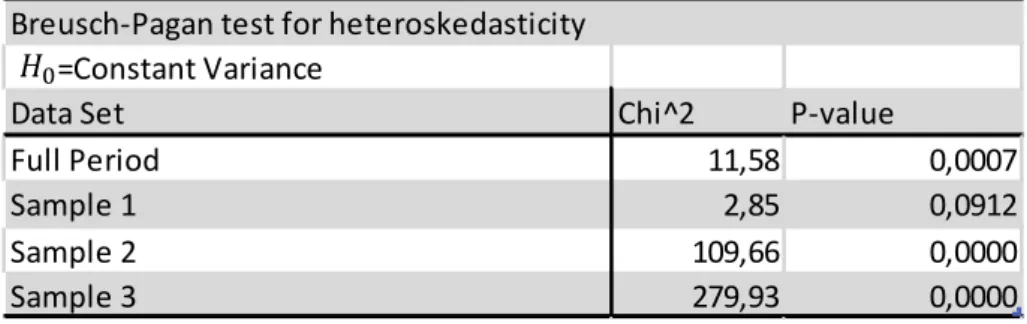
4.2.5 Test for heteroscedasticity

When using the Ordinary Least Squares (OLS) regression model, it is usually assumed that coefficients are fixed, and the disturbances are homoscedastic, which indicates that the variance is constant over time. Breusch and Pagan (1979) argue that this should be questioned. When the requirements regarding homoscedasticity are not met, the efficiency in using a general linear model is weak and it may lead to substantial errors in the estimates. Adjusting for heteroscedasticity by introducing random coefficient variation allows for the potential for the dependent variable to take on different variances at each observation.

The heteroscedasticity can be tested by computing a Breusch-Pagan test where the null hypothesis states that homoscedasticity exists, while the alternative hypothesis indicates the existence of heteroscedasticity. Hence, rejecting the null hypothesis suggests heteroscedasticity, in other words, that there are non-constant volatility in the selected sample. When heteroscedasticity is present, linear regression is not the appropriate statistical model to use, hence a conditional heteroscedasticity test might be appropriate (Breusch & Pagan, 1979).

4.2.6 GARCH (1/1)

Generalised Autoregressive Conditional Heteroscedasticity or the GARCH model was first introduced by Bollerslev (1986) and it was developed to examine volatility in returns. The main difference between GARCH and a simple linear regression is that the GARCH model allows for the variances of errors to be time dependent. The output of a GARCH model estimates the predictability of future stock returns and determines the nature of volatility, in other words if volatility is persistent or not.

A GARCH model consists of two components; a mean equation and a variance equation. The mean equation is stated in equation (2) and the variance equation is specified in equation 3:

Method

where Ht is the conditional variance, ω is the constant term. βht-1 is the GARCH term which

represents theinfluence of new shocks to volatility. The ARCH term is denoted as αε2

t-1, which

measures how intensely the volatility reacts to market shocks. Furthermore, α and β represents the market volatility and these are the variables to be estimated. A large error coefficient α implies that volatility reacts strongly to movements in the market. A large value of the β coefficient means that shocks to conditional variance take long time to fade out, in other words this measures the persistence of volatility (Bollerslev, 1986).

Significant values of α and β imply that historical stock market volatility affects current volatility and that volatility is highly persistent which in turn implies market inefficiency. The main drawback of the GARCH model is that it does not capture the asymmetry effect (leverage effect). The GARCH model tests two different hypotheses, one for the mean equation and one for the variance equation. The hypothesis for the mean equation is the same as that one of the OLS regression, while for the variance equation it is different. For an efficient market, α and β should be equal to zero. Hence, by the acceptance of the null hypothesis of the variance equation, α and β should not be statistically different from zero:

H0: 𝛼𝛼 = 0

H0: 𝛽𝛽 = 0

therefore, the alternative hypothesis suggests that α and β are not equal to zero.

4.2.7 TGARCH (1/1)

The TGARCH or Threshold GARCH-model is an extension of the GARCH which was developed by Zakoin (1994). The TGARCH differs from the GARCH model in the sense that this model also accounts for the asymmetry effect, which is the tendency for bad news to have a greater impact on volatility compared to good news. The TGARCH contain one additional term that accounts for the asymmetry effect. The mean equation is specified in equation 2 and the variance equation is stated in equation 4:

𝐻𝐻_𝑡𝑡 = 𝑐𝑐 + 𝛽𝛽ℎ_𝑡𝑡−1+ 𝛼𝛼𝜀𝜀_𝑡𝑡−12 + 𝛾𝛾_𝑡𝑡−1𝐼𝐼_𝑡𝑡−1 (4)

where Yt-1It-1 captures the asymmetry effect with gamma being the parameter to be estimated by

the model. The hypothesis of the mean equations is similar to the one of the OLS regression. The variance equation of the TGARCH tests if γ=0, hence the null hypothesis is stated as:

Method

gamma equal to zero (γ=0) states that good and bad news have the same impact on stock market volatility. If gamma is different from zero, this implies that good and bad news have a different impact on stock market volatility. More specifically, if γ>0, this means that bad news increases stock market volatility and if γ<0, this implies that good news tend to increase volatility more than bad news (Zakoian, 1994).

4.3

Quality Criteria

In quantitative research, common concepts of quality criteria are reliability and validity. Reliability and validity are used to evaluate the measure and accuracy of a concept. Furthermore, reliability and validity are rooted in the positivist research tradition, hence these concepts will be appropriated for this study. Moreover, to make the picture of the quality criteria more nuanced, replicability and generalizability will be included in the quality criteria discussion.

4.3.1 Reliability

Reliability is concerned with issues of measurement consistency of a certain concept. According to Bryman (2012) an important factor of the reliability concept is stability. Stability entails if the measurement is stable over time. For the authors of this study, the stability would be tested on three 6-year periods in the future to determine the presence of a day-of-the-week-effect. If the future results are consistent with the findings of this study, the measure can be concluded as stable. However, the study might also be replicated with the same methodology in another stock market index in the world since the hypothesis is rather uniform and general for testing the day-of-the-week-effect.

4.3.2 Validity

The concept of validity entails whether a concept really measures the concept that it is intended to measure. For the authors of this study, the question is if the descriptive statistics output and the ARCH (1,1), GARCH (1,1) and TGARCH (1,1)-models are measuring the day-of-the-week-effect in OMXS 30. Multiple researchers studying the day-of-the-week-day-of-the-week-effect have used ARCH (1,1), GARCH (1,1) and TGARCH (1,1)-models, such as Gbeda and Peprah (2017) and Derbali and Hallara (2016).

4.3.3 Replicability

Moreover, an important concern in quantitative research is the concept of the replicability of studies. A common issue is that the study may be affected by the researchers own beliefs and biases. Hence, it is important to enable other researchers to replicate the study. Since the authors’ financial data is openly available and since the statistical methods utilized are generally applicable to similar stock market indices, it is rather easy to replicate this study.

Method

4.3.4 Generalisability

Another important area of quantitative research is how to make the methodology and the findings of the study Generalised beyond the specific context. Regarding this study, the statistical approach used, the data and the findings can be further used in other stock-exchange specific data and can primarily be extended to test other market anomalies as well. The turn-of-the-month effect and the holiday effect are examples of a contexts in which this study can be extended through the authors’ choice of methodology.

4.3.5 Source Criticism

Looking at the sources used in this study, there is a preponderance of peer reviewed journal articles. Journals such as: Journal of Finance, Financial Analysts Journal and Journal of

Econometrics were used which are highly ranked in financial research and entails much

authenticity since they are peer reviewed. Much of the sources used are from researchers that are pioneers in the area of behavioural finance and especially market anomalies. Multiple Nobel Prize laureates have been cited, for instance: Engle, French, Kahneman, Samuelson, Schiller, and Thaler all worldwide notorious in the creation of the existing literature on market efficiency, behavioural finance, and market anomalies. Furthermore, Claesson’s doctoral thesis on market efficiency and especially the day-of-the-week-effect in Sweden in the 1980s is certainly one of the most important sources used this study. This source is authentic and reliable since first and foremost, it is a doctoral thesis, and second, it is written at Stockholm School of Economics, which is one of Sweden’s most acknowledged business schools.

The point in time when these articles were written is also something that the authors of this study have reflected upon. Much of the heavy content about the day-of-the-week effect was founded and tested in the 1970s and 1980s. Today, this content can now be considered outdated since market efficiency has improved considerably since then. Therefore, the authors have carefully considered the statistical conclusions from the literature before the year 2000 and, in addition, the authors have only regarded this literature within the context of comparison to applicable stock market theory and to the actual results of this study. Moreover, since many of the articles surrounding this research topic can be regarded as outdated, this facilitates a justification for this study. If anything, the need for new information serves as the primary mandate for this study. Even though several articles are relatively old, the results in these articles tend to be consistent despite the fact that markets in many countries were studied. For instance, the day-of-the-week-effect results in the USA and in Asia were mostly consistent in studies before the year 2000. However, more recent literature (post 2000) can be more readily adapted and interpreted in line with the authors’ results. The literature, except from Claesson, are mainly based on statistics from foreign stock markets. Multiple of these foreign researchers draw conclusions about market

Method

efficiency and day-of-the-week effect of abroad markets which the authors must consider when adapting this on the Swedish stock market. In order to exemplify, Gbeda and Peprah conducts a study of the day-of-the-week effect in Ghana and Kenya and one can make an argument that these stock markets tend to behave differently than the Swedish stock market, therefore the authors have considered these results in a careful manner.

Empirical Results

5 Empirical Results

This section presents the results of the statistical investigation. The section begins with descriptive statistics, followed by an OLS regression ending with the GARCH-models.

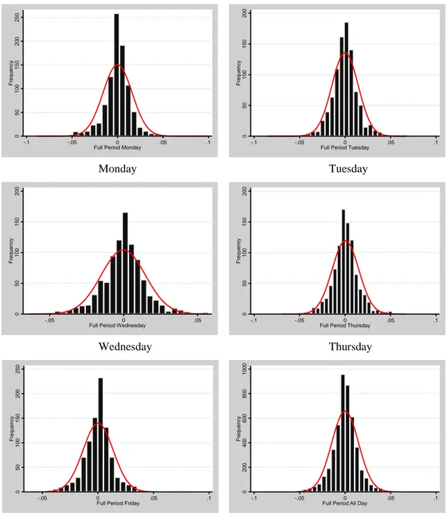
5.1

Descriptive Statistics

Figure iii: Histogram graphs fit with normal distribution for all weekdays and the full period

Source: Obtained from SPSS.

0 5 0 1 0 0 1 5 0 2 0 0 2 5 0 F re q u e n c y -.1 -.05 0 .05 .1

Full Period Monday

0 5 0 1 0 0 1 5 0 2 0 0 F re q u e n c y -.1 -.05 0 .05 .1

Full Period Tuesday

0 2 0 0 4 0 0 6 0 0 8 0 0 1 0 0 0 F re q u e n c y -.1 -.05 0 .05 .1

Full Period All Day

0 5 0 1 0 0 1 5 0 2 0 0 F re q u e n c y -.05 0 .05

Full Period Wednesday

0 5 0 1 0 0 1 5 0 2 0 0 F re q u e n c y -.1 -.05 0 .05 .1

Full Period Thursday

0 5 0 1 0 0 1 5 0 2 0 0 2 5 0 F re q u e n c y -.05 0 .05 .1

Full Period Friday

Monday Tuesday

Wednesday Thursday