Research
Evaluation of the simulation software
CIVA for qualification purpose
2017:29
Authors: Gustav Holmer Will Daniels Tommy Zettervall
SSM perspective
BackgroundModeling is an important tool within NDT, partly to develop and optimize
testing technologies, but also within the Qualification Body’s activities
to assess technical verifications and perform parameter studies. SSM has
supported university research in the area for many years and, among other
things, in the development of a software for ultrasound modeling. In
addi-tion, the accredited NDE laboratories are increasingly using software for
modeling inspection situations.
CIVA, developed by French CEA, is the commercially most successful
software in simulation of NDT situations. The program according to
the supplier can handle different materials, geometries, cladding and
anisotropy in arbitrary symmetry and orientation. Even simulation of
material structures, different probe types and defects with arbitrary
shape, size and orientation can be simulate. UT, ET and RT are the NDT
methods that the program can simulate. A project was started to evaluate
the usability of the software within qualification projects.
The work performed within this research report only handles with the
UT-module of the simulation software. The intended purpose with CIVA is
to provide a tool for developing and optimizing probe design, enhancing
qualification and supply help in analysis of inspection results.
The work has been carried out as collaboration between SQC (Swedish
Qualification Body) and AMEC.
Objective
The purpose of this project has been to evaluate the usability of the
simulation software CIVA within qualification projects.
CIVA software is used more and more in connection with qualification
of NDT inspection systems, both during technique development and
as a part of the technical justifications. The Qualification Body has to
know the boundaries of such simulation tool to be able to assess the
simulation results presented in a technical justification. Other areas
where the Qualification Body can use this simulation tool (if verified)
are parameter studies. Parameter studies can be used for review of
important parameters, in order to find out limit values as well as which
parameters are most important for the inspection system. In addition,
optimization of defect content for the manufacture of test blocks can
be done.
Results
The results of the work performed in this project indicate that
simula-tions and experiments matches rather well.
The largest discrepancy between the simulations and experiments
is noise or rather signal to noise ratio. Noise caused by the material
structure can be modelled in CIVA but as a separate layer, which is
super positioned on top of the defect response simulation, meaning
that the defect response is not affected by the noise. If a noise
simu-lation is used, it must be used together with additional attenuation
modeling or else the result will be a non-conservative signal to noise
ratio for any given indication. No simulations of noise or attenuation
were made within this project.
It is not possible to simulate a complete inspection, or validate an
inspection procedure by simulations with CIVA at the current time.
Both the producer of simulated data and the evaluator must have great
knowledge about the CIVA software to be able to draw the right
conclu-sions from the results. Whether CIVA can be used in qualifications or
not is a question of the purpose of the simulation and also the extent
of the usage of simulated data.
Need for further research
Noise is a significant part of a qualified procedure and the corresponding
technical justification. Defects responses are often evaluated in relation to
the surrounding noise levels rather than an arbitrary reference target, such as
a notch or SDH. Future work needs to be done focusing in CIVA capability
to simulate noise and attenuation.
Project information
Contact person SSM: Giselle García Roldán
Reference: SSM2010-299, 2037031-03
2017:29
Authors: Gustav Holmer1), Will Daniels2), Tommy Zettervall1)1) SQC Swedish Qualification Centre, Täby Sweden
2) AMEC Foster Wheeler, Birchwood, United Kingdom
Evaluation of the simulation software
CIVA for qualification purpose
This report concerns a study which has been conducted for the
Swedish Radiation Safety Authority, SSM. The conclusions and
view-points presented in the report are those of the author/authors and
do not necessarily coincide with those of the SSM.
Table of contents
List of abbreviations ... 2 1. Introduction ... 3 Purpose ... 3 Implementation ... 4 2. CIVA ... 5Identification of Regions of Applicability Stated in User Guide ... 5
Good Practice ... 8
EXTENDE Website ... 8
3. Ultrasonic equipment ... 8
4. Error analysis ... 9
Anticipated errors ... 10
Error due to Digitization ... 10
Other Quantifiable Errors ... 11
Other Errors ... 12
CIVA Internal Parameters ... 12
5. Experiments and simulations... 13
Phase 1 experiments ... 13 Task 1 ... 13 Task 2 ... 16 Task 3 ... 18 Task 4 ... 19 Task 5 ... 23 Task 6 ... 25 Task 7 ... 27 Conclusions Phase 1 ... 29 Phase 2 experiments ... 29 Task 1 ... 30 Task 2 ... 31 Task 3 ... 34 Task 4 ... 35 Conclusions Phase 2 ... 38 Phase 3 experiments ... 38 Task 1 ... 38 Task 2 ... 39
RAYTRAIMnot in the list/CIVA Comparison Exercise ... 44
Conclusions Phase 3 ... 46
Phase 4 experiments ... 46
Experimental work ... 47
Morphology Extraction Process Applied to Stress Corrosion Crack Samples ... 47
Results and comparison ... 49
Echo prediction discussion ... 50
Conclusions Phase 4 ... 51
Phase 5 experiments ... 51
Conclusions phase 5 ... 53
6. Conclusions ... 54
List of abbreviations
Abbreviation Explanation
AMEC
BAM Amec Foster Wheeler plc Bundesanstalt für Materialforschung und –prüfung
B-Scan Graphic presentation of UT-data as a side view
CAD Computer Aided Design
CEA Commissariat à l'énergie atomique
D/A Digital / Analog
EDM Electric Discharge Machining
ET Eddy Current Testing
FBH Flat Bottomed Hole
GTD Geometrical Theory of Diffraction
HIP Hot Isostatic Pressure
ISI In Service Inspection
MOD Ministry of Defence
NDE Non Destructive Evaluation
NDT Non Destructive Testing
NPP Nuclear Power Plant
PA Phased Array
PCS Probe Centre Separation
PE Pulse Echo
POD Probability of Detection
RT Radiographic Testing
SCC Stress Corrosion Crack
SDH Side Drilled Hole
SG Steam Generator
SKI Statens KärnkraftsInspektion
SOV Separation of Variables
SQC Swedish Qualification Centre AB
SSM Swedish Radiation Safety Authority
TOFD Time Of Flight Diffraction
TRL Transmit Receive Longitudinal
UK United Kingdom
UT Ultrasonic Testing
VTT Technical Research Centre of Finland
1. Introduction
Purpose
The purpose of this report and the work leading to it has been to evaluate the usabil-ity of the simulation software CIVA within qualification projects. Simulation soft-ware are used more and more as a tool during technique development and a part of technical justifications. In order to be able to assess the statements given as a result of simulations in a technical justification one has to know the boundaries of the simulation tools´ reliable performance. The work resulting in this report has been carried out with CIVA as it is the commercially most successful software and there-by the one most likely to appear in qualification documentation.
Nondestructive testing and evaluation in nuclear power plants differ from inspec-tions in the conventional industry in regard to the defects that are sought, and also the actions following when a defect is found. When a defect is found in conventional industry the object that is flawed is repaired and re-inspected. Once a weld is con-sidered free from defects it is generally not inspected again due to the fact that after manufacturing the risk of cracks decrease significantly. As repairs are very costly in nuclear power plants and the cost of a component failure even higher objects critical to plant safety are subject to periodic inspections. These inspections are designed to detect, size and characterize defects of different types with different characteristics in order to be able to assess the remaining life of the component before the defect becomes critical and a repair has to be made. These cracks with known damage mechanisms are typically harder to detect and characterize than typical manufactur-ing defects sought in conventional industry.
The intention of the verification process is to devise and apply a series of tests which can be used to:
• estimate the likely accuracy of the model prediction; • reach a view on the regions of applicability of the model
In general terms it can be expected that any model will have a region of problem space where its founding theory and assumptions are valid, a region where assump-tions are starting to be breached and a region where it should not be applied. This concept is shown in Figure 1.
Implementation
The work has been carried out as collaboration between SQC and AMEC, sponsored by SSM and MOD respectively. The general idea has been to identify a number of specific cases relevant to qualification work and set up a series of experiments on specimens with various shapes and reflectors with corresponding simulation runs. The results are then compared in terms of amplitude, echo dynamic and signal ap-pearance. Various types of signals that are common in ultrasonic inspections have been investigated, such as corner trap responses, tip diffraction (both TOFD and PE), Rayleigh waves and SDH and FBH specular reflection. Several different probes have been used.
The model verification activities are divided into five different partial phases. Each phase is divided into a number of different tasks with specific purposes. The exper-iments are described in detail in the Experexper-iments and simulations chapter. After completion of each phase a phase report has been produced that summarizes the obtained results, but no conclusions were presented in these reports. It was decided to draw the conclusions after the whole body of work was completed, to inaugurate the whole picture. However, when larger issues have occurred, some significant work has been carried out in order to find the root cause of the issue.
Model capability to be assessed
Phase 1 Response prediction for simple/smooth defects in simple materials and
probe modeling
Phase 2 Geometry handling with model
Phase 3 Complex materials – austenitic welds, inconels, dissimilar metal welds
Phase 4 Rough defects in simple materials
Phase 5 Rough defects in complex materials
Table 1 Comparison phases
The difference between simple/smooth defects and rough defects stated in Table 1 is that simple/smooth defects are typically artificial defects or an ideal fatigue crack. Rough defects are the type of defects that are typically service induced, with a clear morphology, following grain structure or other irregularities. By simple materials means carbon steel or stainless parent material that shows isotropic behavior. Com-plex materials show anisotropic behavior with significant influence on the sound beam giving effects such as large scattering, beam deflection and increased noise. There are options within CIVA to model attenuation caused by the material, in addi-tion to the sound beam divergence. This attenuaaddi-tion can easily be measured if your samples´ geometry will allow it and two identical probes can be used. This presents an issue also mentioned in chapter 3, Ultrasonic equipment. When it comes to noise and specifically grain noise caused by coarse grain structure and anisotropic materi-als it can materi-also be modelled if the grain structure is known and defined in CIVA.
However, this noise caused by the material structure is modelled as a separate layer which is super positioned on top of the defect response simulation, meaning that the defect response is not affected by the noise. If a noise simulation is used, it must be used together with additional attenuation modeling as mentioned above or else the result will be a non-conservative signal to noise ratio for any give indication. Because of the issues with noise and attenuation, no consideration of these phenom-ena has been taken within this project.
2. CIVA
CIVA is a software for simulation of NDT developed by the CEA. The software is capable of simulating UT, ET and RT. The work presented within this report only handles with the UT-module. The intended purpose with CIVA is to provide a tool for developing and optimizing probe design, enhancing qualification and supply help in analysis of inspection results.
When the work leading to this report was started CIVA version 9 was used. Since then version 10 and 11 has been released. This has raised questions concerning whether early simulation results are still valid at the time of publication of the re-sults. To some extent, this has been handled with reruns using CIVA version 11 for selected simulations. No large differences in the result were found, so it was decided that older simulations could be kept without any further action. However, if some errors in older simulations have been found, the new and rectified simulation has always been made with the latest version of the software.
Identification of Regions of Applicability Stated in User
Guide
In the user guidance supplied with CIVA version 11 [1], there is some discussion of regions of applicability. The following are extracts from the user guide text: Section 2.1.1.4, page 217: UT beam computation in welds and very
heterogene-ous media:
“… wavelength of the ultrasonic field has to be small when compared with some characteristic length of the model. Failure to comply can make the calculation unre-liable.”
A process for overcoming this problem is mentioned if not described.
On page 230 concerning the computation of the incident field, it is stated that the sound field is incompletely modelled in the transducer’s acoustic near field. Page 235: Main advantages and limitations of the Kirchoff’s [sic]
approxima-tion:
“Kirchhoff’s approximation is a high frequency approximation, valid when the de-fect is greater than the wavelength, that is, when ka >>1, where k is the wave-number and a is the main dimension of the defect.”
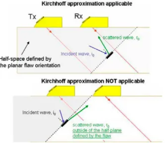
“The computation of this approximation implicitly assumes that both the transmitter and the receiver belong to the same half-space limited by the defect plane: the inci-dence and observation angle shall lie in the same side of the flaw, as illustrated on the following figure for a Tandem configuration:
For the first position (top of the figure), both probes are lying on the same side of the flaw, an echo is calculated. For the second position (bottom of the figure), the axis of the receiving probe doesn’t lie in the half space defined by the flaw orienta-tion, therefore one cannot predict the echo scattered by the flaw because the Kirch-hoff developed model is not applicable (the receiving probe is lying in the so-called 'shadowed area'). “
Figure 2 Limitation of Kirchoff model application using two probes in Tandem mode
“Similar limitations occur when using a pair of probes in TOFD inspection (see following figure) for nearly vertical flaws: The Kirchhoff model will soon be not applicable as the orientation of the flaw prevents the axis of the transmitter and receiver probes lying from the same side of the flaw. On the following figure, only the configuration displayed on top can be simulated using the Kirchhoff model.”
Figure 3 Limitation of Kirchoff application using two probes in TOFD mode
“The Kirchhoff approximation, classically used in NDT modelling, is assumed to give accurate results when the flaw is detected in specular or pseudo-specular mode, i.e. when the observation angle (the angle of the receiver) is close to the “natural” specular reflexion of the incidence wave upon the flaw.”
And later on page 237
“The Kirchhoff approximation is, therefore, mostly valid for:
- Specular reflexion over planar or volumetric defects, large compared to the wavelength (large ka, k being the wavenumber and a the characteristic length of the scatterer)”
and on page 238 regarding the corner effect model,
“Tip diffraction echoes from planar defects can be accurately predicted using the Kirchhoff approximation in terms of time of flight, however their amplitudes cannot be quantitatively predicted using the Kirchhoff model. The quantitative error is expected to increase when the scattered direction moves away from the specular direction.”
On page 239 regarding GTD
“GTD is also a high frequency approximation, valid when the defect is greater than
the wavelength, that is, when ka >>1, where k is the wave number and a is the main dimension of the defect.”
On page 265
“Limitations related to the use of superposition and modelled modes are recounted. In summary, the stated limitations are that the Kirchoff and GTD algorithms are suited to calculation of ultrasonic responses for defects which are large compared to the insonifying ultrasound’s wavelength and that the calculations are not reliable for defects in the transducer’s near field.”
Good Practice
The user guide contains a flow diagram, which is presented as good practice for safety critical application assessment as follows:
Figure 4 CIVA use best practice
In summary, the stated best practice requires users to examine the validation data sources which are identified as available publications, the provider’s website, or the user’s own experience for relevant validation information. In the event that no rele-vant data, it is suggested that the user obtains validation data through “specific ex-perimental validation”.
EXTENDE Website
EXTENDE (CIVA’s supplier, www.extende.com) maintain a website of validation evidence. The website contains a significant volume of validation work, but does not treat all information relevant to all possible cases of interest within nuclear power plant inspection design and qualification.
3. Ultrasonic equipment
Physical experiments have been carried out both at AMEC and SQC facilities using the following different UT-systems.
UT Hardware used UT Software Task
Phase 1 Peak NDT Micropulse 5 Arraygen Zetec Z-Scan UT UltraVision 1.1Q3 7 1-6
Phase 2 Zetec Z-Scan UT UltraVision 1.1Q3 1-6
Phase 3 Zetec Z-Scan UT
Zetec Dynaray Lite UltraVision 1.1Q3 UltraVision 3.3R4
Phase 4 Peak NDT Micropulse 5 N/A
Phase 5 Peak NDT Micropulse 5 N/A
Table 2 Ultrasonic equipment
Several different probes were used in the experiments. The probes that were used were chosen with the purpose of the experiment, geometry and material properties in the sample in mind. A limiting factor of probe choice is the amount of available probes available in SQC´s and AMEC´s laboratories. The result is that in all cases an optimal probe for the task may not have been used. The purpose is to compare simulations with experiments, not to obtain the best possible inspection result. Un-fortunately the limited selection of probes left the measurement of the samples at-tenuation impossible.
Probes used Type
Phase 1 TRC PCS 30 SWK 45-2 SWK 60-2 SWK 70-2 TRL 45-2 TRL 70-2
64 Element linear array
TOFD
Single crystal angle beam, Shear Single crystal angle beam, Shear Single crystal angle beam, Shear Dual crystal angle beam, Long Dual crystal angle beam, Long Phased array Phase 2 MWK 45-2 MWK 60-2 MWB 45-4 TRL 45-2 QCX 36 QCX 45 Wedge 45
Single crystal angle beam, Shear Single crystal angle beam, Shear Single crystal angle beam, Shear Dual crystal angle beam, Long Single crystal angle beam, Long Single crystal angle beam, Shear Single crystal angle beam, Shear Phase 3 TRL45-2 TRL60-2
TRL70-2
Dual crystal angle beam, Long Dual crystal angle beam, Long Dual crystal angle beam, Long Phase 4 45°S 60°S Single crystal angle beam, Shear Single crystal angle beam, Shear Phase 5 TRL45-2 TRL60-2 Dual crystal angle beam, Long Dual crystal angle beam, Long
Table 3 Ultrasonic probes
4. Error analysis
Data collection was controlled by a procedure authored by SQC and reviewed by AMEC. In what follow amplitude data are reported with respect to a pre-defined side drilled hole reference or geometrical feature of the sample as described in the data collection procedure specific for each experiment.
Anticipated errors
In order to assess the correlation between measured and modelled inspection data, it is necessary to quantify the sensitivity of the response to inspection parameter toler-ances. For instance, the defect through wall extent, beam angles, pulse shape, fre-quency, while controlled, are only known to certain tolerances. The measured data are obtained with equipment parameters and from samples for which the specifica-tion is only known to certain tolerances.
An assessment has been performed to establish the likely sensitivity of the modelled result to the likely parameter tolerances. This gives a means for comparing measured and modelled data, and judging the significance of any discrepancies.
The method used was firstly to identify influential parameters, and then evaluate the likely tolerance and concomitant amplitude variation associated with each parame-ter. The variations were then combined using a partial Monte Carlo error combina-tion approach.
Error due to Digitization
The analogue response signal is digitized in the experimental data used in this study. The digitization is at uniform time steps with discrete amplitude quantization. Two equipment systems have been used in this study. The PE and TOFD system had a 12-bit amplitude resolution and a digitization frequency of 50 MHz.
It means that the amplitude is sampled every 1/(50x106 ) seconds and that the
equipment’s full-scale is sampled in 212 increments. In this experimental
pro-gramme, phase information is maintained. So one amplitude bit is effectively sacri-ficed to record the phase (bipolar digitization), so that the amplitude is resolved to 1/211 of the equipment’s D/A converter full scale. In practice, this means a
possibil-ity of underestimating the signal response by up to one amplitude quantization step or one part in 2048. In a regime where the full-scale is set sensibly, this error is vir-tually negligible.
Waveform sampling means there is a tendency to underestimate the amplitude. The digitization error is proportional to the sampling interval and the probe frequency. An approximation of this error, assuming that the measured quantity is always a peak in response, can be obtained on a worst case basis as follows:
1. Assume that the response waveform in the vicinity of the peak has the form:
A= A0.sin(ωt+σ)
Where A0 is thepeak amplitude, ω is the probe’s (central) angular frequency, t is
time and σ is the phase angle.
2. Assume that the peak condition, where sin(ωt+σ)=1, falls exactly between discrete clock times. Thus the peak measurement would be A=
A0.sin(π/2+ω.Δt) where Δt is the sampling interval (1/digitization
frequen-cy). For a 5MHz probe and a 50MHz digitization frequency, the maximum undersize would be about 20% of the peak.
Other Quantifiable Errors
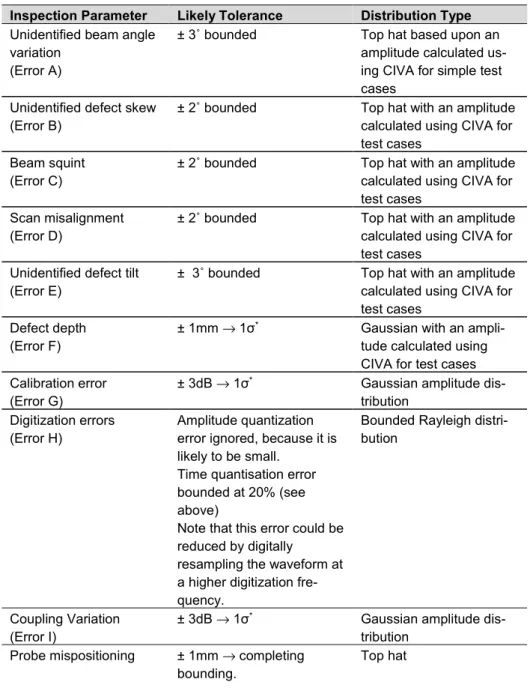
The other quantifiable errors in probe and defect specification contributing to the total error in amplitude are summarized in Table 4.
Inspection Parameter Likely Tolerance Distribution Type
Unidentified beam angle variation
(Error A)
± 3˚ bounded Top hat based upon an
amplitude calculated us-ing CIVA for simple test cases
Unidentified defect skew
(Error B) ± 2˚ bounded Top hat with an amplitude calculated using CIVA for
test cases Beam squint
(Error C) ± 2˚ bounded Top hat with an amplitude calculated using CIVA for
test cases Scan misalignment
(Error D) ± 2˚ bounded Top hat with an amplitude calculated using CIVA for
test cases Unidentified defect tilt
(Error E) ± 3˚ bounded Top hat with an amplitude calculated using CIVA for
test cases Defect depth
(Error F) ± 1mm → 1σ
* Gaussian with an
ampli-tude calculated using CIVA for test cases Calibration error
(Error G) ± 3dB → 1σ
* Gaussian amplitude
dis-tribution Digitization errors
(Error H) Amplitude quantization error ignored, because it is likely to be small.
Time quantisation error bounded at 20% (see above)
Note that this error could be reduced by digitally
resampling the waveform at a higher digitization fre-quency.
Bounded Rayleigh distri-bution
Coupling Variation
(Error I) ± 3dB → 1σ
* Gaussian amplitude
dis-tribution
Probe mispositioning ± 1mm → completing
bounding. Top hat
Table 4 Uncertainties contributing to overall amplitude error. The bulk of the
ampli-tude data ranges have been estimated from simple runs of CIVA using small varia-tions in individual parameters. *Note that σ in this table is standard deviation, and not phase angle as stated in ‘error due to digitization’
The general method in error calculation is to associate a distribution of error for each of the identified quantities listed above. Then for a single realization of possible errors, a realization of each source error (An..In) according to the distribution
func-tion is made and combined as follows:
Errorn= Error An + Error Bn+………+Error In
A large number (typically 10000) of such realizations are made and the statistics of the error distribution are assessed. It is this process which yields an assessment of likely errors.
Note that this approach to establishing credible errors in amplitude measurement is by its nature approximate in that it uses the model under test to establish the varia-tion in amplitude with likely uncertainty in key parameters affecting the response amplitude. Another approximation is that the typical values of parameters have been used, where in fact there would be dependence upon the exact parameters used for the specific case investigated. Despite these limitations, it is still useful to have a view on what would constitute an anticipated error.
Based upon a survey of sensitivity and application of the distribution functions de-scribed above using AMEC’s error combination calculation, a normally distributed error was obtained. The mean error was found to be close to zero, with some ten-dency to underestimate amplitude in most cases, and the standard deviation was nearly 6dB. Thus the experimental and modelled results would be expected to be usually within 6dB of one another.
Other Errors
In common with any experiment, not all the error sources which can contribute to the overall accuracy of the measurement are apparent. Of particular relevance in this study are features of targets which cannot be fully known. For example, defects can possess fine structure which may influence response amplitude in a complex man-ner, and which cannot be revealed without destructive examination.
CIVA Internal Parameters
CIVA has a number of internal parameters which can be set and can potentially affect the model output. It is for instance possible to select either Kirchoff or GTD modelling to describe the scattering process for planar targets, or Kirchoff and SOV for SDH. It is also possible to set a ‘quality’ parameter. Some testing of the sensi-tivity of the model output to optional features has been performed. The selection of the interactions in the models was determined by the advice obtained in the CIVA 10 manual. In some cases where responses are obtained that are not specific to the interaction selected i.e. obtaining edge diffracted (tip) signals from Kirchoff (specu-lar) interactions, an explanation of validity is given.
Figure 5 Regions of applicability for Kirchoff and GTD (taken from CIVA 10 manual)
Figure 5 shows where Kirchoff and GTD are applicable in relation to the orientation of the defect, with
α
=
0
representing a vertical flaw. This figure effectively illus-trates what is described in chapter 2. The Kirchoff approximation in CIVA gives rise to a tip response that is positioned correctly in terms of time of flight, but the ampli-tude may be inaccurate, with the error increasing with departure of the scatter direc-tion from specular.5. Experiments and simulations
Phase 1 experiments
Phase 1 concerned probe modeling and defect response from simple artificial defects and reflectors, such as common reference targets as SDH or notches or mechanical fatigue cracks in parent material. Also some work was done to test the models´ per-formance with TOFD and phased array applications.
Task 1
Task 1 concerned the collection and modelling of ultrasonic echo data collected from a series of lab-grown high-cycle mechanical fatigue cracks in stainless steel plate samples, referred to as SKI-plates or samples. The manufacturing process would be expected to generate defects which are relatively smooth faced and sharp tipped. These characteristics would tend to make the experimental data a good test of tip signal amplitude, reasonable test of corner response and signal appearance likeness. The cracks in these samples have since their manufacturing proven to be very tight and efforts have been made to increase their width with varying results. An effect of this can be seen in task 3, where signals are seen that wouldn’t be pre-sent if the defects were ideal.
Samples have been investigated which are 36mm thick with fatigue cracks including through wall extents of 10%, 20% and 50% of the plate thickness. The plates (20% & 50%) are similar to those used in “Experimental Validation of UTDefect, SKI
Report 97:3” [2], but in this case made of stainless steel instead of carbon steel. UTDefect is a simulation software developed at Chalmers University in Gothenburg, Sweden.
SKI Samples SS 36/3.6 SS 36/7.2 SS 36/18
Table 5 Samples used in Phase 1, task 1
The smallest defect, at 10% through wall extent, corresponds to a size of 3.6mm, which is at the limit of the validity of the models in Kirchoff and GTD. The models are only valid for when the defect extents are significantly greater than the wave-length.
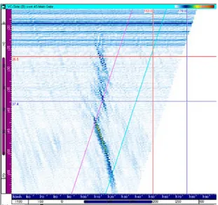
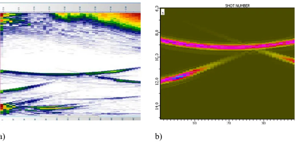
An example of the result is presented in Figure 6 below.
a) b)
Figure 645° TRL probe on 18 mm mechanical fatigue crack. a) showing experi-mental result and b) showing the simulated result. Amplitudes of tip signals within 4dB. Amplitudes of corner signals within 2dB
In the graph (Figure 7) below the distribution of simulated signal responses are shown in relation to the experimentally acquired response. It is important to note that the delta is calculated as follows:
Δ = predicted amplitude - measured amplitude.
Report 97:3” [2], but in this case made of stainless steel instead of carbon steel. UTDefect is a simulation software developed at Chalmers University in Gothenburg, Sweden.
SKI Samples SS 36/3.6 SS 36/7.2 SS 36/18
Table 5 Samples used in Phase 1, task 1
The smallest defect, at 10% through wall extent, corresponds to a size of 3.6mm, which is at the limit of the validity of the models in Kirchoff and GTD. The models are only valid for when the defect extents are significantly greater than the wave-length.
An example of the result is presented in Figure 6 below.
a) b)
Figure 645° TRL probe on 18 mm mechanical fatigue crack. a) showing experi-mental result and b) showing the simulated result. Amplitudes of tip signals within 4dB. Amplitudes of corner signals within 2dB
In the graph (Figure 7) below the distribution of simulated signal responses are shown in relation to the experimentally acquired response. It is important to note that the delta is calculated as follows:
Δ = predicted amplitude - measured amplitude.
The tip responses are separated in respect to simulation method (GTD or Kirchoff).
a)
b)
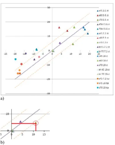
Figure 7 a) Comparison of experimental (horizontal) and CIVA predicted (vertical)
amplitude for opposite surface breaking fatigue crack defects of three depths(3,6, 7,2 and 18 mm) insonified with variety of probes. Amplitude data are presented for both crack tips. b) Example of reading the graph. The circled experiment measured +11dB and the corresponding simulation was + 5dB
In the majority of cases, the predictions are within 6dB of the experimental meas-urements. Largest discrepancies are for the:
• 60° shear corner trap on the 7.2mm defect where the amplitude predicted is significantly larger than was observed in measurement,
• 70° TRL 7.2mm and 3.6mm deep corner traps • 45° TRL 7.2mm corner trap
• 70° shear tip on 18mm defect
As all experiments didn´t show any tip signals the population in the tip measure-ments are not as big as for corner trap response. The reason that a significant amount (8 out of 15) tip responses cannot be seen is likely due to the fact that the signal is hidden within the signal from the corner trap or that the diffraction is too weak to be seen. Noise was not modeled in this application.
Corner trap Tip (Kirchoff) Tip (GTD)
Mean delta +2,6 dB +7,0 dB +2,5 dB
Task 2
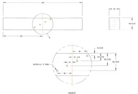
Task 2, pulse echo examination of reference side drilled holes, concerned data col-lection from a simple reference block (Figure 8) containing reference holes manu-factured from the same material grades and covering the depth range of interest in the SKI samples used in task 1. Again, blocks were scanned with the set of pulse echo probes identified for the project.
The SDH models were processed using Kirchoff and SOV, with the latter taking into account any creeping waves, which would be anticipated for 3mm side drilled holes given the frequency of the probes. Both calculations were conducted to determine how much improvement in the amplitude responses are seen when using SOV.
Task 2
Task 2, pulse echo examination of reference side drilled holes, concerned data col-lection from a simple reference block (Figure 8) containing reference holes manu-factured from the same material grades and covering the depth range of interest in the SKI samples used in task 1. Again, blocks were scanned with the set of pulse echo probes identified for the project.
The SDH models were processed using Kirchoff and SOV, with the latter taking into account any creeping waves, which would be anticipated for 3mm side drilled holes given the frequency of the probes. Both calculations were conducted to determine how much improvement in the amplitude responses are seen when using SOV.
Figure 8 SDH specimen
Figure 9 Comparison of experimental (horizontal) and CIVA predicted (vertical)
am-plitude for three depths of side drilled hole reference targets examined with a range of ultrasonic probes
The differences (delta amplitude) between the measured and predicted echo ampli-tude sets of results are good for the 5mm, 15mm and 25mm depth SDHs in shear wave mode. Results are also good for the 15mm and 25mm depth SDHs in the com-pression wave mode. The differences are within 3dB for the CIVA models run using Kirchoff but within 2dB for those run with SOV. However the results for the 5mm depth SDH show less good agreement for the 45° compression wave probe where an amplitude difference of greater than 10dB between measured and predicted peak amplitudes was recorded for both models run in Kirchoff and SOV (the CIVA result overestimated the measured result). This large mismatch would not be unexpected because the hole is at short range, well below the focal range of the probe and in a region likely to be poorly described by the model. Note also that the delta amplitude even for the 70° probe is better than 4dB. The results are presented in Figure 9. In general terms, the results shows that the response signals for the side drilled holes within the probes’ focal range zones are well predicted by CIVA, but that for the shortest beam paths, the mismatch between measurement and CIVA prediction is larger (>10dB peak amplitude error). This indicates that, as might be expected, modelling of scattering for targets outside the probes’ focused region is less well matched with measurement than for targets close to or within the focal range of the probes.
These results can be compared to the validation data presented on Extende´s (suppli-er of the software) web site [4] that presents a similar study. The results compare relatively well. However, the Extende validation data shows even better amplitude estimations from CIVA. The reason for this may be how the test was performed and as the experimental setup is unknown, the results are not directly comparable.
Task 3
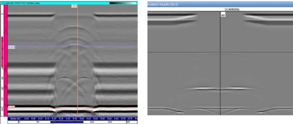
The third task dealt with limited application of time of flight scanning to the SKI sample set. To this end, the 50% defect (18mm fatigue crack) was scanned using 30° probes from both sides of the sample as illustrated in Figure 10. To clarify nomen-clature, near side scanning refers to scanning from position (A) and the far side from position (B). Near and far is referring to the crack opening.
Figure 10 TOFD scanning setup
As amplitude is not of great importance when evaluating TOFD data no analysis of the predicted amplitudes was made. It was noted though that the predicted signal amplitudes are within 4dB of the experimental case. What is important when evalu-ating TOFD data is the timing of the signals and the phase response of the different echoes and diffraction signals, so these properties has been evaluated.
The comparison that can be made consists of assessment of: • Relative phasing;
• Arc shape and general appearance; • Timing;
• Relative amplitude – qualitative.
Figure 11 Near side experimental scan and simulation
The results in Figure 11 show the response from the defect from the near side. The main signals’ phase relationship in the experiment and model are the same. There is however additional signals in the experimental results not present in the modelled
Task 3
The third task dealt with limited application of time of flight scanning to the SKI sample set. To this end, the 50% defect (18mm fatigue crack) was scanned using 30° probes from both sides of the sample as illustrated in Figure 10. To clarify nomen-clature, near side scanning refers to scanning from position (A) and the far side from position (B). Near and far is referring to the crack opening.
Figure 10 TOFD scanning setup
As amplitude is not of great importance when evaluating TOFD data no analysis of the predicted amplitudes was made. It was noted though that the predicted signal amplitudes are within 4dB of the experimental case. What is important when evalu-ating TOFD data is the timing of the signals and the phase response of the different echoes and diffraction signals, so these properties has been evaluated.
The comparison that can be made consists of assessment of: • Relative phasing;
• Arc shape and general appearance; • Timing;
• Relative amplitude – qualitative.
Figure 11 Near side experimental scan and simulation
The results in Figure 11 show the response from the defect from the near side. The main signals’ phase relationship in the experiment and model are the same. There is however additional signals in the experimental results not present in the modelled
results. These signals were discussed in chapter “Task 1” where the SKI samples were introduced.
Figure 12 Far side experimental scan and simulation
Generally these signals are secondary to the main features necessary to detect and size the defect. The phase between the lateral wave and back wall appear to have the expected 180° phase difference in both the experiment and CIVA. Where relevant comparisons can be made, for the signals present in both images, the arrival times of the tip signal are very similar in both experiment and CIVA prediction. It is possible to shift the phase of the ultrasonic pulse in CIVA to better match the appearance of the signals of the experiment. This was not done as only the relative phases of the different signals are of interest.
The far side experimental data (Figure 12) do not show the multiple tips found in the near side scans. There are a variety of possible explanations for this ranging from fine structure of the defect through to the relative strength of the diffraction coeffi-cient for the two sets of extreme incidence conditions.
There is TOFD validation data on the suppliers´ web site [4]. It is explained that the CIVA model is not very accurate regarding amplitude with probes that have band-widths above 80%. This correlates well with our observations. It is important to remember that a high bandwidth is desirable in TOFD applications to ensure as large beam spread a possible.
Task 4
The fourth task compared model and experimental data collected from a series of FBHs when examined with pule echo probes from the probe set.
The comparison between experiment and simulations that can be made consists of assessment of:
• Echo dynamic appearance / pattern recognition • Amplitude
An example of experiment versus simulation is shown in Figure 13 below. Note that no back wall reflection was simulated and are not present in the simulated B-scan. The simulated B-scan also shows an overlay of the test specimen.
Figure 13 Measured and simulated B-scans for inclined FBH targets
The overlay has given very interesting information, as it has shown that when using higher angle probes, the data seems to be displaced. An example of this is shown in Figure 14 below.
Figure 14 Displacement of Maximum amplitude with depth (70° compression) for
FBHs
The displacement of signals is also present if the simulated data from Task 2 is pre-sented with an overlay. See Figure 15.
Figure 15 Displacement also present on SDH-data (70° compression)
The reason for this misplacement is not fully investigated.
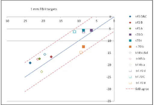
Figure 16 Comparison of experimental (horizontal) and CIVA predicted (vertical)
amplitude for 1 mm FBH targets examined with a range of ultrasonic probes
In this case (Figure 16), all predicted responses were within ±6dB. In general the 70° responses were of higher amplitude than the 45° responses.
Figure 17 Comparison of experimental (horizontal) and CIVA predicted (vertical)
amplitude for 2 mm FBH targets examined with a range of ultrasonic probes
For the bulk of the cases examined (presented in Figure 17), predictions and meas-urements were within 6dB. Largest differences exist for the 70° TRL probe at short range and the 70° conventional shear wave probe examining the deepest FBH.
Figure 18 Comparison of experimental (horizontal) and CIVA predicted (vertical)
amplitude for 3 mm FBH targets examined with a range of ultrasonic probes
As for the previous plot (Figure 18), the difference between the measured and calcu-lated amplitudes for the majority of cases is within 6dB. As observed in the previous
plot, the largest differences occur for the shallowest holes (C&D) observed with the 70° TRL probe and the deepest hole (A) insonified by the conventional 70° shear wave probe.
Task 5
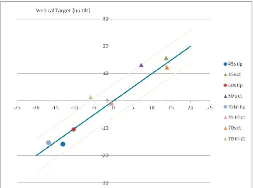
The fifth task investigated the prediction and experimental data for a range of sur-face breaking notches with tilt. The test specimens are presented in Figure 19 below. The notches were scanned from both directions, providing a test set with defects with tilts -20°, -10°, 0°, 10° and 20°. The scans were performed so that the notches were far surface breaking.
Figure 19 Test specimens task 5
The differences between simulated responses and experimental response amplitude are compiled in Figure 20. The mismatch between measurement and theory is quite large in some cases – in particular at 60˚ beam angle cases. The values in the graph are calculated as simulated amplitude – measured amplitude. The mean delta ampli-tude value is -3,8dB and the standard deviation comes out quite large at 6,5 dB.
Figure 20 Vertical 10mm slot showing tip and corner trap response for a variety of
probes
Figure 21 10° inclined 10mm slot showing tip and corner trap responses for a variety
of probes. The spread of results is larger than for a vertical slot. The CIVA model tends to under estimate the echo amplitude in these cases
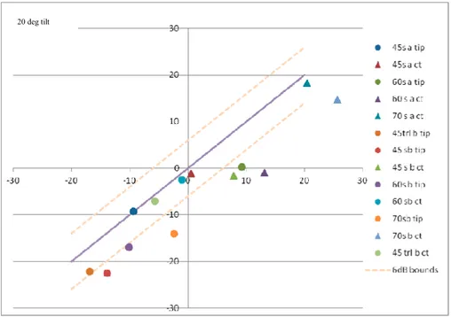
Figure 22 20° inclined 10mm slot showing tip and corner trap responses for a variety
of probes. Once again, the spread of results is larger than for the vertical case. The CIVA model tends to underestimate the echo amplitude where there is more signifi-cant error
Task 6
The sixth task investigated inspection of embedded planar defects with various con-figurations which are of interest for fabrication targets. Comparative results were only made between the first three sets of defects shown in Figure 23.
Figure 23 End view of embedded defects used in task 6
Below an example (Figure 24) of the signal response from defect 1 is shown when scanned with a 45°SWK probe.
Figure 24 Defect 1 experimental signal response
The experimental results showed that the upper tip signals for the shear wave probes have a smaller amplitude than the lower tip signals for both defects 1 and 2. The predicted responses show a high level of deviation from experimental observation for the higher angle probes. Response predictions from the UK Nuclear Utility simu-lation model PEDGE (UT simusimu-lation software) are included. The predictions made using this model are poorly matched with experiment too. It is suspected that much of the result here is linked to issues with the defect’s final form.
Figure 25 Comparison of experimental ( horizontal) and CIVA predicted (vertical)
amplitude for a circular vertical HIP´d target examined with a range of ultrasonic probes. Echoes are associated with the target tips labelled ‘u’ upper and ‘b’ bottom. Hollow triangles and boxes are run with UK model PEDGE
Figure 26 Comparison of experimental (horizontal) and CIVA predicted (vertical)
amplitude for an elliptical vertical HIP’d finns i listan redantarget examined with a range of ultrasonic probes. Echoes are associated with the target tips labelled ‘u’ upper and ‘b’ bottom
Task 7
In the seventh task, a 64 element phased array with a center frequency of 5MHz was used to investigate the basic phased array modelling capabilities within CIVA. The data collection activity was performed at AMEC using a Peak NDE Microplus 5 PA system.
In summary, two samples from the reference set were used in the investigation: • Reference block containing 3mm reference holes at depths of 5, 15, 25 and
35mm from the surface;
• 10mm vertical notch sample (as used in task 5). The reasons for using these two samples were that:
• the samples are relatively simple and both their form and the reflectors they contain are well defined,
• they provide a ready means for checking relevant beam-forming prediction capability, and
• the results correlate well with the modelling and experimental data collec-tion programme undertaken in the earlier stages of the project.
The Peak NDE Microplus 5 PA system is equipped with a delay law calculation tool (Arraygen), which produces delay laws in a file based form which can be imported into Microplus to configure the probe’s firing.
The delay law calculations were exported from Arraygen as a .MPS files and CIVA as .law files. For both sets of delay laws the figures produced were the same, or rather, the delay between each of the elements are identical. CIVA does appear to apply an offset at each angle of the sector scan but this has no effect on the delays between each element.
Table 7 shows the results from the corner trap and tip of the vertical notch. The 10mm vertical notch sample block (as used in task 5) was scanned experimentally from both sides (of the defect) and a mild asymmetry in results was observed which could arise from slight irregularities on the target or a small inclination or tilt angle. Options within CIVA have been used to select either the Kirchoff (default) or GTD tip response algorithms.
The amplitudes are reported with reference to a 3mm SDH at a depth of 40mm. The results show that there is less than 1dB difference between the experimental results for the corner tap response when scanned from two sides. Overall the modelled result is within 1.5dB of the experimental results. Figure 27 shows the experimental and modelled results as a B-scan image. In both sets of results the tip and corner signals can be clearly distinguished.
Table 7 Corner trap and tip responses from vertical notch
The tip signal amplitudes obtained from the experimental and modelled results show a larger difference than the corresponding corner response results (Table 7). The GTD model gives the lowest amplitude and this is more than 12dB lower than the amplitude obtained experimentally from side A. This result is probably explained by the slot having a relatively large width which acts as a reflector, whereas in the model the notch was represented by a slot with minimal width, which would give a lower amplitude response compared to a diffracted tip response.
a) b)
Figure 27B-scan images of the response from a vertical notch. a) showing experi-ment and b) showing simulation
The results from the reference hole calibrations are given in Table 8. The amplitude response differences between the modelled and experimental results are within 1dB for the hole at a depth of 15mm and within 1.5dB for the reference hole at 35mm. The calibration reference used in this configuration was a 3mm SDH at a depth of 25mm. The amplitude differences relative to the reference hole are small because of the unfocussed beam configuration however this is the case in the modelled and
Experimental
– Side A Experimental – Side B Kirchoff CIVA GTD
Corner Trap -0,7 dB -0,1 dB 0,5 dB N/A
Tip Signal -6,0 dB -7,8 dB -17 dB -20 dB
experimental results. The 5mm hole could not be scanned experimentally due to its proximity to the surface; hence no results are presented for this case.
Hole Depth Experiment CIVA
15 mm 1,3 dB 0,3 dB
35 mm -1,5 dB -0,1 dB
Table 8 Amplitude response from reference holes
a) b)
Figure 28 B-scan images from a 0-45° sectorial scan of a 25 mm depth 3 mm SDH.
a) showing experiment and b) showing simulation
The results from the phased array experiments has been in accordance with what has been seen in the other tasks, specular reflection and corner traps are modeled with good precision, but tip diffraction is usually not as accurate. As discussed above, this may be due to the differences in model and samples as well as less accurate model predictions.
Conclusions Phase 1
The trials performed in phase 1 largely resemble typical methods for calibration in qualified procedures. The specific UT methods (PE, PA and TOFD) assessed are also common in qualified inspection procedures.
As simulated amplitude response, phase and delay laws match the experimental results well this is a solid foundation to base more advanced simulations on.
Phase 2 experiments
Phase 2 handles complex geometries in simple (homogeneous and isotropic) materi-als. A set of test samples has been identified to contain a relevant set of geometries and reflectors. However, in some cases full knowledge of the manufacturing of the sample has not been known.
Task 1
The sample identified for task 1 is a forged alloy 403 reduction with three notches as shown in Figure 29.
Figure 29 Specimen 1.1_UT03
All available experimental scans of the complex geometry Specimen 1.1_UT03 (Figure 29) have been modelled. All scans have been modelled as half-skip consid-ering both longitudinal and transverse (shear) components and mode conversion. Initial studies made using CIVA 10 were incorrectly configured without a back wall, which meant skipped responses were not modelled as intended. When runs were repeated using CIVA 11, a warning was generated which enabled the fault to be rectified. Examples of B-scan results are shown in Figure 30.
a) Experimental measurement b) CIVA 11 prediction
Figure 30 Comparison of experimental measurement (a) and CIVA prediction (b) in
B-scan display. CIVA prediction made using CIVA 11
Scan 2 Scan 1