Equivalence Testing and the Second
Generation P-Value.
Daniël Lakens
Eindhoven University of Technology, The Netherlands
Marie Delacre
Université Libre de Bruxelles, Belgium
Abstract
To move beyond the limitations of null-hypothesis tests, statistical approaches have been developed where the ob-served data are compared against a range of values that are equivalent to the absence of a meaningful effect. Spec-ifying a range of values around zero allows researchers to statistically reject the presence of effects large enough to matter, and prevents practically insignificant effects from being interpreted as a statistically significant differ-ence. We compare the behavior of the recently proposed second generation p-value (Blume, D’Agostino McGowan, Dupont, & Greevy, 2018) with the more established Two One-Sided Tests (TOST) equivalence testing procedure (Schuirmann, 1987). We show that the two approaches yield almost identical results under optimal conditions. Under suboptimal conditions (e.g., when the confidence interval is wider than the equivalence range, or when confidence intervals are asymmetric) the second generation p-value becomes difficult to interpret. The second gen-eration p-value is interpretable in a dichotomous manner (i.e., when the SGPV equals 0 or 1 because the confidence intervals lies completely within or outside of the equivalence range), but this dichotomous interpretation does not require calculations. We conclude that equivalence tests yield more consistent p-values, distinguish between datasets that yield the same second generation p-value, and allow for easier control of Type I and Type II error rates.
Keywords: equivalence testing, second generation p-values, hypothesis testing, TOST, statistical inference
To test predictions researchers predominantly rely on null-hypothesis tests. This statistical approach can be used to examine whether observed data are sufficiently surprising under the null hypothesis to reject an effect that equals exactly zero. Null-hypothesis tests have an important limitation, in that this procedure can only re-ject the hypothesis that there is no effect, while scien-tists should also be able to provide statistical support for
equivalence. When testing for equivalence researchers
aim to examine whether an observed effect is too small to be considered meaningful, and therefore is
practi-cally equivalent to zero. By specifying a range around the null hypothesis of values that are deemed practically equivalent to the absence of an effect (i.e., 0 +- 0.3) the observed data can be compared against an
equiv-alence range and researchers can test if a meaningful
effect is absent (Hauck & Anderson, 1984; Kruschke, 2018; Rogers, Howard, & Vessey, 1993; Serlin & Lap-sley, 1985; Spiegelhalter, Freedman, & Parmar, 1994; Wellek, 2010; Westlake, 1972).
Second generation p-values (SGPV) were recently proposed as a statistic that represents “the proportion of
data-supported hypotheses that are also null hypothe-ses” (Blume et al., 2018). The researcher specifies an equivalence range around a null hypothesis of values that are considered practically equivalent to the null hypothesis. The SGPV measures the degree to which a set of data-supported parameter values falls within the interval null hypothesis. If the estimation inter-val falls completely within the equiinter-valence range, the SGPV is 1. If the confidence interval falls completely outside of the equivalence range, the SGPV is 0. Oth-erwise the SGPV is a value between 0 and 1 that ex-presses the overlap of data-supported hypotheses and the equivalence range. When calculating the SGPV the set of data-supported parameter values can be repre-sented by a confidence interval (CI), although one could also choose to use credible intervals or Likelihood sup-port intervals (SI). When a confidence interval is used, the SGPV and equivalence tests such as the Two One-Sided Tests (TOST) procedure (Lakens, 2017; Meyners, 2012; Quertemont, 2011; Schuirmann, 1987) appear to have close ties, because both tests compare a confi-dence interval against an equivalence range. Here, we aim to examine the similarities and differences between the TOST procedure and the SGPV. We limit our anal-ysis to continuous data sampled from a bivariate nor-mal distribution. The TOST procedure also relies on the confidence interval around the effect. In the TOST procedure the data are tested against the lower equiva-lence bound in the first one-sided test, and against the upper equivalence bound in the second one-sided test (Lakens, Scheel, & Isager, 2018). For an excellent dis-cussion of the strengths and weaknesses of different fre-quentist equivalence tests, including alternatives to the TOST procedure, see Meyners (2012). If both tests sta-tistically reject an effect as extreme or more extreme than the equivalence bound, you can conclude the ob-served effect is practically equivalent to zero from a Neyman-Pearson approach to statistical inferences. Be-cause one-sided tests are performed, one can also con-clude equivalence by checking whether the 1-2×α confi-dence interval (e.g., when the alpha level is 0.05, a 90% CI) falls completely within the equivalence bounds. Be-cause both equivalence tests as the SGPV are based on whether and how much a confidence interval overlaps with equivalence bounds, it seems worthwhile to com-pare the behavior of the newly proposed SGPV to equiv-alence tests to examine the unique contribution of the SGPV to the statistical toolbox.
The relationship between p-values from TOST and SGPV when confidence intervals are symmetrical
The second generation p-value (SGPV) is calculated as: pδ=|I ∩ H0| |I| × max ( |I| 2 |H0| , 1 )
where I is the interval based on the data (e.g., a 95% confidence interval) and H0 is the equivalence range.
The first term of this formula implies that the second generation p-value is the width of the confidence inter-val that overlaps with the equiinter-valence range, divided by the total width of the confidence interval. The second term is a “small sample correction” (which will be dis-cussed later) that comes into play whenever the confi-dence interval is more than twice as wide as the equiva-lence range. To examine the relation between the TOST
p-value and the SGPV we can calculate both statistics
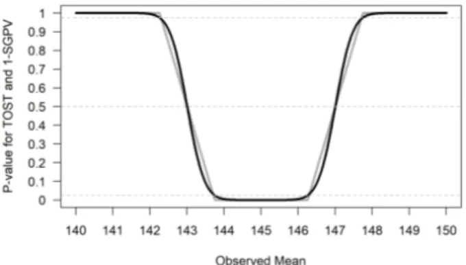
across a range of observed effect sizes. Building on the example by Blume et al. (2018), in Figure 1 p-values
are plotted for the TOST procedure and the SGPV. The statistics are calculated for hypothetical one-sample t-tests for observed means ranging from 140 to 150 (on the x-axis). The equivalence range is set to 145 +- 2 (i.e., an equivalence range from 143 to 147), the ob-served standard deviation is assumed to be 2, and the sample size is 30. For example, for the left-most point in Figure1the SGPV and the TOST p-value is calculated for a hypothetical study with a sample size of 30, an ob-served standard deviation of 2, and an obob-served mean of 140, where the p-value for the equivalence test is 1, and the SGPV is 0.
Our conclusions about the relationship between TOST values and SGPV hold for second generation p-values calculated from confidence intervals, and assum-ing data is sampled from a bivariate normal distribution. Readers can explore the relationship between TOST p-values and SGPV for themselves in an online Shiny app:
http://shiny.ieis.tue.nl/TOST_vs_SGPV/.
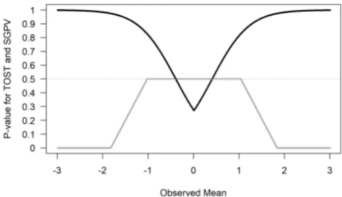
The SGPV treats the equivalence range as the null-hypothesis, while the TOST procedure treats the values outside of the equivalence range as the null-hypothesis. For ease of comparison we can plot 1-SGPV (see Figure
2) to make the values more easily comparable. We see that the p-value from the TOST procedure and the SGPV follow each other closely. When we discuss the relation-ship between the p-values from TOST and the SGPV, we focus on their correspondence at three values, namely where the TOST p = 0.025 and SGPV is 1, where the TOST p = 0.5 and SGPV = 0.5, and where the TOST
p = 0.975 and SGPV = 1. These three values are
im-portant for the SGPV because they indicate the values at which the SGPV indicates the data should be inter-preted as compatible with the null hypothesis (SGPV =
Figure 1. Comparison of p-values from TOST (black line) and SGPV (grey line) across a range of observed sample
means (x-axis) tested against a mean of 145 in a one-sample t-test with a sample size of 30 and a standard deviation of 2, illustrating that when the TOST p-value = 0.5, the SGPV = 0.5, when the TOST p-value is 0.975, 1-SGPV = 1, and when the TOST p-value = 0.025, 1-SGPV = 0.
1), or with the alternative hypothesis (SGPV = 0), or when the data are strictly inconclusive (SGPV = 0.5).
These three points of overlap are indicated by the horizontal dotted lines in Figure2at TOST p-values of 0.975, 0.5, and 0.025.
When the observed sample mean is 145, the sam-ple size is 30, and the standard deviation is 2, and we are testing against equivalence bounds of 143 and 147 using the TOST procedure for a one-sample t-test, the equivalence test is significant, t(29) = 5.48, p < .001. Because the 95% CI falls completely within the equiva-lence bounds, the SGPV is 1 (see Figure1). On the other hand, when the observed mean is 140, the equivalence test is not significant (the observed mean is far outside the equivalence range of 143 to 147), t(29) = -8.22,
p = 1 (or more accurately, p > .999 as p-values are
bounded between 0 and 1). Because the 95% CI falls completely outside the equivalence bounds, the SGPV is 0 (see Figure1).
SGPV as a uniform measure of overlap
It is clear the SGPV and the p-value from TOST are closely related. When confidence intervals are symmet-ric we can think of the SGPV as a straight line that is
Figure 2. Comparison of p-values from TOST (black
line) and 1-SGPV (grey line) across a range of observed sample means (x-axis) tested against a mean of 145 in a one-sample t-test with a sample size of 30 and a stan-dard deviation of 2.
directly related to the p-value from an equivalence test for three values. When the TOST p-value is 0.5, the SGPV is also 0.5 (note that the reverse is not true). The
Figure 3. Means, normal distribution, and 95% CI for
three example datasets that illustrate the relationship between p-values from TOST and SGPV.
SGPV is 50% when the observed mean falls exactly on the lower or upper equivalence bound, because 50% of the symmetrical confidence interval overlaps with the equivalence range. When the observed mean equals the equivalence bound, the difference between the mean in the data and the equivalence bound is 0, the t-value for the equivalence test is also 0, and thus the p-value is 0.5 (situation A, Figure3).
Two other points always have to overlap. When the 95% CI falls completely inside the equivalence region, and one endpoint of the confidence interval is exactly equal to one of the equivalence bounds (see situation B in Figure3) the TOST p-value (which relies on a one-sided test) is always 0.025, and the SGPV is 1. Note that when sample sizes are small or equivalence bounds are narrow, small p-values for the TOST or a SGPV = 1 might not be observed in practice if too few obser-vations are collected. The third point where the SGPV and the p-value from the TOST procedure should over-lap is where the 95% CI falls completely outside of the equivalence range, but one endpoint of the confidence interval is equal to the equivalence bound (see situation C in Figure3), when the p-value will always be 0.975, and the SGPV is 0. Note that this situation is in essence a minimum-effect test (Murphy, Myors, & Wolach, 2014). The goal of a minimum-effect is not just to reject a dif-ference of zero, but to reject the smallest effect size of interest (i.e., the equivalence bounds). An equivalence test and minimum effect test against the same equiva-lence bound are complementary, and when a TOST p-value is larger than 0.975, the p-p-value for the minimum effect test is smaller than 0.05 (and therefore the mini-mum effect test provides no additional information that can not be derived from the p-value from the
equiva-Figure 4. Means, normal distribution, and 95% CI for
samples where the observed population mean is 1.5, 1.4, 1.3, and 1.2.
lence test). The SGPV summarizes the information from an equivalence test (and the complementary minimum-effect test). These can be two relevant questions to ask, although it often makes sense to combine an equiva-lence test and a null-hypothesis test instead (Lakens et al., 2018).
For example, in Figure4we have plotted four SGPV’s. From A to D the SGPV is 0.76, 0.81, 0.86, and 0.91. The difference in the percentage of overlap between A and B (-0.05) is identical to the difference in the percentage of overlap between C and D as the mean gets 0.1 closer to the test value (-0.05). As the observed mean in a one-sample t-test lies closer to the test value, from situation A to D, the difference in the overlap changes uniformly. As we move the observed mean closer to the test value in steps of 0.1 across A to D the p-value calculated for normally distributed data are not uniformly distributed. The probability of observing data more extreme than the upper bound of 2 is (from A to D) 0.16, 0.12, 0.08, and 0.05. As we can see, the difference between A and B (0.04) is not the same as the difference between C and D (0.03). Indeed, the difference in p-values is the largest as you start at p = 0.5 (when the observed mean falls on the test value), which is why the line in Figure
1is the steepest at p = 0.5. Note that where the SGPV reaches 1 or 0, p-values closely approximate 0 and 1, but never reach these values.
When different p-values for equivalence tests yield the same SGPV
There are three situations where p-values for TOST differentiate between observed results, while the SGPV does not differentiate. The first two situations were discussed before and can be seen in Figure 1. When
Figure 5. The relationship between p-values from the
TOST procedure and the SGPV for the same scenario as in Figure1.
the SGPV is either 0 or 1, p-values from the equiva-lence test fall between 0.975 and 1 or between 0 and 0.025. Where the SGPV is 1 as long as the confidence interval falls completely within the equivalence bounds, the p-value for the TOST continues to differentiate be-tween results as a function of how far the confidence interval lies within the equivalence bounds (the further the confidence interval is from both bounds, the lower the p-value). The easiest way to see this is by plotting the SGPV against the p-value from the TOST procedure. The situations where the p-values from the TOST pro-cedure continue to differentiate based on how extreme the results are, but the SGPV is a fixed value are indi-cated by the parts of the curve where there are vertical straight lines at second generation p-values of 0 and 1.
A third situation in which the SGPV remains stable across a range of observed effects, while the TOST p-value continues to differentiate, is whenever the CI is wider than the equivalence range, and the CI overlaps with the upper and lower equivalence bound. When the confidence interval is more than twice as wide as the equivalence range the SGPV is set to 0.5. Blume et al. (2018) call this the “small sample correction factor”. However, it is not a correction in the typical sense of the word, since the SGPV is not adjusted to any “correct” value. When the normal calculation would be “mislead-ing” (i.e., the SGPV would be small, which normally would suggest support for the alternative hypothesis, but at the same time all values in the equivalence range are supported), the SGPV is set to 0.5 which according to Blume and colleagues signals that the SGPV is “un-informative”. Note that the CI can be twice as wide as the equivalence range whenever the sample size is small (and the confidence interval width is large) or when
Figure 6. Comparison of p-values from TOST (black
line) and SGPV (grey line) across a range of observed sample means (x-axis). Because the sample size is small (n = 10) and with a standard deviation of 2 the CI is more than twice as wide as the equivalence range (set to -0.4 to 0.4), the SGPV is set to 0.5 (horizontal light-grey line) across a range of observed means.
then equivalence range is narrow. It is therefore not so much a “small sample correction” as it is an exception to the typical calculation of the SGPV whenever the ra-tio of the confidence interval width to the equivalence range exceeds 2:1 and the CI overlaps with the upper and lower bounds.
We can examine this situation by calculating the SGPV and performing the TOST for a situation where sample sizes are small and the equivalence range is nar-row, such that the CI is more than twice as large as the equivalence range (see Figure6). When the two statis-tics are plotted against each other we can see where the SGPV is the same while the TOST p-value still differ-entiates different observed means (indicated by straight lines in the curve, see Figure 7). We see the SGPV is 0.5 for a range of observed means where the p-value from the equivalence test still varies. It should be noted that in these calculations the p-values for the TOST pro-cedure are never smaller than 0.05 (i.e., they do not get below 0.05 on the y-axis). In other words, we can-not conclude equivalence based on any of the observed means. This happens because we are examining a sce-nario where the 90% CI is so wide that it never falls completely within the two equivalence bounds.
As Lakens (2017) notes: “in small samples (where CIs are wide), a study might have no statistical power (i.e., the CI will always be so wide that it is necessarily wider than the equivalence bounds).” None of the p-values based on the TOST procedure are below 0.05, and thus, in the long run we have 0% power.
Figure 7. The relationship between p-values from the
TOST procedure and the SGPV for the same scenario as in Figure6.
The p-value from the TOST procedure still differen-tiates observed means, while the SGPV does not, when the CI is wider than the equivalence range (so the pre-cision is low) and overlaps with the upper and lower equivalence bound, but the CI is not twice as wide as the equivalence range. In the example below, we see that the CI is only 1.79 times as wide as the equivalence bounds, but the CI overlaps with the lower and upper equivalence bounds (Figure8). This means the SGPV is not set to 0.5, but it is constant across a range of ob-served means, while the TOST p-value is not constant across this range.
If the observed mean would be somewhat closer to 0, or further away from 0, the SGPV remains constant (the CI width does not change, and it completely
over-Figure 8. Example of a 95% CI that overlaps with the
lower and upper equivalence bound (indicated by the vertical dotted lines).
Figure 9. Comparison of p-values from TOST (black
line) and SGPV (grey line) across a range of observed sample means (x-axis). The sample size is small (n = 10), but because the sd is half as big as in Figure7(1 in-stead of 2) the CI is less than twice as wide as the equiv-alence range (set to -0.4 to 0.4). The SGPV is not set to 0.5 (horizontal light grey line) but reaches a maximum slightly above 0.5 across a range of observed means.
laps with the equivalence range) while the p-value for the TOST procedure does vary. We can see this in Fig-ure9below. The SGPV is not set to 0.5, but is slightly higher than 0.5 across a range of means. How high the SGPV will be for a CI that is not twice as wide as the equivalence range, but overlaps with the lower and up-per equivalence bounds, depends on the width of the CI and the equivalence range.
If we once more plot the two statistics against each other we see the SGPV is 0.56 for a range of observed means where the p-value from the equivalence test still varies, as indicated by the straight section of the line (Figure10).
To conclude this section, there are situations where the p-value from the TOST procedure continues to dif-ferentiate, while the SGPV does not. Therefore, inter-preted as a continuous statistic, the SGPV is more lim-ited than the p-value from the TOST procedure.
The relation between equivalence tests and SGPV for asymmetrical confidence intervals around correla-tions
So far we have only looked at the relation between equivalence tests and the SGPV when confidence inter-vals are symmetric (e.g., for confidence interinter-vals around mean differences). For correlations, which are bound between -1 and 1, confidence intervals are only symmet-ric for a correlation of exactly 0. The confidence inter-val for a correlation becomes increasingly asymmetric
Figure 10. The relationship between p-values from the TOST procedure and the SGPV for the same scenario as in
Figure9.
as the observed correlation nears -1 or 1. For example, with ten observations, an observed correlation of 0 has a symmetric 95% confidence interval ranging from -0.63 to 0.63, while and observed correlation of 0.7 has an asymmetric 95% confidence interval ranging from 0.13 to 0.92. Note that calculating confidence intervals for a correlation involves a Fisher’s z-transformation, which transforms values such that they are approximately nor-mally z-distributed, which allows one to compute sym-metric confidence intervals. These confidence intervals are then retransformed into a correlation, where the confidence intervals are asymmetric if the correlation is not exactly zero.
The effect of asymmetric confidence intervals around correlations is most noticeable at smaller sample sizes. In Figure11we plot the p-values from equivalence tests and the SGPV (again plotted as 1-SGPV for ease of com-parison) for correlations. The sample size is 30 pairs of observations, and the lower and upper equivalence bounds are set to -0.45 and 0.45, with an alpha of 0.05. As the observed correlation in the sample moves from -.99 to 0 the p-value from the equivalence test becomes smaller, as does 1-SGPV. The pattern is quite similar to that in Figure 2. The p-value for the TOST procedure and 1-SGPV are still related as discussed above, with TOST p-values of 0.975 and 0.025 corresponding to a
1-SGPV of 1 and 0, respectively. There are two important differences, however. First of all, the SGPV is no longer a straight line, but a curve, due to the asymmetry in the 95% CI. Second, and most importantly, the p-value for the equivalence test and the SGPV do no longer overlap at p = 0.5.
The reason that the equivalence test and SGPV no longer overlap is due to asymmetric confidence inter-vals. If the observed correlation falls exactly on the equivalence bound the p-value for the equivalence test is 0.5. In the equivalence test for correlations the p-value is computed based on a z-transformation which better controls error rates (Goertzen & Cribbie, 2010). This transformation is computed as follows, where r is the observed correlation and ρ is the theoretical corre-lation under the null:
z= log(1+r1−r) 2 − log(1+ρ1−ρ) 2 q 1 n−3
Because the z-distribution is symmetric, the probabil-ity of observing the observed or more extreme z-score, assuming the equivalence bound is the true effect size, is 50%. However, because the r distribution is not sym-metric, this does not mean that there is always a 50% probability of observing a correlation smaller or larger
Figure 11. Comparison of p-values from TOST (black
line) and 1-SGPV (grey curve) across a range of ob-served sample correlations (x-axis) tested against equiv-alence bounds of r = -0.45 and r = 0.45 with n = 30 and an alpha of 0.05.
Figure 12. Three 95% confidence intervals for observed
effect sizes of r = -0.45, r = 0, and r = 0.45 for n = 30. Only the confidence interval for r = 0 is symmetric.
than the true correlation. As can be seen in Figure12, the proportion of the confidence interval that overlaps with the equivalence range is larger than 50% when the observed correlations are r = -.45 and r = .45, meaning that the two second generation p-values associated with these correlations are larger than 50%. Because the con-fidence intervals are asymmetric around the observed effect size of 0.45 (ranging from 0.11 to 0.70) according to Blume et al. (2018) 58.11% of the data-supported hypotheses are null hypotheses, and therefore 58.11% of the data-supported hypotheses are compatible with the null premise.
The further away from 0, the larger the SGPV when the observed mean falls on the equivalence bound. The
SGPV is the proportion of values in a 95% confidence interval that overlap with the equivalence range, but not the probability that these values will be observed. In the most extreme case (i.e., a sample size of 4, and equivalence bounds set to r = -0.99 and 0.99, with a true correlation of 0.99) 97.60% of the confidence in-terval overlaps with the equivalence range, even though in the long run only 36% of the correlations observed in the future will fall in this range.
It should be noted that in larger sample sizes the SGPV is closer to 0.5 whenever the observed correla-tion falls on the equivalence bound, but this extreme example nevertheless clearly illustrates the difference between question the SGPV answers, and the question a p-value answers. The conclusion of this section on asymmetric confidence intervals is that a SGPV of 1 or 0 can still be interpreted as a p < 0.025 or p > 0.975 in an equivalence test, since the SGPV and p-value for the TOST procedure are always directly related at the values p = 0.025 and p = 0.975. Although Blume et al. (2018) state that “the degree of overlap conveys how compatible the data are with the null premise” this definition of what the SGPV provides does not hold for asymmetric confidence intervals. Although a SGPV of 1 or 0 can be directly interpreted, a SGPV between 0 and 1 is not interpretable as “compatibility with the null hypothesis” under the assumption of a bivariate normal distribution, and the generalizability of this statement needs to be examined beyond normal bivariate distri-butions. Indeed, Blume and colleagues write in the sup-plemental material that “The magnitude of an inconclu-sive second-generation p-value can vary slightly when the effect size scale is transformed. However definitive findings, i.e. a p-value of 0 or 1 are not affected by the scale changes.”
What are the Relative Strengths and Weaknesses of Equivalence Testing and the SGPV?
When introducing a new statistical method, it is im-portant to compare it to existing approaches and specify its relative strengths and weaknesses. Here, we aimed to compare the SGPV against equivalence tests based on the TOST procedure. First of all, even though a SGPV of 1 or 0 has a clear interpretation (we can reject ef-fects outside or inside the equivalence range), interme-diate values are not as easy to interpret (especially for effects that have asymmetric confidence intervals). In one sense, they are what they are (the proportion of overlap), but it can be unclear what this number tells us about the data we have collected. This is not too problematic, since the main use of the SGPV (e.g., in all examples provided by Blume and colleagues) seems to be to examine whether the SGPV is 0, 1, or inconclusive.
just as a null-hypothesis test can be performed by check-ing whether the confidence interval contains zero or not. At the same time, it is recommended to report exact
p-values (American Psychological Association, 2010),
and exact p-values might provide information of interest to readers about how precisely how surprising the data, or more extreme data, is under the null model. Some researchers might be interested in combining an equiv-alence test with a null-hypothesis significance test. This allows a researcher to ask whether there is an effect that is statistically different from zero, and whether effect sizes that are considered meaningful can be rejected. Equivalence tests combined with null-hypothesis tests classify results into four possible categories, and for ex-ample allow researchers to conclude an effect is sig-nificant and equivalent (i.e., statistically different from zero, but also too small to be considered meaningful; see Lakens et al., 2018).
An important issue when calculating the SGPV is its reliance on the “small sample correction”, where the SGPV is set to 0.5 whenever the ratio of the confidence interval width to the equivalence range exceeds 2:1 and the CI overlaps with the upper and lower bounds. This exception to the normal calculation of the SGPV is in-troduced to prevent misleading values. Without this correction it is possible that a confidence interval is ex-tremely wide, and an equivalence range is exex-tremely narrow, which without the correction would lead to a very low value for the SGPV. Blume et al. (2018) sug-gest that under such a scenario “the data favor alter-native hypotheses”, even when a better interpretation would be that there is not enough data to accurately estimate the true effect compared to the width of the equivalence range. Although it is necessary to set the SGPV to 0.5 whenever the ratio of the confidence inter-val width to the equiinter-valence range exceeds 2:1, it leads to a range of situations where the SGPV is set to 0.5, while the p-value from the TOST procedure continues to differentiate (see for example Figure6). An impor-tant benefit of equivalence tests is that it does not need
Figure 13. Comparison of p-values from TOST (black
line) and 1-SGPV (grey curve) across a range of ob-served sample correlations (x-axis) tested against equiv-alence bounds of r = 0.4 and r = 0.8 with n = 10 and an alpha of 0.05.
As a more extreme example of the peculiar behav-ior of the “small sample correction” as currently imple-mented in the calculation of the SGPV, see Figure13. In this figure observed correlations (from a sample size of 10) from -.99 to .99 are tested against an equivalence range from r = 0.4 to r = 0.8. We can see the SGPV has a peculiar shape because it is set to 0.5 for certain observed correlations, even though there is no risk of a “misleading” SGPV in this range. This example suggests that the current implementation of the “small sample correction” could be improved. If, on the other hand, the SGPV is mainly meant to be interpreted when it is 0 or 1, it might be preferable to simply never apply the “small sample correction”.
Blume et al. (2018) claim that when using the SGPV “Adjustments for multiple comparisons are obviated” (p. 15). However, this is not correct. Given the direct re-lationship between TOST and SGPV highlighted in this manuscript (where a TOST p = 0.025 equals SGPV = 1, as long as the SGPV is calculated based on confidence intervals, and assuming data are sampled from a contin-uous bivariate normal distribution), not correcting for multiple comparisons will inflate the probability of con-cluding the absence of a meaningful effect based on the SGPV in exactly the same way as it will for equivalence tests. Whenever statistical tests are interpreted as sup-port for a hypothesis (e.g., SPGV = 0 or SGPV = 1), it is possible to do so erroneously, and if researchers want to control error rates, they need to correct for multiple comparisons.
Conclusion
We believe that our explanation of the similarities between the TOST procedure and the SGPV provides context to interpret the contribution of second gener-ation p-values to the statistical toolbox. The novelty of the SGPV can be limited when confidence intervals are asymmetrical or wider than the equivalence range. There are strong similarities with p-values from the TOST procedure, and in all situations where the statis-tics yield different results, the behavior of the p-value from the TOST procedure is more consistent. We hope this overview of the relationship between the SGPV and equivalence tests will help researchers to make an in-formed decision about which statistical approach pro-vides the best answer to their question. Our compar-isons show that when proposing alternatives to null-hypothesis tests, it is important to compare new propos-als to already existing procedures. We believe equiva-lence tests achieve the goals of the second generation p-value while allowing users to easily control error rates, and while yielding more consistent statistical outcomes.
Authors Note
All code associated with this article, including the re-producible manuscript, is available fromhttps://github.
com/Lakens/TOST_vs_SGPVandhttps://osf.io/8crkg/.
The preprint can be found at https://psyarxiv.com/ 7k6ay/.
Correspondence concerning this article should be ad-dressed to Daniël Lakens, Den Dolech 1, IPO 1.33, 5600 MB, Eindhoven, The Netherlands. E-mail: D.Lakens@ tue.nl
Open Science Practices
This article earned the Open Materials badge for making the materials openly available. It has been ver-ified that the analysis reproduced the results presented in the article. The entire editorial process, including the open reviews, are published in the online supplement.
Conflict of Interest and Funding
No conflict of interest and no external funding. This work was supported by the NetherlandsOrganization for Scientific Research (NWO) VIDI grant 452-17-013.
Author Contributions
DL conceptualized the idea, both authors wrote and revised this manuscript.
References
American Psychological Association (Ed.). (2010).
Pub-lication manual of the American Psychological Association (6th ed.). Washington, DC:
Amer-ican Psychological Association.
Blume, J. D., D’Agostino McGowan, L., Dupont, W. D., & Greevy, R. A. (2018). Second-generation p-values: Improved rigor, re-producibility, & transparency in statistical analyses. PLOS ONE, 13(3), e0188299.
doi:10.1371/journal.pone.0188299
Goertzen, J. R., & Cribbie, R. A. (2010). Detect-ing a lack of association: An equivalence test-ing approach. British Journal of Mathemati-cal and StatistiMathemati-cal Psychology, 63(3), 527–537.
doi:10.1348/000711009X475853
Hauck, D. W. W., & Anderson, S. (1984). A new statis-tical procedure for testing equivalence in two-group comparative bioavailability trials.
Jour-nal of Pharmacokinetics and Biopharmaceutics, 12(1), 83–91. doi:10.1007/BF01063612
Kruschke, J. K. (2018). Rejecting or Accept-ing Parameter Values in Bayesian Estima-tion. Advances in Methods and Practices
in Psychological Science, 1(2), 270–280.
doi:10.1177/2515245918771304
Lakens, D. (2017). Equivalence Tests: A Prac-tical Primer for t Tests, Correlations, and Meta-Analyses. Social Psychological
and Personality Science, 8(4), 355–362.
doi:10.1177/1948550617697177
Lakens, D., Scheel, A. M., & Isager, P. M. (2018). Equivalence Testing for Psychological Research: A Tutorial. Advances in Methods and Prac-tices in Psychological Science, 1(2), 259–269.
doi:10.1177/2515245918770963
Meyners, M. (2012). Equivalence tests A review.
Food Quality and Preference, 26(2), 231–245.
doi:10.1016/j.foodqual.2012.05.003
Murphy, K. R., Myors, B., & Wolach, A. H. (2014).
Statistical power analysis: A simple and gen-eral model for traditional and modern hypothesis tests (Fourth edition.). New York: Routledge,
Taylor & Francis Group.
Quertemont, E. (2011). How to Statistically Show the Absence of an Effect. Psychologica Belgica,
51(2), 109–127. doi:10.5334/pb-51-2-109
Rogers, J. L., Howard, K. I., & Vessey, J. T. (1993). Using significance tests to eval-uate equivalence between two experimental groups. Psychological Bulletin, 113(3), 553–
565. doi: