STOCKHOLM UNIVERSITY
Department of Economic History and International Relations
Master's Thesis in Economic History with specialization in Global Political Economy Spring Term 2020
Student: Guillem Ventura I Gabarró Supervisor: Lars Ahland
Security Transaction Taxes and
Long-Term Volatility
2
Abstract
The impact of Security Transaction Taxes (STTs) on the financial market has been studied by authors for decades, showing mixed results between positive, negative, or insignificant relations between STTs and financial volatility. This thesis adds a new approach to previous studies by taking an innovative long-term approach to the topic, analysing the effect of both the New York State STT (1905 – 1981) and the United States STT (1914 – 1966) on volatility in the New York Stock Exchange (NYSE) and NASDAQ as measured by the S&P500 Index. The period of investigation is from 1950 to 2019.
This analysis reveals a negative relation between the NY STT and volatility when those are computed in long periods of time, implying that the presence (and increase) of STTs lead to a reduced volatility in the financial market. When breaking the analysis down into shorter periods of time the relationship between STTs and financial volatility proved to be insignificant. At the same time, the US STT is not statistically significant neither in the long-term nor in any of the separated shorter analysed periods. This thesis therefore highlights the relevancy of performing long-term studies rather than short-term ones which has been the focus of previous research.
3
Contents
1. Introduction ... 6
1.1. Purpose ... 6
1.2. Research Question ... 7
1.3. Structure of the Thesis ... 8
1.4. Ontology and Epistemology ... 8
2. Background ... 9
2.1. What is the Financial Market? ... 9
2.2. Defining the short-term and the long-term ... 10
2.3. What Is Volatility? ... 10
2.4. What Are Transaction Costs? ... 11
2.5. Background on STTs ... 12 2.5.1. What are STTs? ... 13 2.5.2. Designing an STT ... 13 2.6. STTs in the US ... 15 2.6.1. United States STT (1914- 1966) ... 15 2.6.2. New York STT (1905-1981) ... 16
3. Literature Review: Empirical Examples ... 18
3.1. The Effect of an STT on Volatility ... 19
3.1.1. Indirect effects of STTs on Volatility: Effects of Volume on Volatility .... 19
3.1.2. Direct Effects of STTs on Volatility... 20
4. Theory ... 25
4.1. Approaches to the Financial Markets and Security Prices ... 25
4.2. The Theory Behind Volatility ... 26
4.2.1. Arguments in Favour of STTs ... 27
4.2.2. Arguments against STTs ... 27
4.3. Hypothesis ... 28
5. Methods and Source Material ... 29
5.1. Modelling Volatility ... 29
5.1.1. Quantitative Methods: The OLS Model ... 29
5.1.2. The Theorization of Volatility ... 29
5.1.3. Choosing Variables for the Model... 31
5.1.4. Formulating a Model ... 35
5.2. First Analysis on the Variables ... 35
5.2.1. Basic statistics of the Variables ... 35
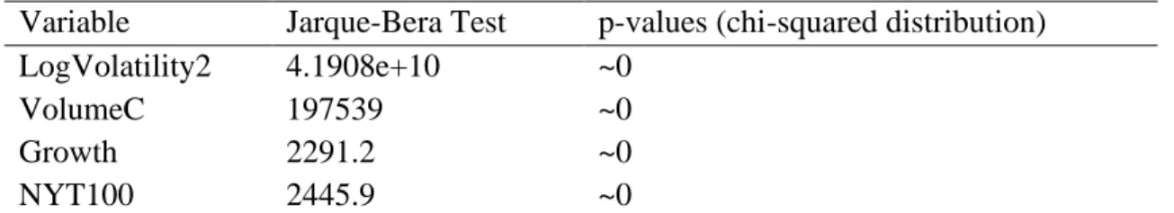
5.2.2. Bivariate correlations between variables ... 36
5.2.3. Stationarity in the Variables ... 37
6. Hypothesis Testing: Results ... 39
6.1. Testing the Normal Model ... 39
6.2. Analysis of the Residuals... 41
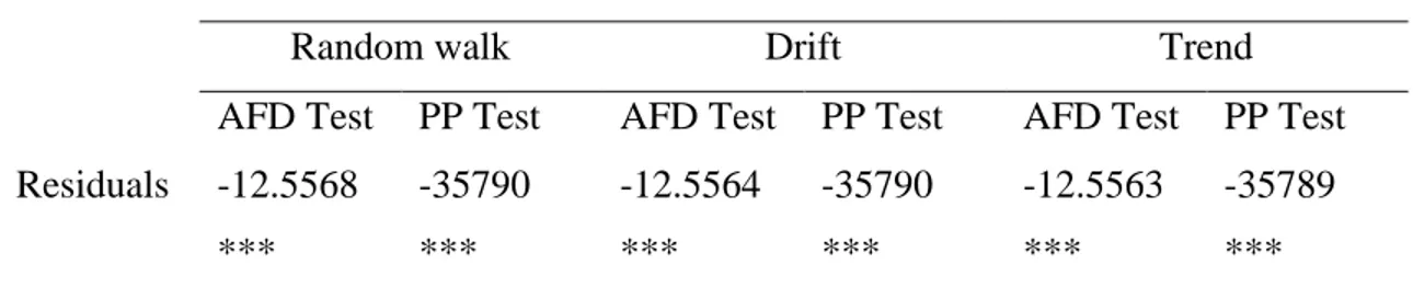
6.3. Stationarity of the Residuals ... 41
6.3.1. Checking Heteroscedasticity with a Breusch-Pagan Test. ... 42
6.3.2. Checking Autocorrelation... 42
6.4. Testing Other Models ... 44
6.4.1. Testing a Model with Added Variables ... 44
4
6.4.3. Findings from the Different Frame Times ... 48
7. Conclusions ... 50
7.1. Revisiting the Hypothesis, Results and Discussion ... 50
7.2. Conclusion & Suggestions for Further Research... 52
8. Bibliography ... 54 9. Annexes ... 57 9.1. Annex A ... 57 9.2. Annex B ... 58 9.3. Annex C ... 58 9.4. Annex D ... 59 9.5. Annex E ... 59 9.6. Annex F ... 60 9.7. Annex G ... 60
9.8. Annex H: Results Table ... 61
List of tables Table 1. Evolution of the US STT over time ... 16
Table 2. Evolution of the NY STT over time ... 17
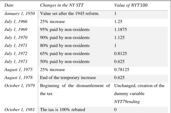
Table 3. Existence of the NY STT through time, value index 1 in 1950 ... 33
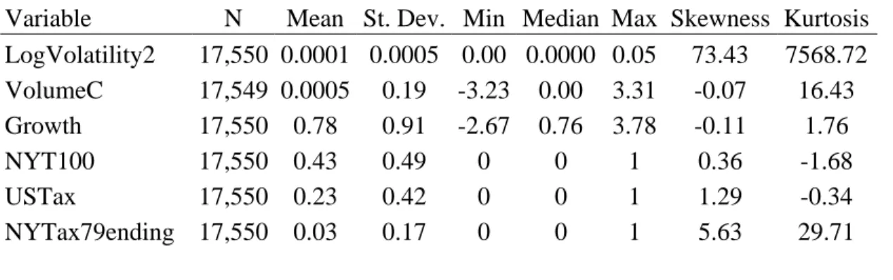
Table 4. Descriptive statistics of the variable of the model ... 35
Table 5. Jarque-Bera test-statistics and p-values for the variables ... 36
Table 6. ADF and PP Tests on the variables of the model ... 38
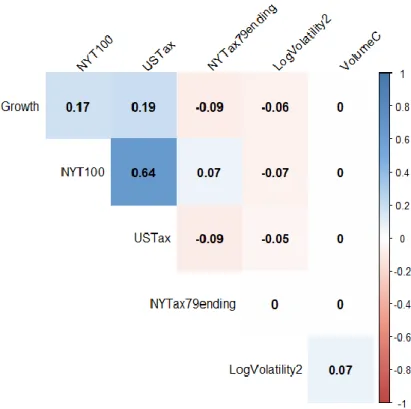
Table 7. OLS estimated parameters ... 40
Table 8. ADF and PP Tests on the residuals of the model ... 42
Table 9. Results of the Breusch-Pagan test on the residuals ... 42
Table 10. Results of the Breusch-Godfrey test on the residuals ... 43
Table 11. OLS estimated parameters with OLS and HAC Standard Errors ... 43
Table 12. Estimated coefficients for the model and the model with added variables with their OLS and HAC Standard Errors ... 45
Table 13. Estimated coefficients for the model and the period-models with HAC Standard Errors ... 49
Table 14. Other STTs in the world ... 58
Table 15. Jarque-Bera test-statistics and p-values for the residuals ... 60
Table 16. OLS estimated parameters with OLS, White and HAC Standard Errors ... 62
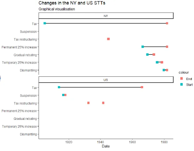
List of figures Figure 1. Changes in the NY and US STTs ... 18
Figure 2. Theorization of volatility: Breaking volatility into smaller factors ... 30
Figure 3. Correlations among the variables in the model ... 37
Figure 4. Estimated coefficients with their confidence intervals ... 40
Figure 5. Estimated coefficients with their confidence intervals, OLS and HAC SE ... 44
Figure 6.Estimated coefficients for the model and the model with added variables with their confidence intervals, OLS and HAC Standard Errors ... 46
Figure 7. The selected sub-periods ... 47
Figure 8. Estimated coefficients for the model and the period-models with their confidence intervals, OLS and HAC Standard Errors ... 50
5
List of Abbreviations
ADF Augmented Dickey Fuller
AIC Akaike Information Criterion
AMEX American Stock Exchange
BG Breusch-Godfrey
BLUE Best Linear Unbiased Estimator
BP Breusch-Pagan
BTT Bank Transaction Taxes
CI Confidence interval
CTT Currency Transaction Tax
Eq. Equation
FAT Financial Activities Tax
FTSE Financial Times Stock Exchange
FTT Financial Transaction Tax
GARCH Generalised Autoregressive Conditional Heteroscedasticity
GDP Gross Domestic Product
GLS Generalised Least Squares
HAC Heteroscedasticity- and Autocorrelation-Consistent
LSE London Stock Exchange
Min Minimum
Max Maximum
N Size
NASDAQ National Association of
Securities Dealers Automated Quotations
NY New York Stock Exchange
Market
NYSE New York Stock Exchange Market
OECD Organisation for Economic Co-operation and Development
OLS Ordinary Least Squares
OTC Over-the-counter
Pctl Percentile
PP Phillips–Perron
RGDP Real Gross Domestic Product
S&P 500 Standard & Poor's 500
SE Standard Errors
St. Dev. Standard Deviation
STT Security Transaction Tax
US United States
USD United States Dollars
6
1. Introduction
Global financial markets have evolved quickly during the last decades. Stock trade has grown quickly while the real economy has staggered in comparison: worldwide currency transactions are 70 times higher than the trade of goods and services, while European derivatives trading is nearly 100 times higher than Europe’s nominal GDP (Werner, 2003, p. 511; Schulmeister, Schratzenstaller, & Picek, 2008, p. 1). The US over-the-counter (OTC) derivative trade value in the first half of 2019, which accounts only for a portion of the total trades, was 640 USD trillion, compared to the world’s aggregated GDP at 80 USD trillion – meaning that OTC derivative trade in the US alone is eight times larger than the whole world’s GDP (Bank for International Settlements, 2019). Derivatives are one of the three main groups of financial instruments, altogether with debt and stocks.
Asset turnover has accelerated in speed, shown by the average time of holding securities going from 1.8 years in 1990 to 0.4 years in 2009 (Matheson, 2011, p. 19). Algorithm trading, known for malfunctioning and producing “cascading of correlated trades” that disrupted the market by generating herd behaviour and financial volatility, has skyrocketed from a 30% of the US equity trade in 2006 to representing 80% of it in 2016 (Matheson, 2011, p. 19-20; Alessandro & Alfredo, 2018). Volatility refers to the variation on asset prices in the financial market.
Despite this scenario, the markets have generally been deregulated by legislators, and the academic discourse is still unexplored, being mostly explored only immediately after the financial crisis of 2007-2008 (Schulmeister, Schratzenstaller, & Picek, 2008, p. 4). Data on the revealed characteristics of financial markets tends to be difficult to access, which makes it difficult to research on the topic.
1.1. Purpose
Measures against uncontrolled financial volatility have been attempted in several countries. Volatility is linked, if unchecked, to financial and economic crises, as it is explored at section 2.3. In the European Union, for example, the European Commission failed to reach a majority to pass a Financial Transaction Tax (FTT), which are taxes levied on financial market activity as explained in section 2.5 (German delegation, 2019, p. 2). In 2019, France and Germany once more showed public support for the measure and pushed together for the implementation of a European-level FTT, reopening the European debate (German
7 delegation, 2019, p. 2).
One of the reasons to support such tax is the current state of the financial world. In a world that faces an unregulated financial market, prices have turned more and more volatile and governments have lagged behind when public policy was needed.
One subgroup of FTTs that is gaining traction is Security Transaction Taxes (STT). While they are seen by economists and legislators as a way to reduce price volatility, they have been criticised by detractors in the same research field that claim that STTs increase volatility instead (Tobin, Prologue, 1996, p. xiii; McCulloch & Pacillo, 2011, p. 15). The published literature has focused on analysing these two opposite views in the advent and immediate aftermath of the implementation of an STT, and has rarely widened its scope to a bigger picture that includes the long-term. This tendency to focus on short-term data may be problematic, as the theorised effect of STTs on volatility is not only on the short-term but also on the long-term – meaning that long-term research could reveal if volatility happens to fall eventually instead of immediately after the introduction of an STT (Jones & Seguin, 1997, p. 728; Matheson, 2011, pp. 20-21; Schulmeister, Schratzenstaller, & Picek, 2008, pp. 7, 11, 34, 36).
This thesis contributes to the current debate by analysing the effect of STTs on volatility in the long-term, with the aim to provide input for the ongoing debate regarding STTs in the European Union.
1.2. Research Question
This research aims at covering the research gap on the long-term effect of STTs on volatility. The thesis focuses on two of the most well established and largest Western stock markets, the New York Stock Exchange (NYSE) and the National Association of Securities Dealers Automated Quotations (NASDAQ) financial markets, as reported by the Standard and Poor’s (S&P) 500 index. The State of New York allows the study of the long-term effect of STTs on volatility because it has a large amount of available data. The past effect of STTs in New York could set clear guidelines for future legislation on other markets, especially in the European Union. The researched period, 1950-2019, is a practical one, as it leverages all the available data from the S&P500 index.
This thesis answers the following question: To what extent did the New York State’s
8
markets, namely the NYSE and NASDAQ, between 1950 and 2019?
To answer this question, the effect of the two STTs that existed in New York during the studied period is analysed when controlling for other relevant effects such as trade volume and the performance of the real economy. This allows to quantitatively test a model suggested by theory where volatility is affected by the existence of STTs. The findings of the presented study are of interest to policy makers, as they show that STTs do not increase financial volatility in the long-term, while the NY STT decreases it. This paper also reveals that the relation between STTs and volatility must be studied in the long-term, since short-term studies are misleading because they may fail to capture the full extent of the STT’s impact.
1.3. Structure of the Thesis
This paper starts off by briefly explaining the functioning of financial markets and volatility to discuss the reasons behind STTs in the Background section. The Background section also outlines the history of STTs in the United States (US) and New York (NY). In the Literature Review the existent literature that analyses STTs in different countries is surveyed, focusing on the effects of STTs on trade volume in Sweden, the UK and other countries, and how this affects volatility in the respective country’s financial markets.
The Theory section explains the main approaches to understanding the relation between volatility and STTs. There, the hypothesis that STTs have a long-term effect on volatility, whether positive or negative, is set; and it is tested with a statistical model. The Methods and Source Material section is dedicated to explaining the model used in the thesis and the chosen control variables in more detail. The hypothesis is tested under the specified model on the long-term (1950-2019), under shorter periods of time (1950-1971, 1971-1993, 1950-1993, 1950-1980, and 1966-2019), and under an auxiliary model to check for the statistical robustness of the original model.
From there conclusions are drawn, which are that the NY STT had a statistically significant negative impact on volatility in the long-term while the US STT’s impact was not statistically significant. The results do not always hold when analysing this relationship under shorter periods of time, pointing out at the importance of executing long-term research when examining the relation between STTs and volatility.
1.4. Ontology and Epistemology
9 previous knowledge in the discipline. Therefore, a positivist epistemology is followed in which the relationship between STTs and financial volatility is researched through empirically testing theoretical expectations. Quantitative methods are used to process the large amount of data in the time-series used in the study. Regarding its ontology, this thesis assumes that the studied phenomena exist independently from each other to some degree, which frames it as an objectivist reasoning (Bryman, 2012, p. 27-28, 32, 36).
2. Background
2.1. What is the Financial Market?
A financial market is the place where financial transactions take place. Financial transactions are “any (contractual) transfer of financial assets” or “any payment of money (cash or transfer) between a buyer and a seller attached to the (contractual) transfer of a right with an economic value” (Commission Staff Working Paper, 2011c, p. 2). Financial assets include a wide set of concepts such as “equities, bonds, derivative contracts, structured products, repos or currencies” (Commission Staff Working Paper, 2011c, p. 2). In the case of corporate equity, it is understood as “stocks”, which usually pay a dividend to the corporation’s investors (Wright, 2012, p. 137).
There are a few things that limit the efficiency on financial markets: information is usually asymmetric, which means that all parties have access to different amounts and quality of information. Moreover, there are externalities, which means that what happens on the market affects and is affected by the outside world (McCulloch & Pacillo, 2011, p. 19). Not accounting for these market imperfections and relying on the idea that “markets know best” has been the circumstance to large waves of transactions that, when left unchecked, have damaged economies and generated crashes such as in the financial crisis of 2007-2008 (Schulmeister, 2010, pp. 16-19; Tobin, Prologue, 1996, p. xiii). Asset prices are not stable by default, as they tend to fluctuate upwards (bull markets) and downwards (bear markets) in the long-term, as well as up and down in the short-term (Schulmeister, Schratzenstaller, & Picek, 2008, p. 44). The difference between the long- and short-term is the period that is taken into account. Although there is no defined measure of time to distinguish between the two definitions, section 2.2 develops how they are described in this thesis.
10
2.2. Defining the short-term and the long-term
The focus of this thesis is to analyse long-term financial volatility compared to the more common short-term approach used in research, as explained in section 3. In section 3.1, a review on the existing literature reveals that its focal point is short-term financial volatility, although none of the consulted researchers provides clear descriptions when using a short and long-term scope.
Since the inception of the terms short and long-term by 19th century economist Alfred Marshall, many theorists have written about its boundaries. Soon after their creation, these terms have had a changing meaning depending on the field of study within the discipline of economics and depending on the theoretical basis of authors (Panico & Petri, 2008, pp. 190-191).
Mainstream economics describes the short-term as “a period of time in which at least one of the factors of production is fixed”, that is, where inputs to production do not vary. For long-term, on the other hand, there is no fixed input (Hoag & Hoag, 2006). This definition assumes a state of equilibrium for supply and demand, theoretically called long-term, and considers the deviations to such equilibrium to be the short-term.
Since this study lies within the field of economic history, a theoretical point of equilibrium is incompatible with the empirical analysis of data. As mentioned in section 3, the existing literature does not explicitly state the difference between short and long-term, classifying themselves as short or long-term based on the length of the period in which their observation is taken. Hence, instead of having a theoretically defined short and long-term, a practical one has emerged in the field of financial volatility.
As the aim of the paper is to focus on long-term volatility, the definition of long-term is constructed as a juxtaposition to the scope of the previous research, which is rarely done on periods longer than twenty years. Short-term, in this paper, is a period of time shorter than twenty years, while long-ren is an analysis of a longer span.
2.3. What Is Volatility?
Volatility is defined as the measure of the variation of asset prices in the financial market. Thus, if asset prices vary often and to a large extent in a given market, this market will be more volatile than one where asset prices remain fairly stable with a reduced amount of swings. The causes of high volatility are different in different narratives, as it will be seen
11 in sections 4.1 and 4.2, and it is either understood as depending on short-term speculative operations, on lacking liquidity, on excessive leverage, or on agent and institutional composition of markets (Matheson, 2011, p. 37; McCulloch & Pacillo, 2011, p. 25-26).
Higher volatility is generally considered to generate unstable markets and crashes, and the theoretical divergences on the topic focus on its origin rather than its effects. Markets where prices rise (decrease) more often in the short-term become bull (bear) markets, and stock prices tend to be “overshooting” and have “whipsaws”1. These random movements generate feedback loops that create persistent trends in the long-term based on short-term changes (Schulmeister, 2010, pp. 2-5; Schulmeister, Schratzenstaller, & Picek, 2008, p. 34-36, 44-45).
Since long-term volatility has negative effects on the real economy such as inflation/deflation and unemployment, Keynes and Tobin condemned short-term trading, which they considered to be its cause, for being a zero-sum game for the financial market that only generates volatility through speculation – leading them to propose STTs as a solution to it (Matheson, 2011, p. 20, 22).
2.4. What Are Transaction Costs?
Transaction costs are the expenses related to buying or selling assets, and they are not part of their perceived market price. They so far have been one reason why international prices were kept separated from each other, as financial transactions may not be profitable if they include a large transaction cost such as “broker commissions; dealer spreads; bank fees; legal fees; search-, selection-, and monitoring costs; and the opportunity cost of time devoted to investment-related activities” (Wright, 2012, p. 143, 164). Transaction costs still exist, even if they have plummeted due to the advances in information technology, as financial deregulation and the creation of new financial instruments.2 These changes do not only reduce transaction costs, but also allow faster trading in the financial market (Matheson, 2011, p. 19).
1 Overshooting refers to the tendency of financial markets to overreact to events with great changes in
prices, and whipsaws refers to sudden changes in the price trend of a stock – for example, from an increasing price to a fall or vice versa.
2 A financial instrument is any possible contract based on ownership or debt related to securities, and
they are the bulk of financial markets. Options and futures are amongst the most commonly dealt instruments, although instruments such as mortgage-backed securities have grown in size in the last years and even given name to a financial crisis in the Western World (U.S. Securities and Exchange Commission, 2010). An interesting report on recently created financial instruments can be found at Jakimowicz et al., 2017.
12 This reduction of transaction costs has increased speculation (to invest on risky assets with the goal to generate profit from price changes rather than investing to obtain returns or dividends) in all financial markets over the last three decades, leading to higher volatility and consequently more frequent financial crashes, which have had a negative impact on the real economy (Matheson, 2011, p. 30; McCulloch & Pacillo, 2011, pp. 28-32; Schulmeister, Schratzenstaller, & Picek, 2008, p. 4). Legislators have not enacted policies to counterbalance this phenomenon, lifting regulations and restrictions instead. To reverse this process, economist James Tobin proposed to tax financial transactions as a way to increase their costs. By doing so, volatility would be reduced – and so would its negative effects on the financial market. The next section gives an overview of the idea of taxing financial transactions (Schulmeister, Schratzenstaller, & Picek, 2008, p. 4).
2.5. Background on STTs
Financial Transaction Taxes (FTT) are a group of taxes on financial instruments including shares, bonds, and the trades in derivatives and excluding the payment of bills and regular bank transferences (Commission Staff Working Paper, 2011a, p. 30). The effect of an FTT to agents in the financial markets is increased transaction costs. The idea behind FTTs is using taxation to smoothen the functioning of the financial sector by making high-frequency trading less profitable, reducing speculation and thus reduce volatility (Commission Staff Working Paper, 2011a, p. 15).
FTTs are mainly comprised by two other subgroups, Currency Transaction Taxes (CTT) and Security Transaction Taxes (STT), as well as several smaller ones such as Bank Transaction Taxes (BTT) on deposits and withdrawals, Capital Levy Taxes on issuing assets and loans, Insurance Premium Taxes, Real Estate Transaction taxes on the value of land and structure, Financial Activities Taxes (FAT) on profit of financial institutions, and Value-Added Taxes (VAT) over assets (Commission Staff Working Paper, 2011a, p. 31; Matheson, 2011, p. 5-7). These, as well as CTTs, have been excluded from the scope of this thesis, which has the aim to broaden research regarding STTs and volatility after STTs regained public renown within policymakers in the last decade (Commission Staff Working Paper, 2011a, p. 5).
A CTT is a “securities transactions tax imposed specifically on foreign exchange transactions and possibly also their derivatives”, levied on the volume of currency trade
13 (Matheson, 2011, p. 5). First devised by British economist John Maynard Keynes in the 1930s, he saw it as a way to reduce financial bubbles without hindering investment on the real economy to make sure that finance was not driven by speculation (Matheson, 2011, p. 12). James Tobin, an American economist, popularized the idea and suggested a 1% global tax on transactions in these markets, popularising the tax to the degree to which “Tobin Tax” became an alternative name to CTTs (Matheson, 2011, p. 12). Tobin claimed that the tax would hurt speculators more than it hurts sophisticated traders, as they trade more frequently (Tobin, 1978, p. 155). Tobin’s approach is aligned with the bases of STTs, explained in the next section, once one changes the concept “currency” for “financial instrument”. (McCulloch & Pacillo, 2011, p. 15).
2.5.1. What are STTs?
An STT is a tax on the volume of transactions with “equity securities, debt securities and alike products (e.g. certificates, warrants, units in funds, structured notes etc.) and related derivative products including options, swaps, futures and forwards traded in exchanges and over-the-counter (OTC)”, the last one not being publicly traded and registered (Commission Staff Working Paper, 2011c, p. 2). The idea behind them is to shield an optimal product price interval making trading not profitable in this range of prices, ensuring that no trade is being done around the perceived price of assets to reduce short-term trading (Matheson, 2011, p. 13; Tobin, Prologue, 1996, p. xiii). The largest difference between STTs and CTTs is the market they are targeted to, as the former operates on financial markets while the latter does so on exchange markets.
STTs aim to decrease volatility by increasing transaction costs, which would reduce the profit of speculative trading and, in consequence, the amount of non-profitable trades (Matheson, 2011, p. 15; Song & Zhang, 2005, p. 1103). Since corporate bonds are less traded in frequency than stocks, the impact of STTs should not damage corporate borrowing – focussing its effects on fast trades that destabilise the market (Matheson, 2011, p. 15).
2.5.2. Designing an STT
When designing an STT, it is essential to consider who collects the tax, what is taxed, and who is taxed in order to avoid the negative consequences of badly designed of STTs3. If
3 For more information on what to consider, read McCulloch & Pacillo, 2011, p. 36; Commission Staff
14 an STT is badly designed, volatility will not be reduced as actors will shift from taxed instruments to untaxed ones (substitution) or to untaxed markets (migration). In this scenario, the negative effects of the STT may generate the financial and economic recessions they are trying to prevent, as stated with the 1984 Swedish example in section 3.1 (McCulloch & Pacillo, 2011, p. 11-12).
Regarding the tax collection, it is essential to avoid double transaction issues, and states should decide on each other’s jurisdiction on the financial market (Commission Staff Working Paper, 2011c, p. 17). Tobin suggested the tax being collected by each government independently and agreeing on a way to ensure international cooperation, as he foresaw that enacting an FTT in one single country could result in massive migrations of financial trade towards foreign markets (Tobin, 1978, p. 158; Tobin, 1996, p. xiv, xvii).
When deciding on the subject of taxation, it is important to include all instruments with high substitutability at similar rates to avoid a shift, as well as swap contracts and derivatives derived from the original instruments (McCulloch & Pacillo, 2011, p. 28, 31, 35). There also exists a debate in the literature on how to tax different assets according to their risk, transparency, and volatility to ensure the lightest impact on substitution and migration on the taxed financial market (McCulloch & Pacillo, 2011, p. 36).
When deciding on which actors are suitable to be taxed, legislators can usually choose from three options. A tax based on a residency principle means that nationals would be at a disadvantage in front of foreign investors, forcing locals out of the market (Commission Staff Working Paper, 2011c, p. 6). Taxing on the source principle means taxing the place of transaction and would reduce administrative costs while having a higher risk of relocation (Commission Staff Working Paper, 2011c, p. 8). Taxing on the domestic issuance principle means taxing all transactions related to domestic assets, which could result on a decrease of the amount of transactions in the country (Commission Staff Working Paper, 2011c, p. 8).
Apart from who to tax and what to tax, other details should be taken into account when designing an STT. For instance, even if only a single country could implement an STT, it is always preferable to standardize them internationally to discourage migration and avoid uncoordinated measures and avoid substitution and migration effects – increasing the efficiency of the tax to limit volatility (Commission Staff Working Paper, 2011a, p. 19; McCulloch & Pacillo, 2011, p. 42).
15 The number of countries with STTs has decreased sharply during the last decades, as many countries have severely cut and abolished them. The countries that have acted like this in the Organisation for Economic Co-operation and Development (OECD) include Austria, Belgium, Denmark, Germany, Ireland, the Netherlands, Spain, Sweden and the US (Schulmeister, Schratzenstaller, & Picek, 2008, p. 14). In Europe, STTs were prevented by EU legislation until 1985, and attempts to fully remove them were reborn in 2006 (Schulmeister, Schratzenstaller, & Picek, 2008, p. 15). However, some countries have recently created STTs, such as France and Italy (2012 and 2013) in their desire to promote the idea in the EU (Becchettia, Ferraria, & Trenta, 2014, p. 128). A table with some examples of STTs can be found in Annex A. Despite representing a challenge to legislators, the International Monetary Fund (IMF) has publicly stated that the global implementation of such tax would be feasible – even if discouraging it under the premise that it would not have an impact on volatility (IMF, 2010, p. 19; McCulloch & Pacillo, 2011, p. 41).
2.6. STTs in the US
STTs are not a new concept. Many have existed in the past, and they have been implemented all through the world as seen in Annex A. However, this thesis focuses on the United States, in New York, as it is one of the major centres of financial trade in the world and it was subjected to two different financial taxes: a national US STT and a local NY STT. Since the taxes on New York and the United States existed for extended periods of time and disappeared half a century ago, there is plenty of data of the financial markets before and after the taxes were implemented. At the same time, as one of the most important financial centres in the world, the NY stock market should be relatively free from migratory effects, as NY is considered a safe market by sophisticated investors even under financial crises (McCulloch & Pacillo, 2011, p. 11-12; Schulmeister, Schratzenstaller, & Picek, 2008, p. 19). Both taxes, national and local STTs, are presented in this section.
2.6.1. United States STT (1914-1966)
In 1914, war broke out in Europe. To offset the decreasing custom revenue, the American government under Woodrow Wilson implemented a nationwide tax on all security transactions on December 1, which was briefly suspended between September 1916 and December 1917. The tax was restructured in 1932 and was changed once again on September 20, 1941, both under Franklin D. Roosevelt’s presidencies. The tax remained unchanged until
16 January 1, 1966, when it was definitely abolished (Pomeranets & Weaver, 2018, p. 459). Its exact tax values are seen in Table 1.
2.6.2. New York STT (1905-1981)
The history of the State of New York with STTs began in 1905 with the creation of a tax on all stocks “traded, transferred, or delivered in New York” to reduce the state deficit. To a practical extent, and with some small modifications (some of which were quickly declared unconstitutional by the New York Supreme Court), the tax rate was 0.02% of the par value of the traded stocks. The tax was doubled during the Great Depression (Pomeranets & Weaver, 2018, p. 457).
Since taxing on par value means that companies could change the nominal value of their shares while the actual price would remain unchanged, the tax was changed to tax the trading price in 1933. The tax rates changed into a scaled system in 1945 as can be seen in Table 2, and remained unchanged until 1966 – when all the taxes were increased by 25%. After being lobbied by the NYSE, an amendment to the tax was passed in 1968 to prepare for an eventual reduction of the tax rate for non-residents by July 1973, at a time when 88% of the US investors in New York resided elsewhere. The tax saw another 25% surcharge between 1975 and 1978. The tax started to be dismantled in 1979 after the US Supreme Court ruled that the 1968 amendments were unconstitutional, which led to progressive rebates to residents and non-residents. On October 1, 1981, the tax received a 100% rebate for all traders, which is still in existence in 2021. The exact tax values can be found in Table 2.
Date Changes in the US STT
1914 $0.02 per 100 of par value.
September 1916 – December 1917 Temporary suspension of the tax.
June 21, 1932 $0.04 per $100 of par value.
If the stock value was above $20, $0.05 per $100 of par value.
September 20 1941 $0.05 per $100 of par value.
If the stock value was above $20, $0.06 per $100 of par value.
January 1, 1966 Tax repealed.
17 Figure 1 graphically depicts the changes in the NY and US STTs (Pomeranets & Weaver, 2018, p. 458).
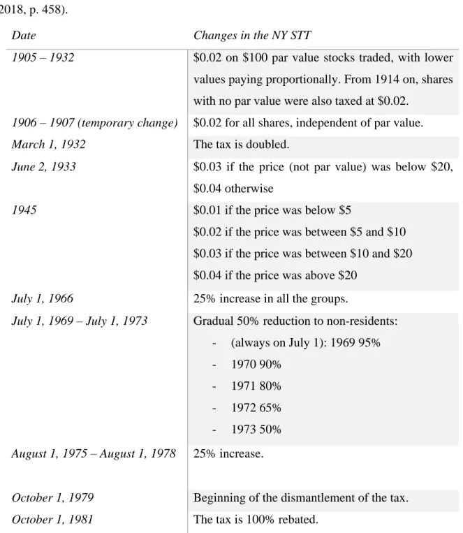
Date Changes in the NY STT
1905 – 1932 $0.02 on $100 par value stocks traded, with lower
values paying proportionally. From 1914 on, shares with no par value were also taxed at $0.02.
1906 – 1907 (temporary change) $0.02 for all shares, independent of par value.
March 1, 1932 The tax is doubled.
June 2, 1933 $0.03 if the price (not par value) was below $20, $0.04 otherwise
1945 $0.01 if the price was below $5
$0.02 if the price was between $5 and $10 $0.03 if the price was between $10 and $20 $0.04 if the price was above $20
July 1, 1966 25% increase in all the groups.
July 1, 1969 – July 1, 1973 Gradual 50% reduction to non-residents: - (always on July 1): 1969 95% - 1970 90%
- 1971 80% - 1972 65% - 1973 50%
August 1, 1975 – August 1, 1978 25% increase.
October 1, 1979 Beginning of the dismantlement of the tax.
October 1, 1981 The tax is 100% rebated.
Table 2. Evolution of the NY STT over time. Sources: Pomeranets & Weaver, 2018, p. 459; New York State, 2020.
18
3. Literature Review: Empirical Examples
Previous studies on STTs share two common features: Firstly, preceding literature on the connection between STTs and volatility does not have uniform definitions, not even for basic concepts. For example, volatility is computed differently in several of the reviewed papers4. Secondly, most studies were conducted for short periods of time because data were missing. Consequently, the literature falls short to analyse the long-term effects of STTs (McCulloch & Pacillo, 2011, p. 28). This section reviews the results of previous studies on volatility and STTs keeping these limitations in mind, grouped by the countries they examine.
4 For some examples, Becchetti et al., 2014 (130): 𝑉𝑜𝑙𝑎𝑡𝑖𝑙𝑖𝑡𝑦
𝑝2=
ln2(𝐷𝑎𝑖𝑙𝑦 𝐻𝑖𝑔ℎ𝑖𝑡⁄𝐷𝑎𝑖𝑙𝑦 𝐿𝑜𝑤𝑖𝑡)
4∗ln 2
Jones, 1997(732) assumes constant volatility in each year and estimates it as 𝑉𝑜𝑙𝑎𝑡𝑖𝑙𝑖𝑡𝑦 = 𝑆𝐷(𝐷𝑎𝑖𝑙𝑦 𝑟𝑒𝑡𝑢𝑟𝑛𝑠)𝑡− 𝑆𝐷(𝐷𝑎𝑖𝑙𝑦 𝑟𝑒𝑡𝑢𝑟𝑛𝑠)𝑡−1. Both refer to the year before and the year after the tax.
Song & Zhang, 2005 (1107-1110) calculate a formula based on individual expectations, which is out of the scope of this paper.
Hanke, 2010, explains volatility as a random walk without drift and bases it solely on the fundamental value of the trades in his lab-experiment.
19 Many of the articles on the field analyse countries within the European Union, as the data is widely accessible and has been the centre of a wider debate in EU politics after the financial crisis of 2007-2008. The US and the rest of the world have not been so deeply researched regarding the connection between STTs and volatility despite the decent amount of data available. The exception to this lack of research is regarding the relationship between the volume of trades and volatility – a field that has been widely explored in order to draw conclusions about the relationship between STTs and volatility. The reason behind might be that public discourse on the issue was lacking.
3.1. The Effect of an STT on Volatility
3.1.1. Indirect effects of STTs on Volatility: Effects of Volume on Volatility The findings on the impact of STTs on volatility are the subject of many studies. These studies reveal that research has been focused on two directions: one is measuring the impact of STTs on price volatility directly, and the other is measuring the impact of the volume of trades in volatility. The latter indirectly captures the effects of STTs, as these reduce volume according to the reviewed literature. This section explores the indirect effects of STTs on financial volatility through changes in the volume of trades, and section 3.1.2 reviews the direct effects of these taxes on volatility.
The findings of two major meta-studies, performed by Matheson (2011) and by Schulmeister, Schratzenstaller, and Picek (2008) report an important relationship between STTs and volume of transactions. Their findings estimate that the elasticity of the volume of transactions with respect of financial transaction costs oscillates between -0.25 to -1.7, meaning that a 1% increase on costs results in a 0.25% to 1.7% reduction of turnover – with the higher numbers theorised to be happening in the long-term (Matheson, 2011, p. 15, 18; Schulmeister, Schratzenstaller, & Picek, 2008, p. 19). None of the analysed studies contradicts this relationship.
Several studies researched the relationship between volume and volatility in the US. Bessembinder and Seguin (1993) analysed diverse assets in eight US financial markets between 1982 and 1990 and concluded that volume shocks have a positive impact on volatility – an especially strong relationship when it comes to increases in trades (Bessembinder & Seguin, 1993, pp. 21, 25, 37). The results are similar in French and Roll (1986), who concluded that the volume of trades is a main driver of volatility at the NYSE
20 and the American Stock Exchange (AMEX) between 1963 and 1982 (French & Roll, 1986, pp. 7-23). This relationship has been analysed under the scope of the very short-term in Huang, Cai, and Wang’s (2002) study. By using 10-minute intervals in the US Treasury notes trades in 1998, the authors concluded that there is a strong positive relationship between the trade frequency and price volatility in that market (Huang, Cai, & Wang, 2002, pp. 277, 293). This is the same conclusion reached by Sarwar (2003) in the exchange market, who uses several GARCH models to conclude that a strong positive relationship exists between volume of currency transactions and volatility within the British Pound between 1993 and 1995 (Sarwar, 2003, pp. 681, 685). With an innovative focus on the NASDAQ market between 1986 and 1991 Jones, Kaul, and Lipson (1994) determined that, while this positive relationship exists, more research on the topic must be carried out – as it may not be the volume of trade but just the amount of transaction the factor that generates volatility (Jones, Kaul, & Lipson, 1994, pp. 634, 645).
Overall, the literature on indirect effects agrees that there is a strong positive relationship between volume and volatility. Existing research indicates that increased (decreased) turnover results in higher (lower) levels of volatility. Previous research goes as far as to pin turnover as the causal mechanism and volatility as the outcome (Al-Jafari & Tliti, 2013, p. 47; Bessembinder & Seguin, 1993).
3.1.2. Direct Effects of STTs on Volatility
When it comes to the direct effects of STTs on volatility, there is less literature available referred to the US. The results related to countries that have been analysed more than once tend to be contradictory, resulting in mixed results even for the same financial markets.
Several papers have been published regarding markets in European countries. The Swedish and British STTs are the two best known examples of STTs in practise, both for different merits, and are the most studied ones. In the Swedish case, a tax was raised between 1984 and 1991, taxing buyers and sellers on Swedish stock exchange markets a 0.5% of the derivative price each (1% each from 1986 on). The tax, however, only applied to Swedish brokers and created unpredicted effects, notably the migration of traders to the London Stock Exchange (LSE), where a lower tax was enforced on all agents. The Stockholm Stock Exchange was then filled with foreign traders who were not subjected to the tax, most of
21 which acted as noise traders (Schulmeister, Schratzenstaller, & Picek, 2008, p. 21-24). The tax revenue accounted only for 3% of what legislators expected, and price volatility was not affected (Commission Staff Working Paper, 2011d, p. 8; Umlauf, 1993, p. 227). The Swedish STT was abolished in 1991 as a result of the failure of the experiment – standing in history as an example of bad tax design.
Umlauf’s Transaction taxes and the behaviour of the Swedish Stock Market (1993) has been highly influential within the field, as its findings are often reported as being incontestable evidence that STTs do not only not reduce volatility – but actually increase it (Jones & Seguin, 1997). Umlauf studies the Swedish stock market between 1980 and 1987 with short-term models that analyse stock volatility, and his final conclusions do not settle the debate: while he realises that volatility increases during some of the periods where the STT was in place, he also notices that his methods are imprecise because “theoretical foundations are lacking” and that his conclusions should not be generalised (Umlauf, 1993, pp. 235, 240). While his findings on the Swedish market are still very relevant, he remarks that “[t]he time horizon examined may be too short”, calling for further long-term research (Umlauf, 1993, p. 235).
Further research on Sweden exists, albeit related to the short-term and a different period. Nordén’s (2009) analysis of different periods between 2005 and 2007 on the OMX30 market in Stockholm concludes that a 22% reduction in the exchange fee on trades resulted on an increased 27% volatility, although the used data is centred around very short spans of time (Nordén, 2009, pp. 9, 11, 23, 30).
The Swedish experience proved that STTs may have a strong negative impact on the financial markets and the real economy, increasing volatility during the taxed periods. The Swedish STT, nonetheless, is only one of the several STTs that have existed – and still exist – in Europe. Contrasting the Swedish experience, the United Kingdom has shown less damaging results.
Dating from the 17th century, the British Stamp Duty Tax has been applied to several products such as stamps, newspapers, insurance policies, or precious metals (Archives, 2020). The current tax has been expanded and includes the Stamp Duty Reserve Tax (SDRT), resulting on a 0.5% tax on purchase price (on issuers if it is the primary market) of securities and document-free agreements (Schulmeister, Schratzenstaller, & Picek, 2008, p. 24).
22 Instead of taxing domestic asset transactions as the Swedish tax did, the British one focuses on transfers of assets owned by domestic companies. A drawback to the SDRT is the existence of legal ways to avoid the payment of the tax, as investors may issue “depository receipts” in other markets and trade in such untaxed instruments. As these actors still trade in British markets, migratory effects are prevented (Schulmeister, Schratzenstaller, & Picek, 2008, p. 25). The design of this STT has broadly been considered superior to the Swedish one as the revenue of the tax represented in 2019 a 0.5% of national budget without any negative effects on the market itself (Commission Staff Working Paper, 2011d, p. 4-7; HM Revenue & Customs, 2019, p. 2; Schulmeister, Schratzenstaller, & Picek, 2008, p. 26).
The findings on the British STT are however mixed as well. Saporta and Kan (1997) use a GARCH analysis on monthly data of the London Stock Exchange (LSE) between 1955 and 1995, with weekly and daily data for shorter periods of time, and conclude that there is no empirical evidence in their study that the British STT affects volatility (Saporta & Kan, 1997, pp. 30, 40). Green, Maggioni, and Murinde (2000) perform an extensive study on volatility on the LSE between 1870 and 1986, creating several indexes with monthly data not generally available to the public (Green, Maggioni, & Murinde, 2000, pp. 582-583). The data, when examined in the short-term, reveals that increased transaction costs result in increased volatility, although the longevity of their study allows them to discover that the long-term impact of increased transaction costs may differ from the short-term ones by having either no impact or a reduced volatility, opening the door to long-term analysis in the topic (Green, Maggioni, & Murinde, 2000, p. 595).
STTs in other countries have been researched to a lesser extent. The main reason behind these taxes has been extracting revenue from untaxed markets, and their impact on volatility is not often explored. Research on the French STT, which was performed when it was only applied to stocks trading above 500 French francs, has been performed by Hau (2006). Hau studies different assets with prices around these F500 in the Paris Bourse between 1995 and 1998, analysing their volatility when their price is above F500 (resulting in a taxed asset) and below F500 (resulting in an untaxed asset). His conclusion is that STTs increase volatility as a consequence of increased transaction costs (Hau, 2006, pp. 872,873, 888)
23 limited number. Jones and Seguin studied the NYSE, AMEX and NASDAQ between 1974 and 1976 analysing differently priced assets to conclude that reduced transaction costs after abolishing the NY STT resulted in lower volatility in such markets (Jones & Seguin, 1997, pp. 729, 731, 736). Their results are consistent with Wang and Yau (2000), who examine different financial contracts and their transaction costs in the NYSE and NASDAQ between 1990 and 1994 to reach the conclusion that financial contracts and “the imposition of a transaction tax” reduce the volume of trades, reducing market liquidity and, finally, increasing volatility (Wang & Yau, 2000, pp. 944, 953-954, 966).
The impact of STTs has been measured on Asian financial markets too, with mixed results as well. Chou and Wang (2006) analyse the period between 1999 and 2001 to measure the Taiwanese STT tax cut (from 0.5% to 0.25%) to conclude that the Taiwanese stock market’s volume increased after the change – but volatility remained steady (Chou & Wang, 2006, pp. 1195-1196, 1214). These results match with those of Hu (1998), who studied 14 tax changes in Hong Kong, Japan, Korea and Taiwan between 1975 and 1994 to conclude that there was no change in volatility – although he did not find a change in volume either. Hu’s research in several countries allows him to claim that the reason why volatility did not change in these markets is that there does not seem to be a migration effect between the financial markets of these countries (Hu, 1998, pp. 362-363).
Baltagi, Li and Li (2006) reach different conclusions in their study of Chinese stock markets with modified GARCH models. Their study, which spans for a year between 1996 and 1997, measures the increase of the Chinese STT from 0.3% to 0.5% on May 1997, resulting in a 33% reduction on turnover and a significant increase in volatility, as well as slowing down the market and not allowing price shocks to be assimilated (Baltagi, Li, & Li, 2006, pp. 393, 396, 400, 406). Another global meta-study, by Roll (1989), on 23 different national markets in different periods of time calculated a negative impact of STTs on volatility, but only to a non-significant level (Roll, 1989, pp. 236, 241).
With the ongoing European debate on STTs spanning for some years, a global meta-analysis on the effects of STTs was published by the European Commission in 2011. In the study, the authors pointed out the arguable focus on the short-term effects on volatility, as instead of the timespan being a decision made upon the needs of the studies it is often only motivated by a lack of data (Commission Staff Working Paper, 2011e, p. 7). Their results
24 indicate three general conclusions, one of them focusing on the impact of STTs on volatility: “The empirical finding mostly points to either no effect on price volatility or an increase in it due to a decreased number of transactions” (Commission Staff Working Paper, 2011e, p. 8).
There are several other STTs within countries of the EU that lack analysis. The tax on stock exchange transactions in Belgium (introduced in 2016) is levied on all trades with financial instruments agreed or executed in Belgium ignoring nationality and primary markets, taxing between 0.07% and 0.5% depending on the asset. Finland (introduced in 1997) taxes all transactions with at least one Finnish agent at a 1.6% of the share price. In the same way, Switzerland applies a tax on the same basis at a 0.15% for domestic assets, and 0.3% for foreign ones – although there are exceptions for some securities and bonds (Commission Staff Working Paper, 2011d, p. 2-3, 9-10).
Greece (introduced in 1998, with the current one set in 2011) collects its 0.2% STT on compound products, OTC and “the sale of foreign listed shares by Greek tax payers [sic]” (AthexGroup, 2020; Commission Staff Working Paper, 2011d, p. 4). In Poland (introduced in 2000), the Civil Law Activities Tax (CLAT) charges derivatives and securities with rights based in Poland with a 1% tax on buyers (BNY Mellon, 2020, p. 10; Commission Staff Working Paper, 2011d, p. 4). There is little to no research on these cases, mostly due to the taxes being recently implemented.
The effect of the relationship between transaction costs and volatility in the literature is ambiguous and not always visible, as changes in transaction costs and volume do not indicate that volatility is altered in the same way each time. The analyses, focused on the short-term, report inconsistent changes in volatility – which either increases, decreases, or remains unchanged after the introduction or disappearance of an STT (Commission Staff Working Paper, 2011e, p. 7-8; Hanke, Huber, Kirchler, & Sutter, 2010, p. 59; Song & Zhang, 2005, p. 1119).
Notwithstanding the reviewed literature’s conclusions being, at best, mixed and contradictory, an abridged conclusion can be summarised from the consulted papers. This conclusion is that there is an important gap in the existing literature, as articles set their focus on the short-term, analysing the effect of taxes on the immediacies of their implementation. Out of the examined articles, most of them focus on periods of time shorter than five years –
25 with only one paper taking an approach that includes a span of time longer than a century. There is no follow-up study of the papers that request long-term research on the taxes they have analysed, resulting in a recognised – but ignored – gap in the research on STTs and volatility. In fact, none of the papers refers to a definition of short and long-term, even when using the concepts in their analysis: the long-term is usually defined by the length of the period of time in which they observe the data itself.
4. Theory
4.1. Approaches to the Financial Markets and Security Prices
A research question was formulated in the introduction of this thesis regarding the impact of STTs on financial volatility. In order to determine the extent to which STTs impact volatility on the NY financial markets, the theoretical expectations for the STTs’ impact on volatility in general need to be clarified. The ongoing theoretical debate on STTs and volatility of asset prices is divided: one side argues that STTs reduce volatility by reducing the number of trades, while the other side says that STTs may instead increase volatility by making the assessment of the true value of an asset harder. Each of these perspectives is rooted on different assumptions regarding the operation of the market: the rational expectations narrative, reflexive narratives, and game theoretical approaches.
The narratives differ in their assumptions on how changes in supply and demand of shares are reflected in the stock market prices. The rational expectations narrative assumes actors to be intelligent and to make the best predictions with the available information (Phoa, Focardi, & Fabozz, 2007, p. 370-371). This perspective views changes in stock prices as a consequence of changes in the supply and demand of that stock. Hence, these changes in the supply and demand change the expectations of the traders, adjusting their perceived price on the asset and buying and selling it until the new market value reaches the new perceived value. This narrative considers non-extreme volatility to be a subproduct of this process of price adjustment and does not consider it to be a negative phenomenon if the market is flexible and capable of finding such equilibrium points, seeing STTs as an obstacle to the normal functioning of the process by impeding market actors from adjusting the prices correctly (Wright, 2012, p. 133).
26 market overreacts to price changes in assets as agents lose confidence in them and trigger bigger snowball effects in prices. Prices then become unstable, generating volatility (Phoa, Focardi, & Fabozz, 2007, p. 372).
The last main narrative is a collection of theories called game theoretical approaches. These theories defend that agents maximize utility inside of two different groups: commercial traders – also called sophisticated investors – and financial speculators – also called noise traders (McCulloch & Pacillo, 2011, p. 26). Following this logic, sophisticated investors act as intelligent actors that use their available information and trade following fundamental values of assets to try to locate sensible prices for assets (“price discovery”) and facilitate investment like predicted by the rational expectations narrative (Song & Zhang, 2005, p. 1107, 1111). On the other hand, noise traders affect the whole market in a negative way, overreacting to market changes, and creating shocks for every actor while getting a profit for themselves. Noise traders thus prevent price discovery as explained by the reflexive narrative (Matheson, 2011, p. 22; McCulloch & Pacillo, 2011, p. 20). Noise traders, by attempting to obtain short-term profit exploiting the market, are the source to sudden changes in prices and volatility generation.
Hence, volatility can either be the outcome of changing information according to the rational expectations narrative, or of investors who overreact to price changes according to the reflexive narrative and game theoretical approaches. The different narratives offer different understandings on how volatility is caused and consequently on how an STT impacts it. The next section is therefore aimed to discuss different theoretical perspectives on the impact of STTs and their respective in favour or against arguments for such a tax.
4.2. The Theory Behind Volatility
Theory on STTs is crafted around the public debate on the advantages and disadvantages of such a tax. Since this theory is (mostly) deducted from research, it is kept within the limitations of the current literature. Furthermore, theories are focused on short-term analyses, as long-short-term volatility studies are usually scarce due to the lack of data (Schulmeister, Schratzenstaller, & Picek, 2008, p. 11). Consequently, the paragraphs in section 4.2.1 and 4.2.2 mostly refer to the short-term. This allows this thesis to compare the short-term predictions with the results of the long-term analysis, and see how much of the established theory is sound in any period length.
27 On the basis of the different narratives and the understanding of the mechanisms of the financial market, two opposed views on how STTs impact volatility appear: according to the rational expectations narratives STTs may increase volatility as increased transaction costs make it harder for agents to adjust the prices of assets to their expectations. On the other hand, according to the reflexive narratives and the game theoretical approaches STTs may reduce volatility, as those noise traders may see their profit decrease and abandon their strategy. Hence, different arguments in favour and against STTs have been developed.
4.2.1. Arguments in Favour of STTs
Arguments that support the implementation of an STT mainly come from both the reflexive and game theoretical narratives. As Tobin explains with simple terms, “a 0.2% tax on a round trip […] costs 48% a year if transacted every business day, 10% if every week, 2.4% if every month” (Tobin, Prologue, 1996, p. xi). Thus, an STT should reduce the amount of noise traders operating on the market, and hence prevent speculation in trading (Becchettia, Ferraria, & Trenta, 2014, p. 128).
The tax would slow down trading and reduce liquidity, that is, the possibility to turn an asset into money for sellers. This would help stabilising financial markets in time of financial bonanza, ensuring that noise traders would have a more difficult time at making large benefits through speculation (Jones & Seguin, 1997, p. 728; Schulmeister, Schratzenstaller, & Picek, 2008, p. 7). The increased transaction costs would reduce speculative automated trading as well, as those fast trades benefiting from small changes on the price of a share would not result as profitable anymore (Commission Staff Working Paper, 2011a, p. 36).
As one can see, these positions are founded on the reflexive narrative and game theoretical approaches. Noise traders, the main cause of volatility, can be slowed down by decreasing the appeal of their speculative trades via an STT, resulting in a more stable market. In summary, STTs are thus the cause of a decrease on volatility.
4.2.2. Arguments against STTs
On the other hand of the debate, the theory based on the rational expectations narrative diverges with the conclusions reached by the defenders of STTs. From the point of view of that narrative, STTs reduce the number of asset trades, resulting in a slower price discovery for investors (or sophisticated investors if using the game theoretical approaches’
28 terms) and consequently in an increase of volatility (Matheson, 2011, p. 15; Werner, 2003, p. 511-512). The theorised increase on volatility is based on a simple hypothetical rule: the more transactions a market has, the more efficient it is (Matheson, 2011, p. 12, 14; Schulmeister, Schratzenstaller, & Picek, 2008, p. 7-8).
The theory also emphasises the impact that STTs have on the market itself by encouraging migratory effects towards other markets such as London in the previously discussed Swedish case in section 3.1.2, generating negative effects on the real economy while increasing volatility by decreasing the efficiency of financial markets by mispricing assets (Becchettia, Ferraria, & Trenta, 2014, p. 128; Commission Staff Working Paper, 2011a, p. 38, 50, 52; Hanke, Huber, Kirchler, & Sutter, 2010, p. 59; Jones & Seguin, 1997, p. 729). As a summary, the rational expectations narrative states that, instead of reducing noise traders, increased transaction costs cause slower price discovery for sophisticated investors which, at the same time, become a source of higher volatility.
It must be noted that a large proportion of the articles against STTs base their reasoning on Umlauf, 1993, a paper with strong positions on STTs after analysing the catastrophic effect of the Swedish STT, as a main reference for their study. Out of the reviewed articles on the topic, 15 out of 21 based part of their theory or conclusions on him, hinting at some degree of overrepresentation of his findings over those of other researchers.
4.3. Hypothesis
The aim of this thesis is to be able to fill the gaps on the long-term effects of the taxes on volatility, broadening the scope of previous research. The lack of long-term research on the relationship between STTs and volatility presents an utmost setback, setting the current standard for research on the short-term. Thus, short-term analyses are overrepresented on the debate on taxation of financial markets in the long-term, while they also present inconsistent results. This thesis introduces a different scope to the relationship which helps understand the impact of STTs in the long-term.
Three possible outcomes regarding volatility in the long-term may arise. Outcome A is that, in the long-term, STTs reduce volatility; Outcome B is that they increase it; and Outcome C is that they do not affect it. The following hypothesis aimed at setting a first brick to settle the speculation by analysing if STTs have any effect, positive or negative, on volatility in the long-term.
29 Hypothesis: STTs have a long-term effect on volatility in the financial markets where they are applied.
5. Methods and Source Material
5.1. Modelling Volatility5.1.1. Quantitative Methods: The OLS Model
To answer the research question on the long-term effects of STTs on volatility, a quantitative methodology is used to carry out a data analysis. Ideally, the period in question would cover the years from the implementation of the NY and US STTs – 1905 and 1914 respectively – until today in order to grasp the longest possible period of time. It is, however, not possible to access data on volume before 1950 and thus the first 45 and 36 years of the NY and US STTs cannot be covered in this study. The datapoints of the resulting period of 69 years are given in a time series format. To estimate the impact of the independent variables US STT and NY STT on volatility, the dependent variable, an Ordinary Least Squares (OLS) model is used, the fundamental statistical method for estimating linear regression models such as the one presented in this thesis. By estimating an OLS model inferences can be drawn about the actual impact of STTs on volatility in the NY financial market in the long-term (Gujarati, 2008, p. 107).
The OLS model is a multivariant regression, analysing the period from 1950 to 2019 with the variables that are relevant to understand volatility (the dependent variable), namely the volume of trade, an indicator for the real economy performance, and the taxes and the days of the week – all explained at section 5.1.3. Out of these variables, the variables for the STTs are the target independent variables, while the other ones are used as control variables to avoid spurious effects. In a second step, the model is broken into shorter sub-periods of time of 20 or more years each to check for the robustness of the results and to test the possible discrepancy in outcome between the analysis of models with shorter (although still long-term) models and the analysis of their holistic study.
5.1.2. The Theorization of Volatility
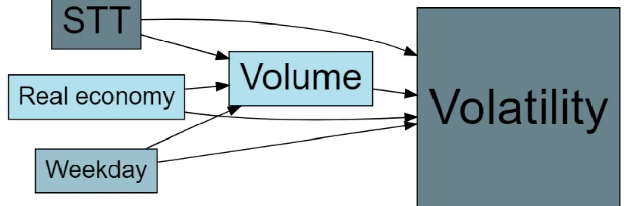
To analyse the impact of STTs on volatility a model is formulated based on the theory. Since the changes on volatility cannot be only attributed to the existence of STTs, the model includes several control variables, which are variables that have an impact on volatility as
30 well and that, if not accounted for, could bias the specifications (Gujarati, 2008, p. 422). Based on previous studies that determine that changes in the real economy also fuel (or hinder) the financial market and consequently influence volatility, those are included in the model to, once more, avoid a misspecification the model (Rodrigues da Silva, Tabak, Oliveira Cajueiro, & Fazio, 2018, p. 6-8; Borio, Drehmann, & Xia, 2018, p. 62-64). One last factor is included to control seasonality, namely the day of the week of the observation, which follow a seasonal pattern (Becchettia, Ferraria, & Trenta, 2014, p. 136; Berument & Kiymaz , 2001, pp. 190-191; Flannery & Protopadakis, 1988).
Following the literature, volatility itself depends on many factors, most prominently the performance of the real economy, the trade volume of securities, the day of the week, and the presence of an STT. The diagram below represents how these factors influence each other, built on the consulted literature in section 3 and the theory on STTs and volatility from section 4. STTs influence volatility in two ways, directly and indirectly by limiting the volume of trade. The impact of the other relevant variables, namely volume, the performance of the real economy, and the day of the week, are presented in section 5.1.3,Formulating a Model and are displayed below in Figure 2.
In this model, volatility takes the place of the dependent variable. The independent variables are the STTs that were in place in the NY market in the observed period: the New York STT and the United States STT. To answer to the research question in order to accept or reject the hypothesis the impact of both STTs and their significance are analysed. The measures for these variables are described in the following section.
31 5.1.3. Choosing Variables for the Model
To analyse price volatility, the dependent variable of the model, the daily closing value of the analysed financial market is used as measured by the S&P500 index. This index calculates the performance of the stocks of the 500 largest companies in the US, which must be registered either in the NYSE or the NASDAQ. The S&P500 is the most commonly used index of the US stock market (S&P Dow Jones Indices, 2020, p. 10; S&P Global, 2020) 5.
To compute volatility, two transformations are applied to the original index. Firstly, S&P500 data are transformed into their percentual change of prices between days, calculated as
𝐿𝑜𝑔𝑉𝑜𝑙𝑎𝑡𝑖𝑙𝑖𝑡𝑦𝑡= 𝐿𝑛 (
𝑃𝑡
𝑃𝑡−1
) Eq. 1
where 𝑃𝑡 is the closing value of the S&P500 index for day 𝑡 (Gujarati, 2008, p. 857; Cowpertwait & Metcalfe, 2009; Wang & Yau, 2000, p. 954).
Secondly, the data must be transformed to avoid having negative volatility (prices can vary more or less, but they can never vary less than zero) (Pomeranets & Weaver, 2018, p. 464). To do so the results are squared as 𝐿𝑜𝑔𝑉𝑜𝑙𝑎𝑡𝑖𝑙𝑖𝑡𝑦2𝑡= 𝐿𝑜𝑔𝑉𝑜𝑙𝑎𝑡𝑖𝑙𝑖𝑡𝑦𝑡2.
The data used to measure volatility, as well as volume (which is explained hereunder), are taken from Yahoo Finance (Yahoo!, 2020)67. The chosen timespan for the analysis has been influenced by the availability of the data, as the values for volume of trades were reported consistently only after January 1, 1950. Therefore, this marks the beginning of the analysed period – while its ending has been fixed at the arbitrary October 1, 2019, as it was the last complete data at the point of collection.
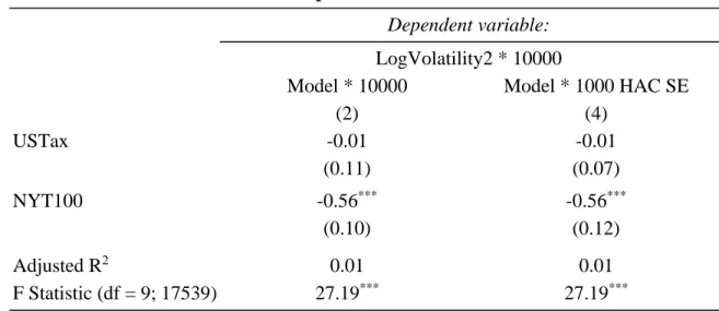
A dummy variable has been created under the name 𝑈𝑆𝑇𝑎𝑥 to indicate the existence of a national STT. In this case, 𝑈𝑆𝑇𝑎𝑥 = 1 indicates there is a tax present, while 𝑈𝑆𝑇𝑎𝑥 = 0 indicates there is not. This tax does not vary with years, and hence a dummy variable is the
5 More information on the eligibility criteria, the construction of the index, the calculations, the
maintenance and the data of the S&P500 can be found at S&P Dow Jones Indices, 2020.
6 All the data provided by Yahoo is taken from the Interactive Data Corporation (ICE) Data Services,
one of the main providers of financial data in the United States, as ICE does not provide it directly to individuals (Yahoo!, 2020).
7 Another reason to favour the S&P500 index over competitors is its public availability, as most of
other databases – not only for other countries, but for the United states too – presented many missing observations in their data. For example, the data published by the Financial Times Stock Exchange (FTSE) in diverse cities presented many missing observations, especially in regards to volume, as the data is not available to the wider audience and is shielded by their providers.