2017; 3(1): 11-27
Published by the Scandinavian Society for Person-Oriented Research Freely available at http://www.person-research.org
DOI: 10.17505/jpor.2017.02
11
Direction of effects in categorical variables:
Looking inside the table
Alexander von Eye
1and Wolfgang Wiedermann
21
Michigan State University
2
University of Missouri
Email address:
voneye@msu.edu
To cite this article:
von Eye, A., & Wiedermann, W. (2017). Direction of effects in categorical variables: Looking inside the table. Journal for Person-Oriented
Research, 3(1), 11-27. DOI: 10.17505/jpor.2017.02
Abstract: In the variable-oriented domain, direction of dependence analysis of metric variables is defined in terms of
changes that the independent (or causal) variable has on the univariate distribution of the dependent variable. In this article, we take a person-oriented perspective and extend this approach in two aspects, for categorical variables. First, instead of looking at univariate frequency distributions, direction dependence is defined in terms of special interactions. That is, di-rection dependence is defined as a process that can be detected “inside the table” instead of in its marginals. Second, the present approach takes an event-based perspective. That is, direction of effect is defined for individual categories of variables instead of the entire range of possible scores (or categories). Log-linear models are presented that allow researchers to test the corresponding hypotheses. Simulation studies illustrate characteristics and performance of these models. An empirical ex-ample investigates whether there is truth to the adage that money does not buy happiness. Extensions and limitations are discussed.
Keywords: Direction dependence, direction of effect, categorical data, log-linear model
Recently proposed methods for the statistical analysis of direction dependence (Dodge & Rousson, 2000, 2001; Dodge & Yadegari, 2010; Wiedermann, Hagmann, & von Eye, 2014), are based on the fact that the distribution of a dependent variable, Y, is a convolution of a normally dis-tributed error term and a non-normally disdis-tributed inde-pendent variable, X. The distribution of Y is, therefore, by necessity, less skewed than the distribution of X. The origi-nally proposed methods have experienced rapid develop-ment and application. For example, von Eye and DeShon (2008, 2012) applied these methods in developmental re-search and proposed methods for significance testing. Wiedermann and colleagues (Wiedermann, et al., 2014, 2017; Wiedermann & von Eye, 2015a, 2015b; Wiedermann & Hagmann, 2016) extended the methods to be applicable when X is normally distributed, and they proposed new significance tests. von Eye and Wiedermann (2014; cf. Shimizu, Hyvärinen, Hoyer, & Kano, 2006; Shimizu & Kano, 2008) proposed methods for the analysis of direction
dependence in latent variable contexts. Wiedermann and von Eye (2015a) derived methods for the establishment of di-rection dependence in mediation analysis. Integrating vari-ous asymmetry properties of competing linear regression models, Wiedermann and von Eye (2015c) proposed direc-tion dependence analysis as a more general framework to empirically evaluate directional theories in the OLS regres-sion context.
In variable-oriented direction dependence methods, with a few exceptions, for example, when copulas are examined (Sungur, & Çelebđoğlu, 2011) or when the structure of ta-bles is studied (von Eye, & Wiedermann, 2016b), these methods target the univariate distributions of metric inde-pendent variables, deinde-pendent variables, and residuals. For a discussion of such direction dependence methods in the context of person-oriented research see Wiedermann and von Eye (2016a).
In this article, by taking a person-oriented perspective, we discuss methods of direction dependence for categorical
von Eye & Wiedermann: Direction of effects in categorical variables
12 variables, and we propose extending existing methods in two ways. First, we propose taking an event-based perspec-tive and looking at selected categories of variables instead of all categories of a variable at a time. Second, we propose looking at the frequency distribution inside a table, i.e., studying the frequencies of configurations within the table, instead of looking solely at marginal distributions.
Direction Dependence in Cross-Classifications
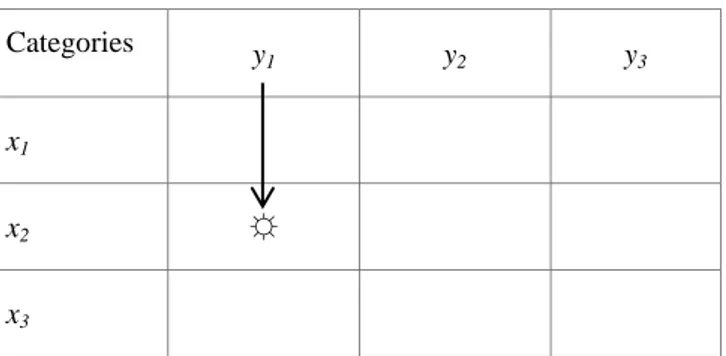
Consider the two categorical Variables, X and Y. Crossed, they span the X × Y contingency table with I rows and J columns. Now, suppose Category xi constitutes the origin of an effect, that is, an event, and Category yj, another event, is on the outcome side, with i = 1, …, I, and j = 1, …, J. This scenario is exemplified in the 3 × 3 Table 1, in which X is the row-variable and Y the column-variable. In this example, the direction of effect goes from x2 to y1.
Table 1. Direction of effect goes from x2 to y1
Categories y 1 y2 y3 x1 x2 ☼ x3
The cell frequencies in Table 1 (not given in this illustra-tion) would be m11, m12, …, m33.The arrow in Table 1
indi-cates the hypothesized direction of effect. In a research context in which causal hypotheses are examined, the hy-pothesis depicted in Table 1 could be that Event x2 is the cause of Event y1. If this hypothesis can be retained, Cell 2 1 contains more cases than Cells 2 2 and 2 3.
It should be noted that (1) there is more than one way to confirm this hypothesis, and (2) expectancies are to be tak-en into account. Specifically, several models and measures can be considered, and several ways can be considered to define expected values for models. In the present article, we focus on the latter. More detail follows in the sections on measures and models.
As was discussed by Wiedermann and von Eye (2015b), retaining a hypothesis of direction dependence is defensible in particular when (1) the hypothesis can be confirmed and (2) the opposite direction of effect can be refuted. Table 2 displays the scenario for the opposite direction of effect, that is, when the effect goes from y1 to x2.
Table 2. Direction of effect goes from y1 to x2
Categories y
1 y2 y3
x1
x2 ☼
x3
The arrow indicates the hypothesized direction of effect again. Here, when causal hypotheses are examined, it is posited that Event y1 is the cause of Event x2. If this hy-pothesis can be retained, Cell 2 1 contains more cases than Cells 1 1 and 3 1. Most important for the discussion in this article, there is asymmetry in these two hypotheses in that the comparison cells for the first hypothesis, 2 2 and 2 3, are constituted by the remaining cells of the outcome variable, Y. For the second hypothesis, the comparison cells, 1 1 and 3 1, are constituted by what now is the outcome variable, X.
Cell 2 1 – it could be called the hit cell (cf. Froman & Hubert, 1980; Hildebrand, Laing, & Rosenthal, 1977) – constitutes the intersection of the hypotheses of interest. In each case, the hit cell contains more cases than some func-tion (e.g., the mean) of the comparison cells in the corre-sponding rows and columns, or, to use the example in the two tables again, m21 > f (m22, m23) in Table 1, and m21 > f(m11,
m31) in Table 2. Thus, studying these frequency distributions
can be informative when discerning whether the directional effect X → Y, the reverse effect Y → X, both, or neither holds for the cross-classification table. When, in support of the hypothesis that the direction of effect goes from x2 to y1, Cell 2 1 is large, there is also an increased probability, that this is also in support of the hypothesis that the direction of effect goes from y1 to x2. Simulations presented later in this article will show how likely this is to occur. We now review measures that can be considered when testing directional hypotheses. This is followed by a description of the log-linear models that can be used to test hypotheses com-patible with direction of effect.
Common Measures of Association
In this section, we review three measures that can be used to quantify the magnitude of association in the cate-gorical data domain and point at potential drawbacks when assessing direction of effect. The measures are the Pearson X2, the odds ratio, and Hildebrand et al.'s (1977) measure Del, a measure of proportionate reduction in error.
For tables of any size, Pearson's X2 can be used to test the null hypothesis that the variables that span the cross- classification under study are independent. When a direc-tional effect is reflected in the frequency distribution, there
13 will be no independence, and the test will respond. How-ever, there are many ways to deviate from independence, directional effect being just one of them. Therefore, results that are based on this test will rarely be conclusive when direction dependence hypotheses are examined from an event-based perspective.
The odds ratio, very popular in epidemiological research, is a relative of the log-linear interaction (see Goodman, 1991). It is estimated by 21 12 22 11
m
m
m
m
,where the m.. are the cell frequencies in a 2 × 2 table. The odds ratio assesses the strength of an interaction in a 2 × 2 table. In Pearson's X2, the test statistic is weighted by the marginal totals. The statistic is, therefore, marginal- dependent (Goodman, 1991). The odds ratio is not weighted by the marginal totals and is, therefore, marginal-free. Proportional changes in the marginal probabilities will result in a different X2, but in an unchanged odds ratio. Because of this difference, Pearson's X2 and the odds ratio can suggest different statistical conclusions (for an illustration, see von Eye, Spiel, & Rovine, 1995). However, the odds ratio is symmetric as well. Therefore, directional hypotheses can rarely be tested with the odds ratio in a conclusive way in non-experimental studies. In tables that are larger than 2 × 2, the odds ratio can be employed in the context of decomposition of effects (see von Eye, & Mun, 2013).
Hildebrand, et al.'s (1977) Del measure can be traced back to Goodman and Kruskal’s (1954) asymmetric measure of similarity. Del is
ij ij ij ij ij ijm
m
ˆ
1
where ωij indicates hit cells, with ωij = 1 for hit cells and ωij = 0 otherwise. mij are the observed and
m
ˆ
ijare the expected cell frequencies. Main effect models and null models have been discussed for estimation. Considering that the summa-tion for both, S1 and S2, goes over the entire table, oneob-tains the same result for a hit cell for a directed effect and the effect that goes in the reverse direction. Therefore, and as for Pearson's X2 and the odds ratio, Del is symmetric, and, thus, unable to distinguish between direction of effect in opposite directions. Still, the measure should also re-spond in cases in which direction of effect exists that man-ifests in interaction-type relations in a table, but decisions will rarely be conclusive. For an analysis of the characteris-tics of Del, see for example von Eye and Sörensen (1991).
Log-linear Representations
In this section, we provide log-linear representations of the hypotheses discussed in the previous sections. Consider
the general log-linear model,
W
m
log
,where m is the vector of the estimated expected cell frequencies of the cross-classification under study, W is the design matrix, also called indicator matrix, and λ is the parameter of model vectors (see Agresti, 2013; von Eye & Mun, 2013). In the odds ratio test discussed in the previous sections, raw frequencies were compared with each other, without consideration of the row and column marginal probabilities. The base model was, thus, the log-linear null model. In the contexts of assessing rater agreement and prediction analysis, this approach has been discussed by Brennan and Prediger (1981). Alternatively, the main effects of the variables that span the cross-classification under study can be considered. Pearson’s X2 is based on a log-linear main effect model (see von Eye & Mun, 2013), and so is Cohen’s (1960) measure of rater agreement, kappa. The alternative of considering main effects is most meaningful when sampling is multinomial. Because the proposed approach relies on testing the (in)equality of the number of cases of a hit cell and the corresponding comparison cells, adjusting for main effects (i.e., potential heterogeneity of marginal distributions) is important to avoid biased direction dependence decisions.
Considering first the null model as the base model, we develop the models of interest from the model log m = 1 λ. where 1 is a vector of 1s. The design matrix of this model contains just one column, that is the constant vector. In a 2 × 2 table, the first hypothesis, that is, the hypothesis x1 → y1, can be expressed by a vector that contains a 1 for the hit cell and a –1 for the comparison cell. The design matrix thus becomes, when Cell 1 1 is the hit cell,
0
0
1
1
1
1
1
1
W
when effect coding is used. This model is non-standard (Mair & von Eye, 2007), but the design matrix is still orthogonal. Adding the vector for the reverse direction of effect hypothesis yields the matrix
0
1
0
1
0
0
1
1
1
1
1
1
W
This model is non-standard as well, but the vectors are no longer orthogonal which can render parameter interpretation problematic (Mair & von Eye, 2007; Rindskopf, 1999; von Eye & Mun, 2013).
von Eye & Wiedermann: Direction of effects in categorical variables
14 von Eye, Schuster, and Rodgers (1998) proposed a transformation that results in an orthogonal design matrix and parameter interpretation as intended by the design matrix before transformation. A summary of this transformation, which is known as the Schuster transformation, is given in Appendix A.
Alternatively, a hierarchy of log-linear models can be considered. In this hierarchy, the original direction dependence hypothesis is tested first, using the first of the two design matrices presented here. In a second step, the second contrast vector is added and the model is re- estimated. These two models are hierarchically related to each other. The ΔX2-test can be used to determine whether
adding the second vector improves the model. If this is the case, the second direction dependence hypothesis can be retained.
The model that contains both vectors will yield the same results, regardless of the order of the two vectors in the model. However, the evaluation of the individual contrasts in a hierarchy of models does depend on the order they are included in the design matrix, because they are not orthogonal. Therefore, a hierarchy of models is most useful when there clearly is an a priori direction dependence hypothesis, and the reverse direction hypothesis is tested only to rule out (or establish) the reverse direction of effect. This is in accordance with the procedure proposed by Wiedermann and von Eye (2015b). Specifically, one has found empirical evidence for the model X → Y when the model term representing the hypothesis X → Y is needed to explain the data (i.e., when log m = λ + λY→X + λX→Y represents the data better than log m = λ + λ Y→X) and, at the same time, the model term representing Y → X is not needed to explain variable associations (i.e., log m = λ + λY→X
+ λX→Y does not outperform log m = λ + λ X→Y). Before moving to the simulations and the data example, we first discuss identifiability of models and, second, examine the performance of such models in a simulation. As the above design matrices suggest, there will always be at least one degree of freedom left for statistical testing (unless covariates or other special effects are considered). When the main effects of the variables that span the cross-classification are also considered (which is recommended in multinomial sampling), the base model is not the null model but the main effect model. In a 2 × 2 table, this model comes with three vectors in the design matrix and, thus, one degree of freedom. Adding just one of the direction dependence hypothesis vectors renders this model saturated. Adding both renders the model over- identified.
In larger tables, the main effect model becomes a candidate for modeling direction of effect hypotheses. This applies whenever the main effect model comes with more than 2 degrees of freedom. Consider the case of three binary variables (X, Z, Y) that span a 2 × 2 × 2 table and assume that Cell 2 2 2 represents the hit cell. If the co-occurrence of X and Z causes Y, i.e., {X, Z} → Y, then the Cell 2 2 2 should
contain more cases than Cell 2 2 1. Reversely, if Y causes the co-occurrence of X and Z, i.e., Y → {X, Z}, then Cell 2 2 2 should contain more cases than the three Cells 1 1 2, 1 2 2, and 2 1 2. The design matrix for these two competing models can be written as
1
1
1
1
1
1
0
1
1
1
1
1
3
/
1
0
1
1
1
1
0
0
1
1
1
1
3
/
1
0
1
1
1
1
0
0
1
1
1
1
3
/
1
0
1
1
1
1
0
0
1
1
1
1
W
where the first column refers to the model intercept, columns 2 – 4 represent the main effects of X, Z, and Y, and the last two columns test the hypotheses {X, Z} → Y and Y → {X, Z}. Following the decision rules described above, one has found empirical support for a causal theory of the form {X, Z} → Y if (1) the model log m = λ+ λX + λZ + λY+ λ XZ→Y+ λY→XZ outperforms the model log m = λ + λX + λZ + λY+ λY→XZ in terms of model fit (i.e., the model term representing {X, Z} → Y is needed to explain variable associations) and, at the same time, (2) log m = λ + λX + λZ + λY+ λ XZ→Y + λY→XZ and log m = λ+ λX + λZ + λY+ λY→XZ do not differ in terms of model fit (i.e., the directionally reversed model term Y → {X, Z} does not contribute to explaining variable associations). Again, ΔX2
-tests can be used to test potential improvement of model fit. Because the main effects are considered in all three models, directional dependence decisions do not depend on possibly heterogeneous marginal distributions.
In the following section, we present results from two simulation studies. The studies were performed to explore the characteristics of the proposed approach and the performance of the proposed log-linear modeling approach under various conditions.
Monte Carlo Simulations
In this section, we present results from two simulation studies. In the first, we examine the number of events that reflect patterns of results. In the second study, we ask questions concerning the performance of log-linear models that can be specified to test event-based hypotheses that are compatible with direction dependence.
Simulation 1: Relative Frequencies of Direction Dependence Patterns
In the first simulation, cross-classifications of size 2 × 2 and 4 × 4 were created. For each size, 50,000 cross-
15 classifications were created using the uniform random number RANDOM_NUMBER available in the FORTRAN compiler Microsoft Developer Studio. In both, the 2 × 2 and the 4 × 4 cross-classifications, the hit cell was positioned at Cell 2 1.
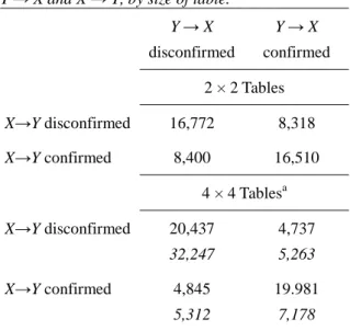
We now examine the 100,000 tables under the following question: To what degree are the comparisons of the hit cell frequency with the row and the column frequencies dependent? To answer this question, we cross the two variables that represent the numbers of instances in which the first (X → Y) and the reverse-direction hypotheses (Y → X) are numerically confirmed versus disconfirmed. Table 3 displays the results, by size of cross-tabulation. In the 2 × 2 tables, the hit cell is compared with the comparison cell, for both hypotheses. In the 4 × 4 tables, the hit cell is compared with the average frequency of the corresponding comparison cells.
Table 3. Cross-tabulation of cases of (dis)confirmed Y → X and X → Y, by size of table.
Y → X disconfirmed Y → X confirmed 2 × 2 Tables X→Y disconfirmed 16,772 8,318 X→Y confirmed 8,400 16,510 4 × 4 Tablesa X→Y disconfirmed 20,437 32,247 4,737 5,263 X→Y confirmed 4,845 5,312 19.981 7,178 a
Frequencies in italics calculated under the criterion that the hit cell be greater than each of the comparison cells; frequencies in regular type face calculated under the criterion that the hit cell be greater than the average of the comparison cells
Table 3 shows a clear picture. For cross-classifications of size 2 × 2, the majority of comparisons indicates that the direction dependence hypotheses are either not supported at all (Cell 1 1) or supported as pointing in both directions (Cell 2 2). More specifically, about twice as many comparisons suggest that the two comparisons lead to the same result as comparisons that lead to different results. This result is not surprising. When a cell is greater than its comparison cell in the same row, there is an elevated probability that it is also greater than its comparison cell in the same column. Accordingly, when a cell is smaller than its comparison cell in the same row, there is an elevated probability that it is also smaller than its comparison cell in the same column. Comparisons in support of one of the two direction
dependence hypotheses are half as likely, in either direction. In other words, under multinomial sampling, looking at the three cells that are involved in the test of a directional effect in a 2 × 2 table, these results confirm the a priori calculations that can easily be performed. Specifically, in such a scenario, the probability that the hit cell is the largest is exactly 1/3, the probability that it is the smallest is also exactly 1/3. The probability that the hit cell is the second largest when a given other cell is the largest is exactly 1/6. Table 3 shows only minor deviations from these probabilities. These differences are due to simulation errors. With larger simulation samples, these differences will decrease.
For cross-classifications of size 4 × 4, an even more extreme pattern results. For tables of this size, comparisons supporting the same decision for both direction dependence hypotheses are about 4.25 times as likely as comparisons that suggest that the support for just one of the directional dependence hypotheses. When individual cells are compared, that is, when the question is asked whether the hit cell is the largest of all comparison cells, similar calculations can be performed as for 2 × 2 tables. For instance, the probability that the hit cell is the largest is 1/7, and the probability that it is the smallest is 1/7 as well. In all, the simulated results correspond very closely with the exact calculations.
This result can be seen as in contrast with the results that suggest that, in Configural Frequency Analysis (CFA; Lienert, 1968; von Eye, 2002; von Eye & Gutiérrez-Peña, 2004), type- and antitype decisions are more dependent upon each other in smaller than in larger tables. von Weber, Lautsch, and von Eye (2003) showed that, when the expected cell frequencies in a 2 × 2 table are estimated under the model of first order CFA, that is, a log-linear main effect model, only the first CFA test can be expected to keep the a priori specified α level. The outcomes of the second, third, and fourth CFA tests in the 2 × 2 table are completely dependent upon the outcome of the first test. Krauth (2003) showed that the number of different patterns of types and antitypes increases as the size of a table increases, but that the tests in a CFA never become completely independent.
One explanation of this contrast between direction dependence analysis and CFA is that, in CFA, observed frequencies are compared with expected frequencies, both of which sum to the same subtables or marginal frequencies. Here, the comparison is between observed frequencies, and the probability of one frequency being greater than the average in the rest of a row while being smaller than the average in the rest of the corresponding column evidently decreases as the number of cells in a row/column increases. This applies when the null model is used as a base model, but it can also apply when the main effect model is used. In the following section, we present a simulation study on the performance of specific log-linear models.
There are two main conclusions that can be drawn from the first simulation. First, the hypotheses that posit opposite
von Eye & Wiedermann: Direction of effects in categorical variables
16 direction of effects become increasingly unlikely to be distinguishable as the number of categories of the variables increases that span a cross-classification. Table 3 shows that, in 2 × 2 tables, the probability that just one of the directed hypotheses can be retained is 0.5. The probability that just one of the two hypotheses can be retained in 4 × 4 tables is about 0.25. As tables increase in size, this probability decreases even more.
Second, the various options to compare the hit cell with the comparison cell(s) are distinguishable only when a cross-classification is at least of size 3 × 3. For example, when the direction of effect hypothesis is retained only when the hit cell is greater than each of the hit cells (in Table 3, the hypothesis was retained when the hit cell was greater than the average of the average of the comparison cells), one obtains the results given in italics in the bottom panel of Table 3. Thus, when researchers entertain hypotheses that distinguish between these two and (possibly) other criteria, they need to resort to 3 × 3 or larger tables, even if the probability of retaining just one of the direction of effect hypothesis is reduced in tables larger than 2 × 2.
Simulation 2: Performance of Log-Linear Model Selection
To analyze the performance of the proposed model selec-tion procedure, a second simulaselec-tion experiment was per-formed. This study was designed to mimic the situation in which researchers ask questions concerning direction of effect in multivariate data settings. The “true” data- generating mechanism of three binary variables X, Y, and Z followed a logistic regression of the form
XZ
Z
X
Z XZ X
01
log
)
(
logit
where π denotes the probability of Y = 1 (1 – π being the probability of Y = 0), and the β parameters denote the effects of the “true” predictors (X and Z) on the “true” outcome Y. Specifically, βXZ represents the causal effect associated with the hit cell {X = 1, Z = 1, Y = 1} and was varied from 0 to 1 in increments of 0.25. The intercept β0 was fixed at zero and
the main effects (βX and βZ)were either 0 or 0.5. Note that the case of βX =βZ = βXZ = 0 represents the null scenario which was used to assess the Type I Error behavior of the proposed model selection procedure.
Cases of non-zero parameters refer to scenarios where a true causal effect of X and Z on Y exists, which was used to evaluate the statistical power of the approach. Base rates for X and Z were Pr(X = 1) [Pr(Z = 1)] = 0.3 [0.3], 0.3 [0.5], 0.5 [0.5], 0.7 [0.5], and 0.7 [0.7]. Sample sizes were n = 50, 100, 200, and 500 (the selection was guided by Cressie,
Pardo, and del Carmen Pardo, 2003; and Stelzl, 2000). Simulation factors were fully crossed for both, the Type I Error and the power simulation. The Type I Error simula-tion consisted of 4 (sample size) × 5 (base rates) = 20 sim-ulation conditions, the power simsim-ulation consisted of 4 (sample size) × 5 (base rates) × 5 (effect size) = 100 condi-tions. For each condition, 1,000 samples were generated. For each sample, the three models
log m = λ+ λX + λZ + λY+ λY→XZ (Model I), log m = λ+ λX + λZ + λY+ λXZ→Y (Model II), and log m = λ+ λX + λZ + λY+ λXZ→Y + λY→XZ (Model III) were estimated, and ΔX2
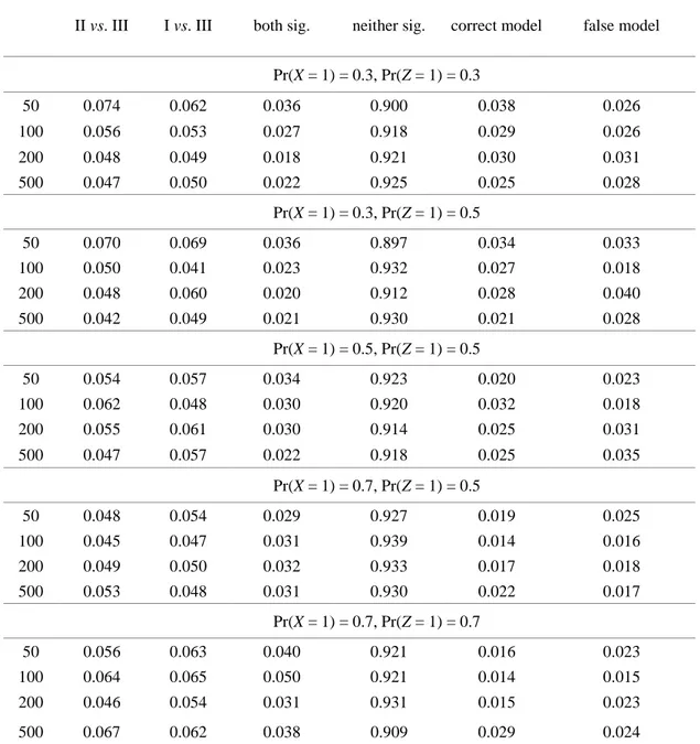
-tests were used to compare model fits of I vs. III and II vs. III (the arrows in the model equations indicate the parameters that were estimated for the directional hypotheses). For each condition, we retained the number of significant results using a nominal significance level of 5%.
Type I Error Behavior: The first two columns of Table 4 show the probabilities of rejecting the null hypothesis of model fit equality for Models I vs. III and II vs. III. Each cell gives the portion of significant ΔX2-tests based on 1,000 generated samples. For example, when n = 100 and Pr(X = 1) = 0.3, Pr(Z = 1) = 0.3, 62 ΔX2-tests indicated a significant model fit improvement when comparing Model I and III. In general, Type I Error rates of both ΔX2
-tests reside within Bradley's (1978) robustness interval of 2.5 – 7.5%. The tests are, thus, able to protect the nominal significance level and only reject the null hypotheses by chance. Columns 3 – 6 show the probabilities of combined statistical decisions of the two ΔX2-tests, i.e., both model comparisons show significant model differences, neither comparison shows a significant model difference, and either {X, Z} → Y is selected over Y → {Z, X} or vice versa.
When neither/both ΔX2
-tests are significant, no directional decision is possible based on the proposed decision rule. The results suggest that, in general, observed probabilities do not depend on base rates and sample size. The portion of non-significant results for both model comparisons is always larger than 90% and the probabilities of selecting {X, Z} → Y or Y → {Z, X} are close to α/2 = 2.5%, as expected. In other words, either selecting {X, Z} → Y or Y → {Z, X} is observed by chance and is in line with the overall nominal significance level of 5%. Overall, we conclude that, as expected, in the null case, no distinct decisions can be made based on the proposed model selection procedure.
17
Table 4. Empirical Type I Error rates of ΔX2-tests (Model I: log m = λ+ λX + λZ + λY+ λY→XZ; Model II: log m = λ+ λX + λZ + λY+ λXZ→Y; Model III: log m = λ+ λX + λZ + λY+ λXZ→Y+ λY→XZ). Columns 1-2 give the relative frequencies of significant ΔX2
-tests when comparing Models II vs. III and Models I vs. III. Columns 3-6 give the portions of combined statistical decisions of the two ΔX2
-tests.
II vs. III I vs. III both sig. neither sig. correct model false model
Pr(X = 1) = 0.3, Pr(Z = 1) = 0.3 50 0.074 0.062 0.036 0.900 0.038 0.026 100 0.056 0.053 0.027 0.918 0.029 0.026 200 0.048 0.049 0.018 0.921 0.030 0.031 500 0.047 0.050 0.022 0.925 0.025 0.028 Pr(X = 1) = 0.3, Pr(Z = 1) = 0.5 50 0.070 0.069 0.036 0.897 0.034 0.033 100 0.050 0.041 0.023 0.932 0.027 0.018 200 0.048 0.060 0.020 0.912 0.028 0.040 500 0.042 0.049 0.021 0.930 0.021 0.028 Pr(X = 1) = 0.5, Pr(Z = 1) = 0.5 50 0.054 0.057 0.034 0.923 0.020 0.023 100 0.062 0.048 0.030 0.920 0.032 0.018 200 0.055 0.061 0.030 0.914 0.025 0.031 500 0.047 0.057 0.022 0.918 0.025 0.035 Pr(X = 1) = 0.7, Pr(Z = 1) = 0.5 50 0.048 0.054 0.029 0.927 0.019 0.025 100 0.045 0.047 0.031 0.939 0.014 0.016 200 0.049 0.050 0.032 0.933 0.017 0.018 500 0.053 0.048 0.031 0.930 0.022 0.017 Pr(X = 1) = 0.7, Pr(Z = 1) = 0.7 50 0.056 0.063 0.040 0.921 0.016 0.023 100 0.064 0.065 0.050 0.921 0.014 0.015 200 0.046 0.054 0.031 0.931 0.015 0.023 500 0.067 0.062 0.038 0.909 0.029 0.024
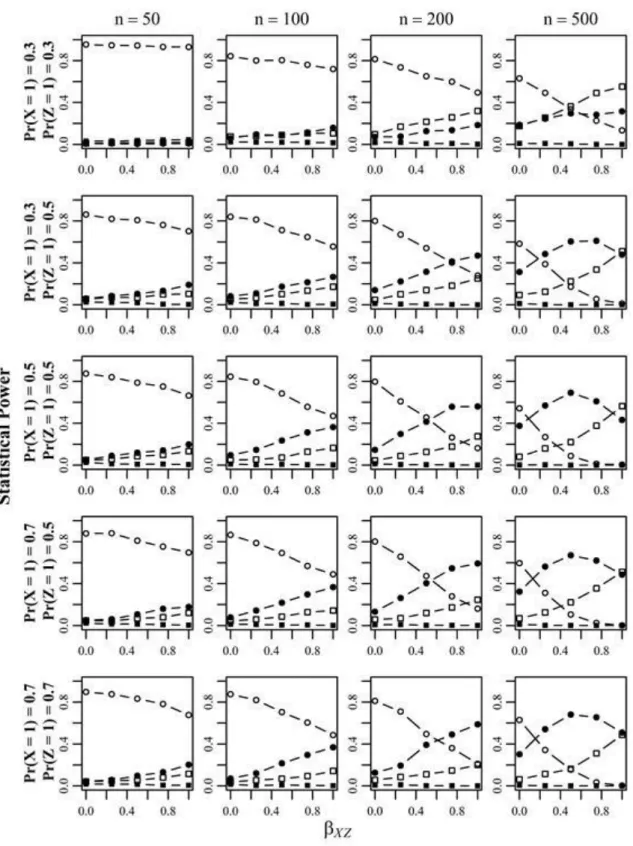
Statistical Power: Next, we focus on the statistical power of the procedure. Figure 1 shows the power of the two ΔX2-tests when comparing Models II vs. III (i.e., when
adding the effect assuming {X, Z} → Y) and Models I vs. III (i.e., adding the effect reflecting Y → {X, Z}). As expected, the test that evaluates II vs. III is more powerful than the competing procedure (I vs. III). In general, power increases with the magnitude of the causal effects and the sample size. Base rates of X and Z have almost no effect on the statistical power.
Figure 2 shows the empirical power curves for the combined statistical decisions. The power to select the correct model systematically increases with the magnitude
of the causal effect. Here, for large sample sizes (i.e., n = 500) an inverse U-shaped pattern is observed which can be explained by the fact that the power of model comparison I vs. III increases with large sample sizes and large causal effects. For these cases, the rates where both model comparisons are significant systematically increase. From a model prediction perspective, this implies that the additional effect Y → {X, Z} significantly contributes to reduce prediction error. However, from the perspective of causal explanation, any model that includes effects which treat the true outcome as an explanatory variable is directionally mis-specified by definition (for a discussion on predictive and explanatory modeling see Shmueli, 2010).
18
Figure 1. Observed power of the ΔX2-tests associated with the two competing log-linear model comparisons as a function of predictor base rates, sample size, and effect size. {XZ} → Y reflects the comparison Models II vs. III, Y → {XZ} reflects the comparison Models I vs. III. The x-axis gives the magnitude of the causal effect βXZ and the y-axis gives portion of significant ΔX2-tests based in the 1,000 generated samples.
19
Figure 2. Combined statistical decisions of ΔX2-tests associated with the two competing log-linear model comparisons. The x-axis gives the magnitude of the causal effect and the y-axis gives the portion of combined decisions of separate ΔX2-tests based on the 1,000 generated samples.
von Eye & Wiedermann: Direction of effects in categorical variables
20 Recall that the data-generating mechanism described above implies that both predictors, X and Z, are generated outside the model. Most important, the portion of erroneously selecting the mis-specified model is close to zero across all considered scenarios. Again, base rates only have a small effect on the power curves. Overall, we can conclude that, in particular for larger sample sizes (such as n ≥ 200), the algorithm is well-suited to identifying the direction of effect. Further, simulation results suggest that the proposed algorithm is capable of identifying the correct model (i.e., the fact that the true causal effect is transmitted from X and Z on Y) even when the “true” log-linear model is not among the candidate models (the log-linear model that corresponds to the true data-generating mechanism would be log m = λ+ λX + λZ + λY+ λXZ + λXY + λYZ + λXYZ, see Agresti, 2013; von Eye & Mun, 2013).
Data example
For the following data example, we use data from the European Social Survey (ESS, 2014). The main goals of the ESS include the measurement of attitudes, beliefs and behavior patterns in more than thirty European nations. The ESS aims at charting stability and change in social structure and attitudes in Europe, and depicting how Europe’s nations differ in their social, political and moral structures, and change over time. The survey includes a number of demo- graphic measures as well as a question about happiness of respondents. Here, we use just two of the several hundred variables (cf. von Eye & Wiedermann, 2016a): happiness and household income. Happiness was originally measured on a scale from 0 (extremely unhappy) through 11 (extreme- ly happy). Household income was originally measured in units of Euros. All sources of income were considered. In the public ESS data files, total income is given on a 10-point scale, where each scale point represents a decile of the population distribution. Refusals, don't know answers, and no answer cases were excluded from the following analyses. We selected the responses from the participants in Austria. A total of 1,795 respondents were thus available. Table 5 presents descriptive statistics of these two variables. Table 5. Descriptive statistics of happiness and income (ESS data; original scale scores).
How happy are you
Household's total net income, all sources
N of Cases 1,795 1,795 Minimum 0.000 1.000 Maximum 10.000 10.000 Arithmetic Mean 7.102 5.439 Standard Deviation 2.120 1.921 Skewness (G1) –0.755 –0.050 Kurtosis (G2) 0.169 –0.735
For the following analyses, we categorize both variables. Happiness was re-scaled as follows: Categories 1 through 4 = 1; Category 5 = 2; Category 6 = 3; Categories 9 and 10 = 4. Income was categorized as follows: Categories 1 through 3 = 1; Categories 4 and 5 = 2; Categories 6 and 7 = 3; Categories 8 through 10 = 4. Combining categories is, in the present example, needed for two reasons. First, re- ducing the number of categories from 10 to 4 results in a smaller cross-classification. Accordingly, the number of possible hypotheses is reduced and the reader has an easier time to re-calculate the example. Second, the table that resulted from crossing the original categories was sparse, in particular in those sectors in which high levels of happiness were combined with low income, and vice versa. The goodness-of-fit tests that are used in log-linear modeling require expected cell frequencies that are larger than 0.8 (see Larntz, 1978) to approximate the theoretical χ2 distribution, and there was a relatively large number of cells with expected frequencies smaller than 0.8. Table 6 displays the cross-classification of the thus re-scaled variables Happiness (H) and total household Income (I). Table 6. Cross-classification of the categorized scales of Happiness (rows) and Income (columns).
Income Happi-ness 1 2 3 4 Total 1 143 95 54 140 432 2 126 80 60 131 397 3 121 97 74 181 473 4 106 92 110 185 493 Total 496 364 298 637 1,795
We analyze the data in Table 6 and ask whether money makes one happy or, alternatively, whether happier respondents garner higher incomes. We propose the following models. For the first hypothesis (“money makes you happy”), there are two hit cells. The first is Cell 3 4 (n = 181), the second is Cell 4 4 (n = 185). Evidently, these are the largest cells. The cells disconfirming the first hypothesis are Cells 1 4 (n = 140) and 2 4 (n = 131).
To analyze the cross-classification in Table 6, we first calculate a Pearson's X2 = 34.11 (df = 9; p < 0.01). This result suggests a significant association between happiness and income. One could be tempted to interpret this result as in support of the hypothesis that money makes one happy. However, considering that Pearson's X2 is symmetric, the reverse-direction hypothesis cannot be discarded, that is, that happier individuals garner higher incomes. To arrive at a conclusion concerning the status of the original hypothesis and its reverse, we compare the hit cells, 3 4 and
21 4 4, with cells 1 4 and 2 4 (for the original hypothesis) and 4 1 and 4 2 (for the reverse-direction hypothesis)1. In the following paragraphs, we specify the log-linear models with which we test these two hypotheses. In all, we estimate four models. These are two models each that contain the directed effect hypotheses without and with the Schuster transformation.
The design matrix for the model that includes the main effects and both direction dependence hypotheses is, in effect coding,
1
1
1
1
1
1
1
1
1
0
0
1
0
0
1
1
1
1
1
0
0
1
0
1
1
1
1
1
0
0
0
1
1
1
1
1
0
1
1
1
1
1
0
0
1
0
0
1
0
0
1
0
0
1
0
0
0
1
0
1
0
0
1
0
0
0
0
1
1
0
0
1
0
1
1
1
1
0
1
0
1
0
0
1
0
0
0
1
0
1
0
0
0
1
0
0
1
0
1
0
0
0
0
1
0
1
0
1
0
1
1
1
1
0
0
1
1
0
0
1
0
0
0
0
1
1
0
0
0
1
0
0
0
1
1
0
0
0
0
1
0
0
1
1
W
The first column in this matrix represents the constant vector. The following six columns represent the main effects of the two 4-category variables that span the cross-classification given in Table 6. The eighth column represents the first hypothesis, according to which people who earn more money are happier. The reverse-direction hypothesis is represented in the last column. According to his hypothesis, happier people earn higher salaries.
Asking whether money makes one happy or vice versa, we first estimate the model with the design matrix that
1
Please notice that, in order to specify a symmetric direction and reverse-direction hypothesis, Cell 4 3 should be considered a comparison cell as well. When Cell 4 3 is considered a
comparison cell, the two directed effect vectors are {0 0 0 0 0 0 0 0 –1 –1 1 1 –1 –1 1 1}’ and {0 0 –1 –1 0 0 –1 –1 0 0 1 1 0 0 1 1}’. The goodness-of-fit LR-X2 for this model is 14.08 (df = 7; p = 0.05). Parameter interpretation for this model, however, can be complicated because estimation of the second directed effect parameter suffers from local singularities that are due to the correlation between the two directed effect vectors (r = 0.50).
cludes the first eight vectors of this design matrix (i.e., con-sidering all main effects and the vector representing money → happiness). We assume multinomial sampling and obtain the overall goodness-of-fit LR-X2 = 28.51, a value that makes us reject the model (df = 8; p < 0.001). Considering, however, that, although we are not in the process of model fitting, we tentatively ask whether the parameter of interest is significant. This is clearly the case (λ = 0.11; se = 0.040; z = 2.293; p = 0.022). Next, we compare this model to the one that uses all nine vectors of the design matrix, that is, we ask whether the vector happiness → money contributes to ex-plaining the data. We obtain ΔX2
= 11.69 which suggests that the model significantly improved (df = 1, p < 0.001). Thus, we cautiously conclude that there is support for the hy-pothesis that happier people garner higher income. However, to complete the analysis, we have to empirically confirm that the vector money → happiness vector does not improve the model that consists of the main effects and the reverse cau-sation vector happiness → money. We, therefore, use the last vector in the design matrix instead of the second-to-last and re-estimate the model. We obtain the overall goodness-of-fit LR-X2 = 19.71, a value that makes us reject the model again (df = 8; p < 0.001). The parameter for the reverse hypoth-esis is also significant (λ = 0.230; se = 0.061; z = 3.737 ; p < 0.001). Comparing this model with the one using all nine vectors of the design matrix leads to a non-significant change in model fit (ΔX2
(1) = 2.88, p = 0.090). This result suggests that there is support for the hypothesis that happier people garner more money.
Discussion
In this article, we propose a new way of examining direction dependence hypotheses. Instead of looking at marginal distributions, we inspect frequency distributions inside cross-classifications. It is shown that a direction dependence hypothesis and its reverse, that is, the hypothesis that proposes dependence in the opposite direction, can both be examined in the same table. The intersection of these two hypotheses is the hit cell, that is, the cell in which those events are found that support one direction dependence hypothesis, its reverse, or both. The tests of a direction dependence hypothesis and its reverse are, to a certain degree, dependent upon each other. The degree of dependence varies with the size of the cross-classification. In smaller tables, there is less dependence than in larger tables. The degree of dependence also varies with the criterion used for the comparison of the hit cells with the comparison cells, and with the symmetry of the directed hypotheses.
However, and this is one of the most important characteristics of the method proposed here, a direction dependence hypothesis and its reverse are not considered as necessarily competing. Instead, four outcomes of testing hypotheses that are compatible with direction dependence
von Eye & Wiedermann: Direction of effects in categorical variables
22 are considered. The first outcome is that the first direction dependence hypothesis prevails (note, that the order in which the direction dependence hypotheses are tested is of no importance; results will stay unchanged when the order is reversed). The second is that the reverse of the first hypothesis prevails instead. The third outcome is that both hypotheses prevail, and the fourth possible outcome is that neither prevails. Depending on context, each of these outcomes can have a meaningful interpretation. This pattern of results is in accordance with the recent literature on direction dependence analysis with metric variables (cf. Wiedermann, Hagmann, & von Eye, 2014; Wiedermann, & von Eye, 2015). However, the hypotheses that are tested with the methods proposed here and the currently discussed methods for metric variables differ fundamentally. In the literature for metric variables, univariate distributions of variables or residuals are examined. Here, special interactions are examined.
It is interesting to ask how the methods presented here compare to methods created in the context of the development of methods for the analysis of direction dependence hypotheses in metric variables. In addition, one might ask how the results in the empirical data example compare to results one could create using existing methods for the analysis of direction dependence in metric variables. The answers to these questions are important as they allow one to position the methods proposed in this article in the canon of methods for direction dependence analysis.
An answer to these questions can be given as follows. Existing methods for direction dependence analysis in metric variables focus on univariate outcomes. Specifically, these methods decompose the distribution of the outcome variable into the systematic part, that is, the Xβ part of the linear regression model, and the random part, that is, the ε, the error part of the model. When the regression model is properly applied, the distribution of the outcome variable, Y, is less skewed than the distribution of X, when X is skewed (see Dodge, & Rousson, 2000, 2001; Wiedermann, et al., 2014, 2015b). First developments of methods of direction dependence analysis for categorical variables assimilated these ideas (see von Eye, & Wiedermann, 2016). The focus of these methods is the univariate distribution of outcome variables that are crossed with predictors. That is, the focus is on marginal distributions or, for both, metric and categorical variables, main effects.
In contrast, the present article focuses on characteristics of frequency distributions that cannot be found in marginal distributions but inside the table. To test hypotheses about these characteristics, special interactions are specified and made part of the model. Marginal distributions are part of the model, for two reasons. First, the model must not fail because marginal distributions that are not critical to the hypotheses were not included. If this is the case, conclusions about the hypotheses are not possible. Second, a model that focuses on special interactions does not make any assumptions on marginal distributions. Therefore, any
distributional characteristic of marginals is admissible. Now, a re-analysis of the data example using current methods for direction dependence analysis for metric data certainly can be done. However, a comparison of results would not be conclusive with respect to the performance of existing methods for metric variables in comparison to the methods for categorical variables proposed in this article. This comparison would contrast main effect models for metric variables with interaction models for categorical variables. In other words, focus of analysis would be confounded with scale characteristic of variables. Still, analyses that focus on main effects and analyses that focus on interactions can be performed in a complementary way.
Extensions: In a fashion parallel to Hildbrand et al.'s (1977; cf. von Eye & Brandtstädter, 1988) prediction analysis or confirmatory prediction CFA (see von Eye, & Rovine, 1994), the present approaches can straightforwardly be extended to the multiple - multivariate case. An example of a prediction of events could, when three predictors and two outcome variables are used, be expressed by. x1
x2
x3 → y1
y2 In this example, each of the threeevents on the predictor side must occur for the prediction to take place. In addition, each of the two events on the outcome side must occur for the prediction to come true. In the cross-classification of the five variables involved in this prediction, Cell 1 2 3 1 2 is the hit cell and the cells that do not represent events y1
y2 when x1
x2
x3 was observedare the comparison cells. For the reverse hypothesis, the hit cell is the same, and the cells that do not represent x1
x2
x3 when y1
y2 was observed are the comparisoncells. Details of multivariate extensions of the present approach will be explicated in a different context. In the second of the above simulation studies, two predictors and one outcome were examined already.
The vectors in the design matrix that represent the direction dependence are not orthogonal. Therefore, it can be hard to interpret the estimated parameters when these vectors are in the model simultaneously. Therefore, we discussed a hierarchical log-linear modeling procedure. In this procedure, the more important direction dependence hypothesis is included in the model first. In this case, its parameter can be interpreted. The contribution of the second direction dependence hypothesis can be estimated by the X2 difference between the first and the second model, the latter containing both directed effect vectors. When the direction dependence vectors and the main effect vectors are non-orthogonal, we recommend using the Schuster transformation.
There is an additional caveat that should be taken into account when the log-linear approach to hypothesis testing is tested. Because of the non-orthogonality of the vectors of some of the nonstandard models that are specified in direction dependence analysis, problems with parameter estimation can prevent the data analyst from deriving conclusions about the hypotheses that are studied. To illustrate, consider a 3 × 3 cross-classification. Let the model
23 that is estimated contain the main effects of both variables. Let Cell 1 3 be the hit cell, and let both directional hypotheses be estimated in the same model. The design matrix for this model is
0
0
1
1
1
1
1
0
0
1
0
1
1
1
0
1
0
1
1
1
1
0
0
1
1
1
0
1
0
0
1
0
1
0
1
0
1
0
1
1
0
1
1
0
1
1
0
1
1
1
0
1
0
0
1
1
2
2
0
1
0
1
1
W
In this design matrix, vectors are correlated. Specifically, the two vectors in each main effect are correlated to 0.5, and the two directional effect vectors (the last two in the matrix) are correlated to 0.667. Most software packages evince problems with the estimation of this model. This result applies even when other estimation methods are used than the standard maximum likelihood. In contrast, when design matrices are orthogonal, no estimation problems arise.
Hypotheses of direction dependence are often specified in contexts of causality. The event based on which another event is predicted is often called the cause, and the outcome event is often called the effect. Without going into detail, we emphasize that causal hypotheses must be compatible with substantive theory as well as causality theory. Looking at causality theory, consider, for example, the very well-known theory that goes back to Hume (1777). Among the central elements of this theory is the principle of temporal priority. According to this principle, the cause must precede the effect in time. Other theories of causality, for example mechanistic theory (see, e.g., Williamson, 2011) or epistemic theory (Hall, 2016), do allow researchers to consider contemporaneous causal effects, even causes that lie in the future.
Now, when researchers test both direction dependence hypotheses, the original one and its reverse, temporal priority must be discussed very carefully, and the concept tested must be compatible with substantive and causal theory alike. More specifically, if it is considered possible that, when both direction dependence hypotheses are tested, the events under study can be assumed to be active simultaneously, the substantive model cannot be based on Hume's theory of causality. Another possibility is that temporal order is assumed. In this case, the first event may be observed occurring before the second, and this part of the model may be compatible with Hume's theory. The second event, however, that is, the effect of the first cause, is, when both direction dependence hypotheses are tested, also the
cause of the first event. That is, when there is temporal order and both direction dependence hypotheses are tested, one of the causes must meaningfully be placeable into the future of the first. This would be in contradiction with Hume's principle, and researchers can do much worse than considering another theory of causality.
Conceptual and theoretical elements of causality theory can also heavily impact the design of a study. When researchers specify a substantive causal process based on Hume’s (1777) causality theory and its proposition of temporal ordering of cause and effect, data from cross- sectional studies will not enable the data analyst to test hypotheses that are compatible with the underlying causality theory. Longitudinal data will be needed. In contrast, when epistemic or mechanistic causality theories (see, e.g., Williamson, 2011; Hall, 2016) are the building blocks for a substantive causality theory, cross-sectional data can be used to test hypotheses that conform to such theories.
In either case, the methods proposed here can be of use. The cross-sectional case was illustrated in the data example in the last section. The longitudinal case leads to a more complex situation because there is, at the least, a third variable to be considered in a model, that is, time. The resulting design will be parallel to the one suggested in the paragraph on multivariate extensions, above, with the exception that, in most circumstances, the variable time is neither considered an explanatory nor an outcome variable.
The current discussion led us to a very interesting juncture. We find ourselves at a point where social science substantive theory, statistical modeling, and philosophical theory must be compatible. More interdisciplinary work is needed to flesh out the ramifications of this situation (see Wiedermann & von Eye, 2016b).
References
Agresti, A. (2013). Categorical data analysis (3rd ed.). Hoboken, NJ: Wiley.
Bradley, J. V. (1978). Robustness? British Journal of Mathematical and Statistical Psychology, 31, 144-152. Brennan, R.L., & Prediger, D.J. (1981). Coefficient kappa:
Some uses, misuses, and alternatives. Educational and Psychological Measurement, 41, 687-699.
Cohen, J. (1960). A coefficient of agreement for nominal scales. Educational and Psychological Measurement, 20, 37-46.
Cressie, N., Pardo, L., & del Carmen Pardo, M. (2003). Size and power considerations for testing loglinear models using φ-divergence test statistics. Statistica Sinica, 13, 555 – 579.
Dodge, Y., & Rousson, V. (2000). Direction dependence in a regression line. Communications in Statistics: Theory and Methods, 32, 2053-2057. doi:
10.1080/03610920008832589
Dodge, Y., & Rousson, V. (2001). On asymmetric properties of the correlation coefficient in the regression setting. The
von Eye & Wiedermann: Direction of effects in categorical variables
24 American Statistician, 55, 51-54. doi:
10.1198/000313001300339932
Dodge, Y., & Yadegari, I. (2010). On direction of dependence. Metrika, 72, 139-150.
ESS: The European Social Survey. Retrieved on 9/30/2014 from http://www.europeansocialsurvey.org/about/index.html Froman, T., & Hubert, L.J. (1980). Application of prediction analysis to developmental priority. Psychological Bulletin, 97, 136 – 146.
Goodman, L.A. (1991). Measures, models, and graphical displays in the analysis of cross-classified data. Journal of the American Statistical Association, 86, 1085 – 1111. Goodman, L.A., & Kruskal, W.H. (1954). Measures of
association for cross-classifications. Journal of the American Statistical Association, 49, 732 – 764. Hildebrand, D.K., Laing, J.D., & Rosenthal, H. (1977).
Prediction analysis of cross-classifications. New York: Wiley.
Hall, N. (2016). Causation and the aim of inquiry. In W. Wiedermann & A. von Eye (eds.). Statistics and
causality: Methods for applied empirical research (pp. 3 – 30). Hoboken, NJ: Wiley.
Hume, D. (1777/1975). Enquiries concerning human understanding and concerning the principles of morals. Oxford: Clarendon Press.
Krauth, J. (2003). Type structures in CFA. Psychology Science, 45, 217 – 222.
Larntz, K. (1978). Small sample comparisons of exact levels for chi-squared goodness-of-fit statistics. Journal of the American Statistical Association, 73, 253 - 236. Lienert, G. A. (1968). Die "Konfigurationsfrequenzanalyse"
als Klassifikationsmethode in der klinischen Psychologie. Paper presented at the 26. Kongress der Deutschen Gesellschaft für Psychologie in Tübingen 1968. Mair, P., & von Eye, A. (2007). Application scenarios for
nonstandard log-linear models. Psychological Methods, 12, 139 – 156.
Rindskopf, D. (1999). Some hazards of using nonstandard log-linear models, and how to avoid them. Psychological Methods, 4, 339 - 347.
Shimizu, S., Hoyer, P. O., Hyvärinen, A., & Kerminen, A. (2006). A linear non-Gaussian acyclic model for causal discovery. Journal of Machine Learning Research, 7, 2003 - 2030.
Shimizu, S., & Kano, Y. (2008). Use of non-normality in structural equation modeling: Application to direction of causation. Journal of Statistical Planning and Inference, 138, 3483 – 3491.
Shmueli, G. (2010). To explain or to predict? Statistical Science, 25, 289-310.
Stelzl, I. (2000). What sample sizes are needed to get correct significance levels for log-linear models? - A Monte Carlo Study using the SPSS-procedure "Hiloglinear". Methods of Psychological Research Online 2000, 5, 2, 1 – 22. Sungur, E.A. & Çelebioglu, S. (2011). Copulas with
directional dependence property. Gazi University Journal
of Science, 24, 415 – 424.
von Eye, A. (2002). Configural Frequency Analysis - Methods, Models, and Applications. Mahwah, NJ: Lawrence Erlbaum.
von Eye, A., & Brandtstädter, J. (1988). Formulating and testing developmental hypotheses using statement calculus and non-parametric statistics. In P. B. Baltes, D. Featherman, & R. M. Lerner (Eds.), Life-span
development and behavior (Vol. 8, pp. 61-97). Hillsdale, NJ: Erlbaum.
von Eye, A., & DeShon, R.P. (2008). Characteristics of measures of directional dependence - A Monte Carlo study. Interstat,
http://interstat.statjournals.net/YEAR/2008/articles/0802 002.pdf
von Eye, A., & DeShon, R. P. (2012). Directional dependence in developmental research. International Journal of Behavioral Development, 36, 303-312. doi: 10.1177/0165025412439968
von Eye, A., & Gutiérrez-Peña, E. (2004). Configural Frequency Analysis - the search for extreme cells. Journal of Applied Statistics, 31, 981 – 997.
von Eye, A., & Mun, E.-Y. (2013). Log-linear modeling - Concepts, Interpretation and Applications. New York: Wiley.
von Eye, A., & Rovine, M. J. (1994). Non-standard log-linear models for orthogonal prediction: Configural Frequency Analysis. Biometrical Journal, 36, 177 - 184.
von Eye, A., Schuster, C., & Rogers, W.M. (1998). Modelling synergy using manifest categorical variables. International Journal of Behavioral Development, 22, 537 – 557.
von Eye, A., Spiel, C., & Rovine, M. J. (1995). Concepts of nonindependence in Configural Frequency Analysis. Journal of Mathematical Sociology, 20, 41 – 54. von Eye, A., & Sörensen, S. (1991). Models of chance
when measuring interrater agreement with kappa. Biometrical Journal, 33, 781 – 787.
von Eye, A., & Wiedermann, W. (2013). On direction of dependence in latent variable contexts. Educational and Psychological Measurement, 74, 5 - 30.
doi:10.1177/0013164413505863
von Eye, A., Wiedermann, W. (2016). Fellow scholars: let’s liberate ourselves from scientific machinery. Research in Human Development. doi:
10.1080/15427609.2015.1068062 (in press) (a)
von Eye, A., Wiedermann, W. (2016). Direction of effects in categorical variables - A structural perspective. In W. Wiedermann & A. von Eye (Eds.), Statistics and causality: Methods for applied empirical research (pp. 107 – 130), Hoboken, NJ: Wiley. (b)
Wiedermann, W., Hagmann, M., & von Eye, A. (2014). Significance tests to determine the direction of effects in linear regression models. British Journal of Mathematical and Statistical Psychology, doi: 10.1111/bmsp.12037
25 Wiedermann, W., & von Eye, A. (2015). Direction of effects
in mediation analysis. Psychological Methods, 20, 221 – 244. (a)
Wiedermann, W., & von Eye, A. (2015). Direction dependence analysis: A confirmatory approach for testing directional theories. International Journal of Behavior Development, 39, 570 – 580.
doi:10.1177/0165025415582056 (b)
Wiedermann, W., & von Eye, A. (2016). Statistics and causality: Methods for applied empirical research. Hoboken, NJ: Wiley . (b)
Wiedermann, W. & von Eye, A. (2016). Directional dependence in the analysis of single subjects. Journal of
Person-Oriented Research, 2, 20 – 33. (a)
Wiedermann, W., & Hagmann, M. (2016). Asymmetric properties of the Pearson correlation coefficient: Correlation as the negative association between linear regression residuals. Communications in
Statistics-Theory and Methods, 45(21), 6263-6283. Wiedermann, W., Artner, R., & von Eye, A. (2017).
Heteroscedasticity as a basis of direction dependence in reversible linear regression models. Multivariate Behavioral Research, 52(2), 222-241.
Williamson, J. (2011). Mechanistic theories of causality. Part I. Philosophy Compass, 6, 421-432. doi: