Corruption and Income Inequality : A study of the impact from different legal systems

(1)

J

Ö N K Ö P I N G

I

N T E R N A T I O N A L

B

U S I N E S S

S

C H O O L

JÖNKÖPING UNIVERSITY

C o r r u p t i o n a n d I n c o m e I n e q u a l i t y

A study of the impact from different legal systems

Bachelor thesis within Economics

Author:

Christian Johansson

Carl-Johan Lext

Tutor:

Per-Olof Bjuggren

Johanna Palmberg

Jönköping, May 2013

(2)

Acknowledgements

We would like to thank our tutors Per-Olof Bjuggren and Johanna Palmberg for their

pa-tient and excellent guidance through this thesis.

May 2013, Jönköping, Sweden

(3)

1 Introduction ... 1

1.1 Purpose ... 2

1.2 Disposition ... 2

2 Background ... 3

2.1 Corruption ... 3

2.1.1 Origins of corruption ... 3

2.1.2 Forms of corruption ... 3

2.1.3 Governance ... 4

2.1.4 Measuring corruption ... 4

2.1.5 Consequences of Corruption ... 5

2.2 Income inequality ... 6

2.2.1 Measuring income inequality ... 6

3 Theoretical framework ... 9

4 Data ... 12

4.1 Model ... 14

4.1.1 WLS vs OLS ... 14

4.1.2 The WLS regression model ... 14

5 Results ... 16

6 Conclusion ... 18

Appendix 1 ... 21

Appendix 2 ... 22

Appendix 3 ... 23

Appendix 4 ... 24

Appendix 5 ... 25

Appendix 6 ... 27

Appendix 7 ... 28

(4)

Figures

Figure 1 – A Lorenz curve graphically illustrates inequality (including Gini index)………. 8

Figure 2 – Payoff to production and rent-seeking β<γ……….……….………. 9

Figure 3 – Payoff to production and rent-seeking β> α……….……….………10

Figure 4 - Payoffs to production and rent-seeking, γ<β<α……….……….………...11

Figure 5 – A scatter plot describing the correlation between CPI and GINI……….…… 13

Tables

Table 1 – Descriptive statistics of Gini Coefficient and Corruption index……….……… 13

Table 2 – Regression of income distribution and corruption with dummies……….. 16

(5)

Bachelor’s Thesis in Economics

Title: Corruption and Income Inequalities – A study of the impact from different legal systems

Author: Christian Johansson and Carl-Johan Lext Tutor: Per-Olof Bjuggren and Johanna Palmberg

Date: 2013-05-01

Subject: Corruption effects on Income inequalities. Differences between legal sys-tems.

Keywords: Corruption, Income Inequality, Legal Systems, Property Rights JEL Classification: D63, D73, D72

Abstract

This bachelor thesis examines the relationship between corruption and income inequalities

and whether if a countries legal system has any impact. Our contribution in this paper was

to seek for significant indications by dividing the world`s countries into segments.

Information on the subject of both corruption and income inequalities that is used in this

thesis are from several well-cited authors. Data was collected for countries that had

suffi-cient data for the GINI coeffisuffi-cient and the corruption index, and where the total ended up

to be 99 countries. As a measure for Corruption we used the Corruption Perception Index

(CPI), which is gathered by Transparency International and is the far broadest index

availa-ble as per today. Important to take into account is the difficulty of gathering accurate and

high qualitative data on the subject of corruption, as it is illegal and often of hidden nature.

So therefore the interest in this paper has been the perceived level of corruption in any

country, which makes the CPI fit our model the best.

For the GINI coefficient, which is a measure of income inequality, data has been collected

from the World Income Inequality Database 2 (WIID2).

We used a Weighted Least Square (WLS) regression method throughout the paper. One of

the reasons for a WLS regression among others was to deal with our heteroscedasticity. In

order to get a balanced dataset and to avoid short-run fluctuations the regressions are based

on a five-year average between the years 2002 and 2006.

What we find is significant result measuring the CPI against GINI. By using the WLS

method we had good results in the values of R

2

_{and Std. Error of the Estimate. When}

in-cluding the dummy variables such as French, Scandinavian, Socialist or English, none of

these dummies showed any significant results. However, we found significant results when

all cases were tested individually between the CPI and the GINI coefficient for each

specif-ic segment.

(6)

1 Introduction

We are living in a fast changing world where globalization is affecting us all. We are getting used to the idea that integrations of economies, merging of cultures, and harmonizations' of societies comes with a positive economic development. But many of today’s economies, cultures and societies are unfortunately suffering from corruption. Corruption, the dispassionate economic occurrence which by many scholars is argued to be an unfair and extortionary tax [Murphy, Shleifer, and Vishny (1991); Mauro (1995)]. It has been a burden for most societies in all times.

Even though the general public are familiar with corruption mostly because of its adverse effects there are some other scholars [Leff (1964); Lui (1985)] which have shed some light on the positive effects that corruption may have. These effects can be such as where corruption can influence a governments’ effectiveness positively a corrupt business’ willingness to invest in a corrupt market-place. Although the interest for corruption has increased in the last few years, it remains relatively undeveloped (Dahlström, 2009). Corruption remains a significant problem even though it is an old. One of the reasons beyond the slow research pace that corruption has faced can be due to the gen-eral lack of quantative data. First in 1995 was the first quantitative research on corruption complet-ed by Mauro. He uscomplet-ed a dataset including 67 countries and came to the conclusion that corruption does entail a slowdown in economic growth. Nevertheless, at the present time the availability of da-ta has increased dramatically and organizations such as Transparency International provide dada-ta on corruption up to 180 countries. Along with quantitative improvements of data and research one can recognize an augmenting public awareness.

La Porta et al. (1999) was looking for the quality of governance and the distinction between coun-tries depending upon their legal system. They came to the conclusion that the quality of governance has a vital role for government performance. Quality of governance according to La Porta is affect-ed by many measures such as high quality of bureaucracy and democracy. Also discussaffect-ed by Ban-field, 1958; Weber, 1958; Putnam, 1993; Landes, 1998, some societies are extremely distrustful or intolerant which then makes it more or less impossible for their government to remain high quality. Further on, the consequences of corruption are many. Perceptibly corruption will affect the eco-nomic performance and growth of any country. Murphy, Shleifer, and Vishny (1991, 1993) suggest-ed that countries with high corruption also have a low Gini coefficient. In 1995 Murphy et al. search provided a theoretical framework which was then modified by Li et al in 2000 to test the re-lationship between corruption and income inequality. Li et al. was looking at the correlation be-tween corruption, growth and inequality. She concluded that corruption have an inverted U-shaped relationship with income inequality.

Within the constraints of our knowledge we find that there are not much written on ‘how corrup-tion and its adverse consequences on income inequality are affected by different legal systems’. Ac-cording to Gupta et al (1998) there was no empirical research assembled up until the year of 1998 on the subject of corruption and income inequality. Then, Li et al (2000) claimed that they were the first ones to test this relationship. We believe that there is much to add on the subject as quantative data has become both more accessible and extensive.

(7)

1.1 Purpose

The purpose of this paper is to examine the adverse affects from corruption caused on income ine-quality and how income ineine-quality can be explained by countries’ legal systems.

Our contribution will be whether if we can find any significant results based on our groupings of countries. Does a countries’ legal system affect corruptions relationship with income inequality dif-ferently.

1.2 Disposition

The outline of this paper is as following;

Section 1 gives an introduction to the research paper and defines the purpose.

Section 2 outlines the background of corruption and income inequality and how these two

are related. Our objective in this section is to provide a brief overview of previous re-search has to say.

Section 3 encloses the theoretical framework.

Section 4 consists of the data collected, the regression method and results.

Section 5 show how we analyze the results and conclude the paper with a conclusion.

We are using a cross sectional dataset including 99 countries. The dataset is based upon information available between 2002 and 2006. We have averaged out the values for all variables in order to cre-ate as a realistic representation as possible.

To test against legal origin we had to divide all countries into groups as follows: English (19), So-cialist (32), French (38), Scandinavian (5), and German (5).

The measure of corruption that we are using is the perceived level of corruption collected by Transparency International. It is a measure for all types of corruption and do not specifically go in-to any particular type of corruption. The Gini coefficient is collection from WIID2 and has been averaged out over 5 years as mentioned above.

(8)

2 Background

2.1 Corruption

What is corruption and how is it defined? Corruption is an old concept built upon unfair competi-tion. Public corruption is generally expressed in literature, and also by the world banks’ as “the misuse of public office for private gain” (World Bank, 1997). The World Bank distinguishes public corruption from private corruption which is between individuals in the private sector. Also, according to Svensson (2005), corruption is the result which reflects the legal, economic, cultural and political in-stitutions of any country. Corruption is very complex and hard to measure due to that it is often hidden and is of illegal nature.

2.1.1 Origins of corruption

Colonization is one possible source from where corruption first appeared. Evidence shows a signif-icant relationship between corruption and colonies, where colonies created institutions with low property rights. Acemoglu, Johnson and Robinson (2001) described a case where a large amounts of Europeans settled down in the same area, institutions were built only to benefit their own resi-dents and therefore these colonies suffer from higher levels of corruption today. Hence a situation with low property rights we can assume higher levels of corruption.

One of the reasons for engaging in activities such as corruption is the behavior of rent seeking. (Murphy, Schleifer and Vishny, 1993). Empirical studies in the area of corruption show that in some regions corruption is higher where government intervention and restrictions are present, (Van Rijckeghem and Weder, 1997). These can be for instance import quotas, tariffs, tax reliefs and sub-sidies (Mauro, 1998). Prominently corruption only exists where one can profit from its outcome. This is often seen in regions with inefficient institutions, weak legislative systems and unstable gov-ernments.

The quality of institutions is one way of fighting corruption and North, (1991) defines institutions as “humanly devised constraints that structure political, economic and social interactions in which consists of both formal and informal rules”. According to North et al. an important task is to create stability. To create stable institutions, governments have to develop and educate personnel, which in turn will lead to stability and enhance high quality institutions. Institutions shall also operate in accordance with the law and to operate effectively without any impact from external and internal factors that aim at changing decisions in an untruthful way.

Moreover, Treisman (2000) argues that corruption can also be influenced by religion, old traditions and colonies. For example in Catholic and Muslim countries the educational level seems to be lower compared with other countries and therefore political and public officials can be used more exten-sively (Lands, 1998).

2.1.2 Forms of corruption

Different forms of corruption appear in different cultures and sectors. In some cultures some sort of corruption is accepted in a higher extent while in other cultures it is seen as a strong criminal of-fense. Corruption is found all over the world, in both developed and developing countries, whether it is a large or a small country. An actual bribe itself also differs by culture and sector, depending on the environment, in order to fit into that specific environment.

(9)

which fits all cultures. Nevertheless, the underlying rational is quit similar. Public corruption reduc-es the efficiency of as country´s government through actions which are against the law, whereas private corruption exploits private-own companies and individuals through organized crimes, (Mau-ro, 1997).

Furthermore, some examples of corruption are nepotism and bribery. Usually these forms of cor-ruption emerge in the private sector but can also be found in the public sector. Nepotism involves favoritism to relatives and close friends. This is the same as poor recruitment and shortcuts in the selection procedures (Rose-Ackerman, 1999). Fraud is another form of corruption that exists in both public and private sectors, which is also known as internal corruption. This is often executed by the firms’ own employees. The most common corruption-instrument is bribery, i.e. offer money in exchange for benefits and this may be encountered in situations of securing private contracts. There are also scholars that preferably divide corruption into ‘Grand corruption’ and ‘Petty corrup-tion’. Grand corruption is usually seen in higher levels of a government and involve important deci-sions or large amounts of money (Rose-Ackerman, 1999). Transfers of large amount of money oc-cur continuously, e.g. when companies are making investments. Petty corruption refers to bribes in smaller businesses and does often consist of smaller money value. However, it is important to un-derstand that the effects of petty corruption can be as large as grand corruption since the small bribes accumulates over time (Scott, 1972).

2.1.3 Governance

An important aspect of corruption is government governance. Government governance can be de-fined as “a system by which an authority in a country is exercised for the common good”, (Kauf-mann, Kraay and Zoido-Lobatón, 1999). To ensure well-functioning government governance, the importance of transparency and accountability are essential. This applies to both developed and to developing countries. The public has to have the ability to access information easily and the gov-ernment will in turn have the face of a reliable and transparent power mechanism.1

In situations where corruption is high one can see that the legitimate companies are not always the most successful ones. Instead it is the companies that are not playing by the given rules, i.e corrupt companies, that gain the most. The office for drug control and crime prevention (UN) says that the amount of honest companies declines due to the fact that high corruption and unfair competition exist. In fact this will lead to that developing and corrupt countries suffer from two very distinctive losses.

Firstly, a country’s lack of a competitive market. This makes the market worse off as a whole. Secondly, international companies are less willing to invest in countries which they know are risky

due to the corruption. Also known is that corruption exists where large amount of money exist, therefore some companies will always engage in such activities (Mauro, 1996).

2.1.4 Measuring corruption

There are several measures of corruption including Transparency International (TI) with the

1_{Part from Kaufman definition, the World Bank practice´s another definition of ’governance’: ”By}

gover-nance we mean the manner in which power is exercised… in the managemnt of a countryäs social and econmomic resources.” The banks’ aim is to create a legal framwork for transparency and predictability. (Worldbank 1994)

(10)

ruption Perception Index (CPI), the International Country Risk Group’s index (ICRG), and Kauf-mann & Kraay´s index, Control of Corruption, (KK).

Transparency International was founded in 1993 and fights corruption in several ways. They bring together central parts of governments, the society, medias and businesses to discuss the value of transparency. The organization has the goal of freeing the world from corruption and has more than 90 offices at different places all over the world. One of their indices is the Corruption Percep-tion Index (abbreviated CPI) and it measures the perceived level of corrupPercep-tion for about 180 coun-tries2_{all around the world and the CPI}_{is based on 13 different expert and business surveys}

(http://transparency.org). TI requires at least three different sources in order to be able to rank a

country and to make reliable results. The index range in between 0-10 (higher is better). To support the CPI, TI has developed two more indices, the Bribe Payer’s Index (BPI) and the Global Corrup-tion Barometer (GCB). The BPI includes both the public side of corrupCorrup-tion and it explores differ-ent private sectors and differdiffer-ent countries. GCB on the other hand is a survey collected from the public, which focuses on the experience and perception from the public.

The International Country Risk Guide (ICRG) is another provider of a corruption index which is assembled by 22 variables divided into three areas; political, economic and financial. Investors, banks and companies are some of the users of ICRG and the model helps to determine the future risk in these three areas. Each of these categories has an index by itself and the accumulated score ranges from 0-6 where a higher score indicates of lower corruption and vice verse.

The Kaufmaan & Kraay Index is built on older research from the World Bank. Kaufmann, Kraay, and Mastruzzi (2003) established an index they named ‘Control of Corruption’. This index is abbre-viated KK after Kaufmann & Kraay. It includes more data than both the CPI index and the ICRG index. It covers 213 countries and ranges between -2.5 to 2.5, where higher value indicates less cor-ruption.

Corruption has always been hard to measure and define. One of reasons why it is difficult to meas-ure is that there are many different types of corruption. Therefore the difficulties to define corrup-tion also makes it hard to measure. The public opinion for one type of corrupcorrup-tion can differ be-tween countries and cultures. In addition to the complexity of measuring and defining one will en-counter the hidden nature of corruption problematic (Svensson, 1995). The need for a transparent environment is an important corner stone and governments must uphold markets where the players follow the rules and laws.

2.1.5 Consequences of Corruption

In a macroeconomic point of view there are evidence proving that corruption has a negative rela-tionship for both private investments and economic growth (Mauro, 1998). The slowdown of growth in some countries comes from the behavioral changes from foreign and domestic investors. Depending on specific business traditions and the incentive to invest in dubious markets, it may be ambivalent and restricted to invest in those markets. On the opposite, one study report finds that if a country lowers corruption the private investment should increase as well as GDP per capita in-creases (Mauro 1996).

Further on, Mauro (1998) found that corruption also affects the quality of public infrastructure and services in institutions in an adverse manner. Lower quality of institutions will in turn affect parts of

(11)

the society. For example, when young educated people start their career, they act with a more rent seeking behavior instead of thinking in the manner of productivity. In the long-term, individuals will have higher return if they invest in personal development rather than short-run personal prof-its. High quality institutions are an important source for not just the levels of investments but also the productivity. (James D Gwartney, Randall G. Holcombe & Robert A. Lawson, 2006).

Government expenditure is also affected by corruption according to Mauro (1998). The economic performance of a country should decrease due to corrupt politicians and their misleading choice of expenditure rather than on large investments. Both education and healthcare is of vital importance to sustain economic growth. Hence, there is a negative relationship between investments in educa-tions and inefficient institueduca-tions.

In 1998 Mauro also mentions in his research that corruption could have an upside. For example, in governments with higher openness to bribes, there are incentives for employees to work harder. They work with both their public duties and corrupt activities. Furthermore, companies can be helped in a faster pace, therefore the bureaucracy is inefficient. However, we have not investigated further what previous research say on the topic of positive affects of corruption. That is outside of the scope of this paper and can be something future researcher may look into.

2.2 Income inequality

Income inequality refers to distribution of money income. Income inequality should not to be con-fused with economic inequality. The ideas of income inequality are based on ‘how well income is distributed among individuals or groups in a society’. When measuring income inequality one can collect data within different settings, such settings can be ‘different classes in a society’, ‘different professions’, or by ‘genre’. Much of early economic theory which deals with inequality is divided by occupation, e.g. doctors, lawyers, miners, sailors, etcetera but also between countries. Our way of searching for explanations for differences in income inequality can be considered a bit far-fetched but we rather look at it as a two-step process.

Measuring economic inequality is more complex than income inequality. Income inequality has a propensity to look at the economic conditions for individuals or groups. Whilst economic inequali-ty refers to the contrasts between economic conditions of different persons or different groups. Although income inequality is not necessarily the same as economic inequality, one can historically see that economic inequality estimates are taken from income statistics.The reasons beyond the lat-ter may origin from several sources. One reason and maybe the most important reason is that come appears to have a substantial significance for the persons’ living standards. Additionally, in-come statistics are cheap and can easily be collected (i.e. individuals filing for inin-come taxes).

Origins of economic and income inequality are several. Including factors among others; structure of political governance, institutional stability, corruption, labor, innate ability, education, race, gender, culture.

2.2.1 Measuring income inequality

There are several ways of measuring income inequality. This paper will use estimates from sample surveys. The most common measures of income inequality are the Theil index, the Hoover Index, the Atkinson index and the Gini index. As we will see below, the Gini coefficient have several ad-vantages over the others measurements and it has therefore gained significant attention.

(12)

and Information Theory (1967). The index is used to measure economic inequality, an aggregated appearance of the index represent a measure of overall inequality. It has the advantage of being pre-servative when one is interested in distinctive groups or regions in a country. However, there are some intense critics towards the index, as it lacks an appropriate interpretation. (World Bank Pov-erty analysis, 2009).

The Hoover index is another method of measuring inequality. It is sometimes referred to the Robin Hood index. The index is based on the Lorenz Curve, as the Gini index is. Further on, the Hoover index is commonly known as the easiest way of plotting metrics of income inequality. The Hoover index is decomposed by: the proportion of total income that has to be redistributed in order to assert perfect equality. Therefore, a country with no inequality would have an index of 0. In the contrary a situa-tion where one family has 100% of the income, roughly 100 percentage of the income has to be re-distributed. Hence, the index ranges from 0 to 1 (Alternatively 0 to 100).

The British economist Anthony Barnes Atkinson first developed the Atkinson index in 1970. The Atkinson index is inter-related with the Theil index, and therefore can be computed from a normal-ized Theil index. Introducing a coefficient to weight incomes will construct a normative measure of the index. Subsequently, the Atkinson index is one of the few indices which account for social wel-fare (Atkinson 1970).

Corrado Gini invented the Gini coefficient in 1912. It has become rather well-known for econo-mists that are studying and testing anything with income distribution and inequality. Although it is commonly used for measuring income inequality, the method can be used for measuring any scien-tific field dealing with distribution. Gini coefficients allows the user to compare and study income distributions over different samples, e.g. between professions, or countries. Also, the Gini coeffi-cient can be expressed as a ratio value, e.g. 80 percentage of the population may earn 40 percentage of the total income, and the remaining 20 percentage earns the other 60 percentage of the income. The Gini index is also derived and calculated from the Lorenz curve. The Lorenz curve consists of a ratio plotted in an x- and y-axis graph. The x-axis is labeled 0 to 100 percentage of population, and the y-axis is labeled 0 to 100 percentage of total income. The line of equality is a 45-degree helping line. As closer the Lorenz curve is to the line of equality, as more equal is the income distri-bution. In a situation with total equality the Lorenz curve would be parallel with the 45-degree line of equality.

(13)

Figure 1 - A Lorenz curve graphically illustrates inequality (including Gini Index) [wolfram.com, authors own graph]

The value for G will lie in between 0 and 1. When G=1, there is total inequality, and when G=0, there is total equality (e.g. one household receive all income)

There are some minor known problems with the Gini index. Imagine a situation with two coun-tries, and they both have the same Gini index. Although, the two countries have the same Gini in-dex, it does not automatically indicate that they share equal amount of wealth. Mind this before as-suming that equal ginises automatically means equal wealth.

(14)

3 Theoretical framework

Murphy, Shleifer and Vishny (1991, 1993) presented a theoretical framework discussing how cor-ruption affects income inequality and growth. This framework was modified by Li et al. (2000) in their paper; “Corruption, income distribution and growth”. We will make additional modifications to this framework and show how it is relevant for our thesis. The main differences in our model and the one presented by Li et al. are the presumptions regarding the gini coefficients. Three differ-ent cases are analyzed and described below for further comprehension. The encompassing frame-work helps to understand the effects of corruption on income inequality.

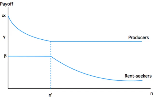
Assume an economy where one can engage in one out of three economic activities. First, say that a person can produce a good for the market, at the output of α. Second, the person can produce a subsistence good, at the output of γ<α. This good cannot be subjected to rent-seeking behavior, that is, it cannot be stolen or confiscated. However, that is not the case for the market output, which can be subjected to rent-seeking behavior. Further on, the third activity that a person can en-gage in is rent-seeking. It is denoted by β and it is the maximum amount at which he can produce. The overall return from production (including rent-seeking) will fall under the circumstances of an increase in rent-seeking activities.

The ratio of people engaging in market production and rent-seeking activities are denoted by n, and the income per capita by y. The equilibrium in this economy is established by the populations ac-cumulated engagements in either production of a good (α), subsistence production (γ<α) or rent-seeking (β). Therefore the allocation of labor will depend upon α, γ, and β.

In Case 1, β<γ, which correspond to figure 2. Under these circumstances property rights are well preserved and the society does not suffer from any corruption. The return for producers are higher than for seekers, additionally the return for subsistence producers are also higher than for rent-seekers. As we assume that individuals want to maximize their own output, under this situation each individual will produce goods and there are no subsistence producers or rent-seekers. The ra-tio of people engaging in rent-seeking activities is, n=0, and the return for rent-seekers is diminish-ing. However, n changes, let say n>0, the market production can be described by α-nβ (diminish-ing).

We assume the Gini coefficient to be zero. No corruption and well preserved property rights lead to the highest possible output (per capita), denoted by α.

Figure 2. Payoff to production and rent-seeking, β<γ

(15)

In Case 2 correspond to figure 3 where, β>α. Property rights are poorly preserved and therefore

due to the greater return for rent-seekers, people rather engage in rent-seeking activities than any-thing else. This is an extreme corrupt society. Figure 3 shows that there can only be one equilibri-um, at the point where the return from production has gone down to γ and that it is equal to the output from rent-seekers. This is when rent-seekers are crowding themselves out i.e., 𝛾 =(!!!_! , which in equilibrium is 𝑛!!=(∝!!)

! , given that n’’ >n’. In equilibrium all individuals’ income is the same as subsistence production γ, hence, the equilibrium is not where the market productivity is, at α2_.

The number of rent-seekers will increase over time and accordingly the number of producers will decrease, i.e. α-nβ=γ. As the number of individuals interacting in rent-seeking activities increase, the market output will decrease. The gini coefficient has a likelihood of being high. As higher Gini coefficient as closer to being completely equal.

Figure 3. Payoff to production and rent-seeking, β> α

Source: Murphy et al., 1993

In Case 3, γ <β<α. This last case we refer to an intermediate level of corruption which consist of

three equilibria as shown in figure 4. (a) The first equilibrium refers back to Case 1 where all people chose to produce in accordance with output α. (b) Second equilibrium comes from Case 2, where people chose among production (α), subsistence production (β), and rent-seeking activities (γ). This is encountered under the circumstances where income per capita is pushed down to γ, and equilib-rium based upon 𝑛 = ∝_!− 1. (c) The third equilibrium, where people either engage in market pro-duction or rent-seeking. The output is denoted by β. Observe that in this equilibrium there is no people engaging in subsistence production. The equilibrium is based upon α-βn=β, or n’’’= (∝!!)_! given that n’’’<n’. This occurs since new entries of rent seekers will force the return of the produc-ers on the market down to the same return as the rent-seekproduc-ers, and that is before any initiated crowding out. However, this last equilibrium is not stable, nor desirable as it push n beyond n’’’. Consequently, it implies a rising return to rent-seekers. Therefore there is only two stable equilibria, one where n=0 and another where n=n’’. In accordance with the former, less people will engage in rent-seeking activities than what is shown in case 2. Additionally the income level β is higher than in case 2, but still lower than case 1.

Concluding case 3, one can see that the variation in income will vary more than in case 1, however, not as much as in case 2. Countries which have a low corruption level will have a lower level of

(16)

in-come variation than countries with an intermediate or high level of corruption. The gini coefficient is higher than in case 1 but not as high as in case 2.

Figure 4. Payoffs to production and rent-seeking, γ<β<α

Source: Murphy et al., 1993

The empirical implications of the modified model we find that the best situation is case 1, where property rights are well preserved and no existing corruption. This is under the conditions of β placed below γ. It will lead to the highest possible per capita output, denoted by α. Anti-corruption beliefs, i.e. legal system or cultural impacts may also affect an important role (North, 1981).

Our hypothesis states:

 Property rights and corruption are negatively correlated

 A high level of corruption imply high income inequality

 The correlation between corruption and income inequality is negative

 Corruption should also have a negative correlation with income level

(17)

4 Data

The data have been constructed from several sources to compile a suitable dataset3_{. The dataset}

in-cludes 99 countries. The countries were not chosen by any random selection. We simply used all countries that had sufficient data both for the Gini coefficient and the corruption index. Countries included in the dataset can be found in Appendix 1. The variables4_{were collected from several}

dif-ferent sources as currently there is no single provider of all variables required.

Collecting accurate and qualitative data is found to be fairly difficult since corruption is illegal and its operations are mostly hidden as earlier discussed. Thereto there are no unified or general known method used by institutions. Historically one have been using indices as a method to measure cor-ruption in empirical studies (Dahlström, 2009). We use the corcor-ruption perception index (CPI), which is provided and accumulated by Transparency International. It is the far broadest index avail-able and it is matching our intentions with this paper as we are only interested in the percieived lev-el of corruption in a country. We are not targeting any specific form or measure of corruption. The CPI index currently contains data from 180 countries and has been recorded since 1995. The CPI rank countries from 0 (most corrupt) to 10 (least corrupt). For the sake of simplicity the index has been inverted, so now 10 indicates higher level of corruption.5

The Gini index is as explained in section 2 and it is the area between the line of equality and the Lo-renz curve. Indices for income inequality can be accumulated from different metrics. This paper us-es the Gini index, which is the most common metrics for income inequality. The Gini index fits our model best as we are computing for regressions in a cross-country sample. Gini coefficients are ac-cessed from the World Income Inequality Database 2 (WIID2), which is collected by UNU-Wider, United Nations University. The World Institute for Development Economic Research have updat-ed and checkupdat-ed the WIID1, which is a newer version of Deininger & Squire database from the World Bank. Deininger & Squire is otherwise a source that can be commonly seen in many other works. WIID2 also contain more measuring points and the fact that it is the world’s largest data-base of Gini coefficients makes it an appropriate source.6

The regressions and the empirical analysis is based upon a balanced dataset including averaged vari-ables between the years 2002 and 2006. Notice that we have only been using avareges. We sought to use as recent data as possible without abandoning a relatively good sample size. Most countries have complete variables, however, some years have missing gini coefficients. This will not represent any significant problem as the Gini coefficient merely face any radical changes over the time span of 5 years. The five-year average is used to eliminate any short-run variations and thus the variables will give a more universal representation of the genuine relationship.

3_{CPI was collection directly from TI, GINI was collection from WIID2 and the Legal Origin information}

was collection from La Parta (2000).

4_{Corruption Perception Index, Gini Coefficient, Countries Legal Origin}

5_{The CPI is inverted following Mauro (1995) and Li et al (2000). Ignoring the transformation of the}

corrupt-ion measure would make the comparison of graphs more difficult. See appendix 1.

(18)

Table 1. Descriptive Statistics of Gini Coefficient and Corruption Index

N Minimum Maximum Mean Std. Deviation

CPI 99 .34 8.46 5.7099 2.33705

GINI 99 23.98 57.90 38.7977 9.05152

Valid N (listwise) 99

Figure 5. A scatter plot describing the correlation between corruption and income inequali-ty. This figure covers average data for the years 2002 to 2006 for each country.

Source: Authors own production

Figure 5 shows that plotting the average gini against the average corruption index. The Gini coeffi-cient is positively correlated with Corruption. Implying that if corruption increases so will the gini coefficient.

Plotting the variables in figure 5 gives an indication of heteroscedasticity. However the visual ap-proach by simply revieving the scattered plot or the histogram of our dependent variable the gini coefficient will not statistically prove heteroscedasticity. Therefore, in appendix 5 we have present-ed the full testing of heteroscpresent-edasticity showing that we can reject the null hypothis of homoscpresent-edac- homoscedac-ity, hence heteroscedasiticity exists.

(19)

4.1 Model

When looking at how corruption affects income inequality we use these following linear regression model. Using a Weighted Least Squares regression method. One of the reasons of showing the WLS regression model would be the heteroscedasity previously discussed.

𝐺𝐼𝑁𝐼!= 𝛽!𝐶𝑃𝐼!+ 𝛽!𝐷!"#$%&$'(+ 𝛽!𝐷!"#$%&!+ 𝛽!𝐷!"#$%!+ 𝛽!𝐷!"#$%&+ 𝛽!𝐷!"#$%&+ 𝜀! (1)

𝐺𝐼𝑁𝐼_!= 𝛽_!+ 𝛽_!𝐶𝑃𝐼_!+ 𝜀_! (2)

These models hold the income inequality (GINI) as the depended variable and Corruption index (CPI) as independent variable. Following our purpose we look for patterns depending on different groupings based upon legal system. Model 1 include dummy variables following the La Porta grouping, identifying legal systems.

Y : An average of each countries gini coefficient over 2002-2006

X1 : An average of each countries corruption perception index over 2002-2006 DSocialist : Dummy indicating if a country’s legal system is identified as Socialist DEnglish : Dummy indicating if a country’s legal system is identified as English DFrench : Dummy indicating if a country’s legal system is identified as French DGerman : Dummy indicating if a country’s legal system is identified as German DScandinavia: Dummy indicating if a country’s legal system is identified as Scandinavia

4.1.1 WLS vs OLS

The ordinary least squares (OLS) estimator is the best method to use if random errors in a linear regression model are having the same variances, that is, the standard deviation of the error term is contant (Shao, 1990). However, many regressions shows that the opposite, as in our case, that the size of the variances of random errors are different from each other. This imply that the result will not be optimized and the OLS model is not the appropriate approach in selection of model. Instead of the OLS regression estimator one can use a WLS regression model. The WLS has some advantages. One of the greatest advantages is that the model fits small data sets (Shao, 1990) and the WLS regression also can be a good measure when the variances in the random errors are not the same (Carrol, 1982).

Furthermore we continued with the WLS method as it gave us both better R2_{and a lower S}_e_.

4.1.2 The WLS regression model

In a linear regression one of the common assumptions is that each data point gives accurate infor-mation of their respective part in the total variation. That is, the standard deviation of the error term is constant. Undoubtedly this will not always be the case. In line with the former, one cannot always assume that all data points should be treated equally. By analysing Figure 5, the scatter plot of the gini coefficient and the corruption index, we can see that we have some distant data points, where some countries have performed indifferent with the hypothosis, i.e. low gini but high corrup-tion or the other way around (e.g. Chile or Slovakia).

(20)

In our WLS regression we use corruption as a weighted variable and can produce a more efficient estimation of the parameters. The observations are weighted relatively to the weight of the other observations.

With a WLS regression we produced a good estimate for the relationship of corruption and income inequality. However, the WLS regression is not all pros, there are some cons which are worth men-tioning. First, the WLS theory assumes that the weights are known, which obviously almost never I the case. Therefore one estimates the weights in a WLS regression . The affects of using estimated weights instead of real weights is argued to have minor impacts on the actual regression interpreta-tion. Secondly, outliners still have an impact on the regression result as in any other least squares regression, but to overlook the WLS as an appropriate method would result in an analysis with low-er quality and less significance.

(21)

5 Results

Our thesis is based upon cross section data constructed by 99 countries. These 99 countries were the only countries that had sufficient data presented between the years 2002 and 2006 on both the measures of corruption and income inequality. A full review of the dataset can be found in Appen-dix 1.

The legal origin of each group is divided as follows: English (19), Socialist (32), French (38), Scan-dinavian (5), and German (5) (a full specification can be found in Appendix 2). The countries are divded into these sub groups depending upon their legal system.

The tables in Appendix 3 shows the full results for the WLS regression model (1) including dum-mies depending upon legal origin. The R2_{reported in the regression is .500 which is reasonably}

good for only including one independent variable. Consequently about 50% of the movements of corruption explains the affects on income inequality, holding all other unknown variable the same. Comparing the regression results from the WLS regression with dummies and the WLS regression without dummies we can see that our results are stronger in the case with dummies included. The below coefficient tables shows the results including dummy variables:

The dependent variable is GINI

Table 2. Regression of income distribution and corruption with legal origin as dummies.

In the regression we do achive significant results on the CPI variable. However, none of the dum-my variables do meet signifanct values for the 5% nor the 10% confidence interval. Also notice that the German dummy variables was excluded in the regression results as the high correlation between the dummy variables.

We recognize that we may have some endogeneity concerns between our variables. However as we are only including two variables and dummies we chose not to test the effectiveness of the endoge-neity.

It is typically safe to assume that the errors are uncorrelated as we use cross-section data, however the variances may not be constant over all individuals.

Other omitted variables that one can include in the reasoning would be countries’ differences in Coefficients

Unstandardized Coefficients Standardized Coefficients

t Sig. B Std. Error Beta Std. Error

(Constant) _26,088 _2,647

_9,857 _,000 CPI 2,060 ,340 ,632 ,104 6,058 ,000 ENGLISH 2,652 3,026 ,117 ,133 ,876 ,383 SOCIALIST -3,915 3,238 -,185 ,153 -1,209 ,230 FRENCH 4,127 2,987 ,215 ,155 1,382 ,170 SCANDI -,823 3,169 -,031 ,119 -,260 ,796

(22)

both GPD and Education Level. Both GDP and Education level has in previous research shown significant results on Income Inequalities. (Barro, 2000). However, we are limiting our research to our purpose and choose not to broaden the scope too extensively. Neverthereless, we recognize that GPD and Education level do probably have a great impact on income inequalities among countries.

We have also not allowed any discussions nor reasoning from the pruposed effects from different religion.

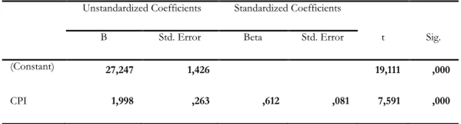
Moreover, the coefficient table below shows our results without any dummy variables: Coefficients

(Constant) _27,247 _1,426

_19,111 _,000

CPI 1,998 ,263 ,612 ,081 7,591 ,000

The dependent variable is GINI

Table 3. Regression of income distribution and corruption without any dummies.

Our model remains significant with or without dummies. However the WLS regression encompass-ing dummies dependencompass-ing upon legal origin shows better results both in R2_{and Std. Error of the}

Es-timate. The dummies were created to see how it would affect the movement from corruption on income inecquality and see if the data set could fit the model better. Consequently our results shows that corruption is affecting income inequalities negatively.

In appendix 6 we provide single regressions on each one of the dummy variables against the gini coefficient. All legal origins are independently showing significant results between CPI and gini. Additionally appendix 7 includes regressions on the complete dataset but without CPI to show the relation of the dummies versus GINI.

(23)

6 Conclusion

Corruption is generally known for its adverse affects on economic growth. While in this thesis we have put some light on corruptions’ adverse affects on income inequality. By using a framework which in its original form was first presented by Murphy et al. (1991, 1993), and then adjusted by Li et al. we have showed how a countries’ legal origin can have an impact. Data on both corruption and income inequality has become much larger and better every year, and it has allowed us to in-clude more than twice the countries’ than e.g. Li et al.

We find that with our regressions and analysis a country with high corruption also has high income inequality. Additionally we added the legal origin of countries in order to compare significance in the correlation between corruption and income inequality.

Additionally the Appendix 6 shows that all legal systems are individually representing a significant result between the dependent variable income inequality and corruption.

We belive that with a larger sample size the evidence becomes more reliable and the probability of any error will decrease.

Our contribution has been towards the patterns that one can project from our regressions. Valuable information and conclusions can be drawn from both the regression model with and without dummies. Additionally regressions on each legal origin group has been composed to show signifi-cant results on each one of the groups.

Suggestions for further research that could be of use and give even better results is to continue us-ing new and greater datasets as they become available. The difficulties with measurus-ing and definus-ing corruption will sustain however without trying to change either the method of measuring or the definition one can compare newer research with previous for a greater understanding. We only reach a dataset of 99 countries, hopefully more data will become more accessible and a greater data sets can be constructed. As greater dataset are conducted accuretly one can start looking at cross regional regressions for each region depending upon legal origin and possibly achive greater signifi-cance in each group of countries.

(24)

References

Acemoglu, D., Johnson, S, Robinson, J.A., 2001. The Colonial Origins of Comparative Develop-ment: An Empirical Investigation, The American economic review, Vol. 91, No. 5, pp.1369-1401 Ackermann, S., R., 1999. Corruption and Government: Causes, Consequences and reform.

Cam-bridge University Press.

Atkinson AB, 1970, On the measurement of inequality., Journal of Economic Theory, 2, 244-263 Banfield, Edward. 1958. The Moral Basis of a Backward Society. New York: Free Press.

Barro, Robert J. 2000. Inequality and Growth in a Panel of Countries. Journal of Economic Growth, 5: 5-32. pp. 24

Carroll, John S., Jolene Galegher, and Richard L. Wiener. 1982. Dimensional and Categorical At-tributions in Expert Parole Decisions, Basic and Apploed Social Psychology. pp. 187.

Dahlström, T. 2009, Causes of corruption, JIBS Dissertation Series No. 059

Daniel Kaufmann, 1997, Corruption: The facts, Foreign Policy, No. 107 (Summer), pp. 114-31 Daniel Treisman, 2000. The Causes of Corruption: A Cross-national Study. Journal of Public

Econom-ics 76, pp. 399-457

Gupta, S., Davoodi, H., Alonso-Terme, R., 1998, Does corruption affect income inequality and poverty? Working Paper of the International Monetary Fund WP/98/76.

Hoover, E. M. Jr., The Measurement of Industrial Localization, Review of Economic and Statistics, 1936, Vol. 18, 162-171

Jakob Svensson, Summer 2005, Eight questions about corruption. Journal of Economic Perspective, Volume 19, Number 3. P. 19-42

James D Gwartney, Randall G. Holcombe & Robert A. Lawson, 2006. “Institutions and the Impact of Investments on Growth”. Kyklos, Vol. 59 – 2006 – No. 2, p.255 – 273.

Kaufmann, Daniel, Aart Kraay, and Pablo Zoido-Lobaton. 1999a. Aggregating Governance Indica-tors. Policy Research, Working Paper 2195, World Bank

Kaufmann, Kraay and Mastruzzi, 2003. Governance Matters III: Governance Indicators for 1996-2002, World Bank

Landes, David. 1998. The Wealth and Poverty of Nations. New York: W. W. Norton.

La Porta, Rafael, Florencio Lopez-de-Silanes, A. Schleifer and R. Vishny, 2000, The Quality of Government. Journal of Economics and Organization, 15:1. 222-279

Leff, N., 1964, Economic development through bureaucratic corruption. American Behavioral Scientist 8, 6-14.

Li, H., Xu, C., Zou, H., 2000, Corruption, income distribution, and growth. Economics and Politics Vol. 12, 155-181

(25)

Lorenz Curves and the Gini Coefficient from the Wolfram Demonstrations Project. Retrived on 2013-06-07, Available at http://demonstrations.wolfram.com/ LorenzCurvesAndTheGiniCoefficient Lui, F. T., 1985, An equilibrium queuing model of bribery. Journal of Political Economy 93, 760-781. Mauro, P., 1995, Corruption and growth. Quarterly Journal of Economics 110, 681-712.

―,1996. The effects of Corruption on Growth, Investments, and Government Expenditure. Inter-national Monetary fund , Working paper/96/98

―, 1997. Why worry about Corruption, Economic issues, 6, International Monetary Fund, Washington D.C.

―, 1998, Corruption and the Composition of Government Expenditure, Journal of Public Economics, 263-269

―, 1998, Corruption: Causes, Consequences, and Agenda for Further Research. Finance and develop-ment Vol 35; No 1, 11-14

Murphy, K., A. Shleifer, and R. Vishny, 1991, The allocation of talent: implication for growth. Querterly Journal of Economics 105, 503-530

―, ―, and ―, 1993, Why is rent-seeking so costly to growth? American Economic Review, May, 409-414

North, Douglass, C., 1991, Institutions, Journal of Economic Perspective, vol. 5; No.1, pp. 97-112 Putnam, Robert. 1993. Making Democracy Work: Civic Traditions in Modern Italy. Princeton:

Princeton University Press.

Scott J.C 1972, p.66, Comparative Political Corruption, Prentice-Hall, Englewood Cliffs, New Jersey. Shao, J. 1990. A winter road surface temperature model with comparison to others. Unpublished PhD

thesis, University of Birmingham, UK.

Theil, H., 1967, Economics and Information Theory, North Holland Publishing Company, Amsterdam 1967

The world bank., 2009, Poverty analysis. Retrived on 2009-10-09, Available at: http://go.worldbank.org/77LE4ON4V0

Transparency International, 2009. Corruption threatens Global Economic Recovery, greatly chal-lenges countries in Conflict, Berlin 17 November, 2009. (Accessed 2010-01-13) Available at:

http://transparency.org/news_room/latest_news/press_releases /2009/2009_11_17_cpi2009_en

Van Rijckeghem and Weder, 1997, Corruption and the Rate of Temptation: Do low wages in the Civil Service Cause Corruption?, International Monetary Fund, Working Paper/97/73

Weber, Max. 1958. The Protestant Ethic and the Spirit of Capitalism. New York: Charles Scribner’s Sons.

World Bank, 1997, World Development Report: The State in a Changing World, New York: Oxford University Press

(26)

Appendix 1 Countries included in the dataset (99 countries).

Albania Dominica Kyrgyzstan Portugal

Argentina Ecuador Lao People's Democ Romania

Armenia Egypt Latvia Russian Federation

Australia El Salvador Lithuania Serbia & Montenegro

Austria Estonia Luxembourg Sierra Leone

Azerbaijan Finland Macedonia Slovakia

Bangladesh France Malawi Slovenia

Belarus Georgia Malaysia Spain

Belgium Germany Malta Sri Lanka

Benin Greece Mexico Sweden

Bolivia Guatemala Moldova Switzerland

Bosnia and Herzego Guinea Mongolia Tajikistan

Brazil Honduras Mozambique Thailand

Bulgaria Hungary Nepal Turkey

Burkina Faso Iceland Netherlands Uganda

Cambodia India New Zealand Ukraine

Chile Indonesia Nicaragua United Kingdom

China Iran, Islamic Repu Nigeria United States

Colombia Iraq Norway Uruguay

Costa Rica Ireland Pakistan Uzbekistan

Côte d'Ivoire Italy Panama Venezuela

Croatia Jamaica Paraguay Viet Nam

Cyprus Japan Peru Yemen

Czech Republic Kazakhstan Philippines Zambia

(27)

Appendix 2 This appendix outlines the groupings depending upon legal origin.

ENGLISH Australia Bangladesh Cyprus

India Ireland Jamaica Malawi

Malaysia Nepal New Zealand Nigeria

Pakistan Sierra Leone Sri Lanka Thailand

Uganda United Kingdom United States Zambia

SOCIALIST Albania Armenia Argentina

Azerbaijan Belarus Bosnia and Herzegovina Bulgaria

Cambodia China Croatia Czech Republic

Estonia Georgia Hungary Kazakhstan

Kyrgyzstan Laos Latvia Lithuania

Macedonia Moldova Mongolia Poland

Romania Russian Federation Slovakia Slovenia

Tajikistan Ukraine Uzbekistan Viet Nan

FRENCH Belgium Benin Bolivia

Brazil Burkina Faso Chile Colombia

Costa Rica Côte d'Ivoire Ecuador Egypt

El Salvador France Greece Guatemala

Guinea Honduras Indonesia Iran, Islamic Republic

Iraq Italy Luxembourg Malta

Mexico Mozambique Netherlands Nicaragua

Panama Paraguay Peru Philippines

Portugal Serbia & Montenegro Spain Turkey

Uruguay Venezuela Yemen

SCANDINAVIAN Denmark Finland Iceland

Norway Sweden

GERMAN Austria Germany Japan

(28)

Appendix 3

WLS regression model (1) including dummies depending upon legal origin.

Model Summary

Multiple R ,707

R Square ,500

Adjusted R Square ,472

Std. Error of the

Esti-mate 4,701

Log-likelihood Function

Value -326,122

ANOVA

Sum of Squares df Mean Square F Sig.

Regression 2028,989 5 405,798 18,365 ,000

Residual _2032,898 ₉₂ _22,097

Total _4061,887 ₉₇

Coefficients

(Constant) _26,088 _2,647

_9,857 _,000 CPI 2,060 ,340 ,632 ,104 6,058 ,000 ENGLISH 2,652 3,026 ,117 ,133 ,876 ,383 SOCIALIST -3,915 3,238 -,185 ,153 -1,209 ,230 FRENCH 4,127 2,987 ,215 ,155 1,382 ,170 SCANDI -,823 3,169 -,031 ,119 -,260 ,796

(29)

Appendix 4

WLS Regressions results without any dummies.