It’s a match?
MASTER THESIS WITHIN: Economics NUMBER OF CREDITS: 30 ECTS
PROGRAMME OF STUDY: Economic Analysis AUTHOR: Emil Karlsson
TUTORS: Charlotta Mellander & Orsa Kekezi JÖNKÖPING June 2019
A comparison of the aggregated job-matching efficiency
in urban and rural regions in Sweden
i
Master Thesis in Economics
Title: It’s a match? – A comparison of the aggregated job-matching efficiency in ur-ban and rural regions in Sweden
Authors: Emil Karlsson
Tutors: Charlotta Mellander & Orsa Kekezi Date: 2019-06-10
Key terms: Job-matching efficiency, Beveridge curve, Labor market, Urban, Rural, Sweden
Abstract
The purpose of this thesis is to examine if there is a difference between Swedish urban and rural regions in terms of job-matching efficiency. The thesis employs the Beveridge curve with un-employment rate as the dependent variable as a framework and a longitudinal dataset covering 60 regions and the period 1998-2015. Two aspects of the job-matching efficiency are consid-ered; the determinants of unemployment and the temporal changes in the job-matching effi-ciency. Considering the determinants of unemployment, some differences between urban and rural regions are detected. The results indicate that the mean age of a region’s population is negatively related to the unemployment rate while the share of women in the labor force is positively related in both types of regions. According to the Beveridge curve, this implies that the job-matching efficiency increases with a higher mean age while a higher share of women in the labor force decreases the matching efficiency. However, both variables are significantly stronger related to the unemployment rate in urban regions. Education is found to be positively associated with unemployment rate in urban regions while insignificant in rural ones. Lastly, no major difference between the two types of regions regarding the changes or position of the Beveridge curve are found. This implies that the job-matching efficiency is similar and change simultaneously in both urban and rural regions.
ii
Table of Contents
1. Introduction ... 1
2. Background ... 5
2.1 Theoretical framework ... 5
2.2 What affects the job-matching efficiency? ... 7
2.3 Previous findings of changes in job-matching efficiency ... 10
3. Methodology ... 12
3.1 Empirical model ... 12 3.2 Data ... 13 3.2.1 Variables ... 14 3.2.2 Descriptive statistics... 16 3.2.3 Correlation analysis ... 17 3.3 Econometric model ... 184. Results ... 19
4.1 Determinants of job-matching efficiency... 19
4.2 Movement of the curve ... 22
4.3 Robustness checks ... 25
5. Discussions ... 26
5.1 Discussion on the determinants of unemployment ... 26
5.2 Discussion on the movement of the curve ... 29
5.3 Limitations ... 30
6. Conclusion ... 33
iii
Figures
Figure 1 – The Beveridge curve ... 2
Figure 2 – Change in the intercept of Beveridge curve ... 24
Tables
Table 1 – Description of variables ... 16Table 2 – Descriptive statistics FA-regions 1998–2015 ... 17
Table 3 – Correlation matrix ... 17
Table 4 – Dependent variable: Unemployment rate ... 20
Table 5 – Dependent variable: Unemployment rate ... 23
Table 6 – Movements of the Beveridge curve ... 24
Appendices
Appendix 1. – FA-regions ... 38Appendix 2. – Descriptive statistics ... 40
Appendix 3. – Regressions with interaction terms ... 41
1
1. Introduction
A vast majority of the Swedish population lives today in urban areas (SCB, 2015) and the three largest regions account for more than 50 percent of the total population in Sweden in 2018. Living in an urban region can have many advantages. For example, urban regions have a greater and more diverse supply of amenities (Glaeser, 2011). Furthermore, ag-glomeration gives rise to positive externalities, such as knowledge spillovers, which gen-erate a higher level of productivity (Glaeser, Kallal, Scheinkman & Shleifer, 1992). How-ever, while larger regions have experienced population growth, smaller regions have in-stead faced depopulation (Mellander, 2019). Such regions tend to face greater difficulties to stay attractive as people chose to move to larger regions. Just as amenities and positive externalities attract individuals to an urban region, do likewise a lack of such assets deter people to live in such areas and rural regions are losing inhabitants (SvD, 2018).
Related to regions’ attractiveness are the labor markets and unemployment is a problem which exist in the whole country. On a national level, 321 200 individuals were unem-ployed in December 2018 and 97 800 had been without work for more than six months (SCB, 2019). This correspond to an unemployment rate of 6.2 percent. The cost of unem-ployment is large, where 12.4 billion SEK was paid for unemunem-ployment benefit (a-kassa) and the cost for activity support and personal development (aktivitetsstöd och
utvecklings-ersättning) was 13.4 billion SEK in 2016 (Akademikernas a-kassa, 2018). Furthermore,
five billion SEK is paid in social welfare (försörjningsstöd) which are due to unemploy-ment. However, none of these costs measure the opportunity cost of being unemployed. Except for the direct cost, unemployment and vacancies also result in losses in the tax base for the government and lower the production capacity. Given the costs of both vacancies and unemployment, it is important to know how the job-matching efficiency can be im-proved. Nevertheless, the job-matching efficiency might not be the same in different re-gions and actions aimed to improve the effectiveness might work in some types of rere-gions but not in others (Coles & Smith, 1996).
This thesis aims to examine what is known in the literature as job-matching efficiency by employing the Beveridge curve as a conceptual framework. The curve, depicted in Figure 1, shows the relationship between unemployment and job vacancies and is a common framework for studying how effective the job-matching process is in a country or region
2
(Kosfeld, Dreger & Eckey, 2008). According to the curve there is a negative convex rela-tionship between the two factors.
With a high level of job vacancy (i.e., where the demand for workers is high), unemploy-ment tends to be low since finding a job is relatively easy. High unemployunemploy-ment, on the other hand, is usually correlated with fewer vacancies, which makes it harder to find a job. The job-matching process is said to be less effective the further away the curve is from the origin. Movements along the curve are typically ascribed to the current business cycle and shifts are due to structural changes which affect the individuals’ ability to find a matching job (e.g., human capital, age, population density etc. (Wall & Zoega, 2002)). As such, if the unemployment rate increases for a given rate of vacancies, the curve shifts out and the job-matching becomes less efficient. Job-matching should in this context be understood as how well the aggregated labor force characteristics match the characteristics demanded by the firms. If both the demand and supply were completely homogenous, the Beveridge curve would be at the origin and there would be no mismatch.
The employed longitudinal dataset includes information for the years 1998-2015 for func-tional analysis regions (FA-regions1) on vacancy, unemployment and several control var-iables which are said to be associated with shifts of the curve. To capture the potential urban/rural difference, the regions will be classified according to the three regions-types which the Swedish Agency for Growth Policy Analysis, Growth Policy, has defined
1 FA-regions define functional labor markets regions and are based on commute patterns across
municipali-ties borders.
u
v
3
(Tillväxtanalys, 2011). Based on what is previous stated, the research question is formal-ized as: is there a difference in the job-matching efficiency between urban and rural
re-gions in Sweden? Two steps will be taken in order to answer this question. The first step
follows the approach employed by Bouvet (2012) and includes a regression where the un-employment rate is dependent on the vacancy rate and several controls variables. The pur-pose of this this stage is to examine which factors influence the unemployment in the dif-ferent types of regions and in Sweden as a whole. The next step is to examine the move-ment of the curve, following Börsch-Supan (1991) and Wall and Zoega’s (2002) method-ologies, which regress unemployment rate on vacancy rate and control variables together with year dummies. This makes it possible to observe in which years the Beveridge curve has shifted direction and to see if the national movement of the curve corresponds to the regionals.
While previous articles have examined the job-matching efficiency from a regional aspect (Börsch-Supan, 1991; Bonthuis, Jarvis & Vanhala, 2013; Bouvet, 2012; Coles & Smith, 1996; Eklund, Karlsson & Pettersson, 2015; Kosfeld et al., 2008; Valletta, 2005; Wall & Zoega, 2002), this thesis differentiate itself by considering the potential difference between urban and rural FA-regions. According to Duranton and Puga (2003), there are reasons to believe that urban regions have a higher matching efficiency. They argue that in urban regions there are more agents working on matching unemployed and vacancies with each other. As such, both the numbers and quality of the matches increase. Similar thoughts have also been expressed by Coles and Smith (1996), in where the population density im-proves the job-matching efficiency.
The results in this thesis indicate that there are some differences between urban and rural regions in terms of the determinants of the unemployment rate. For both types of regions, the mean age of a region’s population is negatively associated to the unemployment rate while the share of women in the labor force is positively related. This implies, according to the theory, that the job-matching efficiency increases with a higher mean population age while the efficiency decreases with a higher share of women. However, both variables are significantly stronger related to the unemployment rate in urban regions. In addition, there is no significant difference in the position of the Beveridge curve between urban and rural regions, which indicates that the job-matching efficiency is similar in both types of regions. Lastly, the movement of the curve seems to correlate between urban and rural regions. This
4
suggest that when the job-matching efficiency increases in one type of region, it often increases in the other type of region as well.
This paper is organized as follow: first, in section 2 will the background on the Beveridge curve be presented together with the empirical findings of previous research. This is fol-lowed by section 3, where the econometric models will be introduced together with a de-scription of the data. The results follow in section 4 and are discussed in section 5. Section 6 concludes the thesis.
5
2. Background
This section will give a background on the topic of job-matching efficiency. It starts with the theoretical framework. This is followed with an outline over some of the factors which are related to the job-matching efficiency. Lastly, an overview of how the job-matching efficiency have developed in different countries will be presented.
2.1 Theoretical framework
The Beveridge curve appeared originally in Dow and Dicks-Mireaux’s (1958) analysis of the British labor market. They describe a curve which are convex towards the origin and shows the relationship between vacancies and unemployment. The convexity is due to that there will always be some level of unemployment, even when the demand for labor is high (i.e., high number of vacancies). The same is true for vacancies as there will always be some unfilled demand for labor. As such, there is a decreasing sensitivity to both supply and demand, which give rise to the curvature of the relationship.
The curve has since Dow and Dicks-Mireaux (1958) been employed as a framework for examining job-matching efficiency in many studies (see e.g., Blanchard and Diamond (1989), Börsch-Supan (1991), Petrongolo and Pissarides (2001), Wall and Zoega (2002), Kosfeld et al. (2007), Bouvet (2012) and Eklund et al. (2015)). However, for long time the curve was neglected in the research which was noted by Blanchard and Diamond in 1989. They argued that the Beveridge curve has “very much played second fiddle” (p.1) in rela-tion to another labor market curve, the Philips curve, which shows the relarela-tionship between unemployment and inflation. The neglection of the Beveridge curve is also noted by Eklund et al. (2015), which find it surprising that the framework has not been applied in more studies. However, Blanchard and Diamond’s (1989) article might have helped to promote the utilization of the Beveridge curve, as the years after it was published have shown a renew interest in the curve’s usefulness. Furthermore, Eklund et al. (2015) state that employing the Beveridge curve as a theory allows researchers to better understand job-matching efficiency and which factors that influence the dynamics of the labor market. The starting point for deriving the Beveridge curve is a standard aggregated matching func-tion
𝑀 = 𝑀(𝑈, 𝑉) (1)
where the number of matches M is a function of unemployment U and vacancies V. In-creasing either U, V or both would increase the numbers of matches occurring. The survey
6
made by Petrongolo and Pissarides (2001) on previous usage of the Beveridge curve have shown that equation 1 is usually expressed as a Cobb-Douglas function. Therefore, equa-tion 1 can be transformed into
𝑀 = 𝐴𝑈𝛾𝑉1−𝛾 (2)
where A is the matching efficiency which changes the position of the Beveridge curve (see e.g., Wall and Zoega (2002), Kosfeld et al. (2007) and Bouvet (2012)). Petrongolo and Pissarides (2001) have find that previous research indicates a constant return to scale where 0< 𝛾 <1. Some articles (e.g., Coles and Smith (1996), Dur (1999), Aranki and Löf (2008) and to some extent also Eklund et al. (2015)) have chosen to stop here and estimate equa-tion 2 in their analyses of the matching process. To arrive at the final equaequa-tion for the Beveridge curve, more derivations are however needed. The implicit form of equation 2 is obtain by dividing all factors by the labor force, which yields:2
𝑚 = 𝑎𝑢𝛾𝑣1−𝛾 (3)
When the labor market is in a steady state, the number of separations s (e.g., when an employer lays off employees) are equal the number of matches m. Hence,
𝑠 = 𝑎𝑢𝛾𝑣1−𝛾 (4)
Finally, Bouvet (2012) have shown that, with s fixed, equation 3 can be written as
𝑢 = ( 𝑠
𝑎𝑣1−𝛾) 1
𝛾 (5)
which depicts an inverse relationship between the unemployment rate and the vacancy rate when the labor market is in equilibrium. Previous literature has found that the negative relationship between unemployment and vacancies holds empirically (Bonthuis et al., 2013; Bouvet, 2012; Börsch-Supan, 1991; Eklund et al., 2015; Kosfeld et al., 2007; Val-letta, 2005; Wall & Zoega, 2002). The main interest is thus not the connection between these two variables, but of the matching efficiency parameter A and the factors which can be included in the parameter.
2 Some papers have chosen to divide A with the labor force, e.g., Kosfeld et al. (2007). Others, for example
7
2.2 What affects the job-matching efficiency?
As previous mentioned, the matching efficiency parameter A changes the position of the Beveridge curve and is related to structural changes. A more efficient job-matching process shifts the curve towards the origin, indicating that both vacancies and unemployment will be lower. On the other hand, if the efficiency of the job-matching process decreases, the curve shifts out from the origin and both variables would increase. Blanchard and Diamond (1989) argue that the matching efficiency parameter introduced to the model add the nota-tion of heterogeneity among the unemployed and the new jobs available. As such, the pa-rameter is included to capture the mismatch between the two main variables. If no mis-match occurred in the labor market, there would not be a need of a mis-matching function as it would be a direct match between unemployed and vacancies. Similarly, Dow and Dicks-Mireaux (1958) argues that vacancies and unemployment coexist since the labor offered by the unemployed differ from the labor demanded by the firms.
The literature has identified a number of factors which affect the job-matching efficiency. The matching efficiency parameter A can be decomposed into several components, where some of the more prominent will be discussed below. However, as A can be seen as a residual which capture all factors that are related to the job-matching efficiency, it is not feasible to measure all the factors which are included in the parameter.3
Education
Blanchard and Diamond (1989) state that the level of education is an aspect included in the matching efficiency parameter A. Similar, Petrongolo and Pissarides (2001) argue that mismatch is often thought of being a measure of the heterogeneity in skills, location and sectors. For example, if the skills offered by the unemployed do not correspond to the skills that the hiring firms require, there would be a large degree of mismatch and the Beveridge curve would shift out. However, examinations of the relationship between education and job-matching efficiency gives ambiguous results. Badinger and Url (1991) and Dur (1999) find that education is insignificant in both Austria and the Netherlands, respectively. Cole and Smith (1996) report on the other hand that an educated workforce significantly reduces the matching efficiency and a large share of firms within the manufacturing industry
3 One can view the matching efficiency parameter as akin to the residual in a production function a la Solow
8
improves it in the UK. According the Cole and Smith (1996), this could mean that manu-facturing jobs requires low-skilled workers where the matching process is simpler, while an educated workforce makes it harder for matches to occur. However, Bonthuis et al. (2013) find that a greater percentage of low-skilled workers increases the probability of mismatch in the euro area while the proportion of high-skilled workers is insignificant. In Sweden, Eklund et al. (2015) report a difference in the matching efficiency between low- and high-skilled workers. They find that the market for unskilled labor is affected to a greater extent of cyclical factors in relation to the educated workforce. The labor market for skilled workers also benefits when the share of the educated population increases in a region while on the other hand, unskilled labor is affected negatively of it.
Demographic characteristics
Several articles also point out the impact of other demographic characteristics of the labor pool as important for the job-matching efficiency, such as the sex and age composition (Bouvet, 2012; Börsch-Supan, 1991; Cole & Smith, 1996; Petrongolo & Pissarides, 2001; Samson; 1994; Wall & Zoega, 2002). Both Samson (1994) and Bouvet (2012) argue that women are less attached to their jobs which reduce the job-matching efficiency. Women could for example exhibit a lower level of attachment because of maternity or that they are relatively less qualified compare to men. In addition, Bouvet (2012) also argues that young people are less attached to their jobs. Both Samson (1994) and Bouvet (2012) find empir-ical support that women increase the unemployment rate and reduce the job-matching ef-ficiency. Bouvet (2012) further finds that younger people are associated with a higher un-employment rate. In common with Samson (1994) and Bouvet (2012), Börsch-Supan’s (1991) results indicate that a higher proportion of unemployed women shifts the Beveridge curve outwards.
Concerning the age composition, the results of Bonthuis et al. (2013) contradict Bouvet (2012) for young individuals. Bonthuis et al. (2013) argue instead that youngsters are less specialized and have less specifics skills, which both create lock-in effects, compared to more experienced individuals. As such, the duration of unemployment is shorter for young people. Furthermore, both Börsch-Supan (1991) and Badinger and Url (2002) find that age is insignificant.
9
Density
Coles and Smith (1996) point to the fact that it is not the sheer stock of unemployment and vacancies which gives raise to the matching process, but it is the population density. They argue that if the labor market was concentrated to a single region, more matches would occur, and the matching process would be more efficient.4 When controlling for the re-gional population density, Coles and Smith (1996) find that dispersion is significant and negatively related to the matching rate.
Similar thoughts have also been expressed by Aranki and Löf (2008) regarding the heter-ogeneity among regions. Aranki and Löf (2008) show that there is a significant variation in the job-matching efficiency in Swedish counties. Surprisingly, their analysis indicates that the three largest counties (i.e., Stockholm, Västra Götaland and Scania) have a relative low efficiency, while Jämtland county is the most efficient.5
Cyclical fluctuations
While business cycles are often associated with movement along the Beveridge curve and not usually included in the matching efficiency parameter (Wall & Zoega, 2002), some articles (Bouvet, 2012; Kosfeld et al. 2008) have chosen to include cyclical fluctuations in their estimations of the curve. Kosfeld et al. (2008) state that the conclusion regarding the job-matching efficiency based on the Beveridge curve could be “seriously biased” (p. 970) if shifts are not only caused by structural factors. Furthermore, Wall and Zoega (2002) acknowledge that if two regions move along their fixed Beveridge curve (perhaps due to cyclical fluctuations) but in opposite direction to one other, this will result in an outward shift of the aggregated curve.
Kosfeld et al.’s (2008) examination of the Beveridge curve shows that cyclical fluctuations are indeed significant for causing outwards shifts of the curve. In a similar fashion, Bouvet (2012) includes a measure of cyclical fluctuations as she argues that shifts of the curve are not solely due to structural factors. The results from Bouvet’s (2012) analysis indicate that
4 This is the reason why they argue that it is not reasonable to use time-series data which covers just one
aggregated region, such a nation.
5 For the sake of comparison, the counties of Stockholm, Västra Götaland and Scania belong to FA-regions
10
the cyclical fluctuations are significant but contradict the conclusion reached by Kosfeld et al. (2008) where cyclical fluctuations shift the curve outward.
2.3 Previous findings of changes in job-matching efficiency
In addition to which factors are related to the efficiency of the job-matching, previous ar-ticles have also been interested in examining when the shifts of the Beveridge curve actu-ally happen in time (Blanchard & Diamond, 1989; Bonthuis et al., 2013; Bouvet, 2012; Börsch-Supan, 1991; Eklund et al., 2015; Valletta, 2005; Wall & Zoega, 2002). As a start-ing point, such articles plot vacancies and unemployment and try to visually examine any movement of the curve. Bouvet (2012) has found that Belgium, Germany, the Netherlands, Spain and the UK were on stable curves from 1975-1985 and that the curves shifted out in subsequent years, indicating a less effective job-matching. Contradicting the results of Bouvet (2012) for Germany, Börsch-Supan (1991) finds that the curve has move outward three times in the period 1975-1984. Analysis on more recent data by Bonthuis et al. (2013) reveals that the job-matching efficiency has improved in Germany after the financial crisis 2008. However, both France and Italy have a less effective job-matching after the crisis, while the curve movement in Spain is inconclusive. For the US, Valletta (2005) reports that the Beveridge curve has exhibit an outward movement from the 1960’s to the mid-1980’s. Subsequently years have on the other hand seen an improvement in the job-match-ing efficiency.6 Eklund et al. (2015) have shown that the Swedish Beveridge curve has shifted outwards for the period 1981-2000. The following period that ended in 2014 started with a more efficient job-matching in the first half, which was succeed with an outward shift.
While scatterplots can serve as a good starting-point for the examination of the job-match-ing efficiency, such method is a rather blunt tool. Often is the relation between unemploy-ment and vacancies not a clear curve but is rather blurred, which leaves it to the researcher to semi-arbitrarily decide when a shift has occurred (Wall & Zoega, 2002). In addition, while scatterplots examinations are feasible to conduct when one examines a large set of countries or regions, it is not really practical.
6 As Valletta’s (2005) dataset cover the year 1960-2005, it is not possible to see the effect of the financial
11
To obtain more robust result, some articles (e.g., Börsch-Supan (1991) and Wall and Zoega (2002)) estimate the curve together with year dummies. In that way, the robustness of the outwards shifts in Germany which Börsch-Supan (1991) noted upon a visual examination of the Beveridge curve were supported. Similar to Börsch-Supan (1991), Wall and Zoega (2002) run a regression with a full set of year-dummies, i.e., one dummy for each year. They found that the British job-matching efficiency improved in the late 1980’s, after which the curve started to move outward between 1990-1993. That period was followed by a more efficient job-matching in the mid-1990’s. While the shifts detected by Wall and Zoega (2002) are interesting in themselves, it is even more interesting to note that they find that the movement of the regional Beveridge curves largely correspond to that of the ag-gregated curve. As such, it seems that the local labor markets move synchronized with each other, which would also explain the movement on an aggregated level.
12
3. Methodology
The purpose of this section is to present the methodology chosen for this thesis. The sec-tion starts with the empirical model, which is followed by a descripsec-tion of the data se-lected. The econometric model and a correlation analysis end this section.
3.1 Empirical model
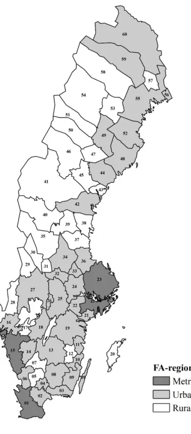
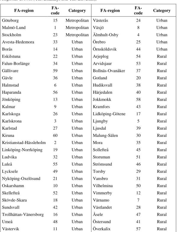
The purpose of this thesis is to examine the potential difference in job-matching efficiency between urban and rural functional analysis (FA) regions. A FA-region (hereafter denoted region) is usually constructed out of several municipalities and is designed to account for the fact that labor is spatially mobile and individuals who are living in one municipality do not necessarily have to work there as well since it is possible to commute to nearby mu-nicipalities.7 This thesis utilizes the latest (2015) categorization of Sweden’s 60 regions defined by Growth Analysis (Tillväxtanalys). Hence, this work follows Eklund et al. (2015) in the choice of base of the analysis.
The analysis of the job-matching efficiency will be done in two steps. The first step is to examine which factors that actually shift the curve in urban and rural regions. Similar to Bouvet (2012), the Beveridge curve will be estimated together with variables that are said to be included in the matching efficiency parameter A. As was discussed in the previous section there are several factors which shift the job-matching efficiency where education, age, sex, density and business cycles will be the focus of in this thesis. Hence, this equation will be estimated
𝑢𝑖𝑡 = 𝛽1+ 𝛽2𝑣𝑖𝑡+ 𝛽3𝑣𝑖𝑡2 + 𝛽4𝐸𝐷𝑈𝑖𝑡+ 𝛽5𝐴𝐺𝐸𝑖𝑡+
𝛽6𝑆𝐸𝑋𝑖𝑡+ 𝛽7𝐷𝐸𝑁𝑆𝑖𝑡+ 𝛽8𝐺𝐴𝑃𝑖𝑡+ 𝜀𝑖𝑡 (6)
where uit is the unemployment rate in region i at time t, vit is the vacancy rate, 𝑣𝑖𝑡2 is the
squared term of the vacancy rate to account for the curvature, EDU is the level of educa-tion, AGE is the average age, SEX is the share of women in the labor force, DENS is the population density and GAP is the output gap which is a proxy for business cycles. 𝜀𝑖𝑡 is the error term. Equation 6 will be estimated for Sweden as a whole and separately for urban and rural regions.
7 However, it is not uncommon that a region consists of only one municipality, e.g., the Haparanda region
includes only Haparanda municipality. Hence, such municipalities do not experience any significant amount of inter-municipality commuting.
13
The next step is to examine if shifts in the matching efficiency occur in the same years for both urban and rural regions. This is done by scrutinizing the year dummies which are included in the estimations of equation 6. As Wall and Zoega (2002) argue, the main in-terest of this method lies in the yearly differences of the dummy coefficients, since this allow one to observe if the Beveridge curve have shifted inward, outward or been immo-bile.
3.2 Data
This thesis employs a longitudinal dataset that consists of yearly data for the period 1998-2015 and which is obtained from either Statistics Sweden or the Swedish Agency for Eco-nomic and Regional Growth. To capture the regional job-matching efficiency, each region is classified as either an urban or rural region based on the three-type definition made by Growth Analysis (Tillväxtanalys, 2011).8 According to the definition, a region can either be metropolitan (storstadsregion), urban (täta regioner) or rural (landsbygdsregion) of which there are three, 32 and 25 regions, respectively. The starting point is to clarify what an urban area is, which is an area that have a population density of at least 300 inhabitants per square kilometer. In addition, a single square or a group of neighboring squares should have at least 5 000 inhabitants. Hence, rural areas are those kilometer squares which are not defined as urban areas. From this definition can the regional classifications be defined. A region is considered rural if the share of the population who lives within rural kilometer squares is at least 50 percent. A metropolitan region is defined as having a population share living in rural areas below 20 percent. Lastly, urban regions have between 20 and 50 per-cent of its population living in rural areas. Furthermore, if a region has a city with at least 200 000 inhabitants, the region is automatically considered an urban region. Likewise, if a region has a city with at least 500 000 inhabitants, the region is defined as metropolitan. Metropolitan and urban regions will in this thesis be considered urban while rural regions are rural. A map and a table over the different regions are provided in appendix 1.
8 These definitions are also available for municipalities (Tillväxtanalys, 2014). However, this thesis uses the
14
3.2.1 Variables
Unemployment rate
The dependent variable Unemployment rate is calculated as the regional number of openly unemployed aged 20-64 divided by the regional labor force. The data on open unemploy-ment is provided on regional level on quarterly intervals. To convert the data to yearly observations, the average number of unemployed per year is calculated.
Vacancy rate
The variable Vacancy rate denotes the regional stock of vacancies, i.e., both new and re-maining vacancies from t-1, relative to the labor force. As with unemployment, quarterly data on vacancies is obtain on regional level and the average number of vacancies per year is calculated. Since the Beveridge curve indicates a negative relationship between unem-ployment and vacancies, Vacancy rate is expected to be negative.
Vacancy rate2
Vacancy rate2 is the squared term of Vacancy rate. The variable is included in the
estima-tions to account for the convexity of the Beveridge curve. Given that the assumpestima-tions of convexity hold, Vacancy rate2 is positive.
Education
A region’s level of Education is measured as the number of individuals aged 20-64 who have finished at least tertiary education relative to the population. Based on the results from previous research (Badinger & Url, 1991; Bonthuis et al., 2013; Cole & Smith, 1996; Dur, 1996; Eklund et al., 2015), the expected relation between unemployment rate and education is ambiguous.
Age
Age measure the mean age of a region’s population. Data on the mean age is sourced on
municipality level, which are then weighted with the population size in each municipality and aggregated to regional level. As with Education, Age’s expected relation to the de-pendent variable is inconclusive.
15
Sex
The share of women in the labor force is measured by the variable Sex. A higher share is thought to indicate a less efficient job-matching and Sex is expected to be positive.
Output gap
Following both Kosfeld et al. (2008) and Bouvet (2012), the output gap is included in the estimations to account for business cycle fluctuations. The variable measures the percent-age difference between the real gross regional product, GRP, and the potential GRP. The potential GRP can be understood as the regional output level which is at its optimal full-capacity (Jahan & Mahmud, 2003) and sustainable in the long-term (i.e., where the infla-tion is constant; OECD, 2014). Although it is possible for regions to produce more than its full-capacity level, it is not sustainable as higher production comes with the cost of higher inflation.
While data on real GRP is available, the potential GRP must be calculated. This thesis utilizes the same method employed by both Kosfeld et al. (2008) and Bouvet (2012) in their calculations of the potential GRP and the output gap. Potential GRP is obtained by applying an Hodrick-Prescott filter to real GRP, where the filter basically decomposes the variable into a short-term cyclical and a long-term trend component. The trend can be con-sidered the potential GRP, which is the long-term trend that the regions have been on dur-ing the examined time period, 1998-2015. As mentioned in the literature review, Kosfeld et al. (2008) and Bouvet (2012) gives contradicting results and the expected effect of the output gap is thus unsure.
Density
The variable Density is employed to account for how populated a region is and measures the number of persons per square kilometer. The density is calculated by dividing the pop-ulation by land area. While Cole and Smith (1996) find that density is positive for the job-matching, Aranki and Löf (2008) point to the opposite for Sweden. Hence, the expected sign is ambiguous.
16
Table 1 – Description of variables
Variables
Description
Expected sign
Unemployment rate The number of openly unemployed aged 20-64 relative to the
la-bor force in region i
Dep. Var.
Vacancy rate The stock of vacancies relative to the labor force in region i -
Vacancy rate2 The squared term of vacancy rate in region i +
Education The proportion of the population in region i which has at least a
tertiarily education
+/-
Age The population average age in region i +/-
Sex The share of women in the labor force in region i +
Density The population in region i over the land area of region i +/-
Output gap The difference between real GRP and potential GRP relative to
potential GRP in region i
+/-
3.2.2 Descriptive statistics
The descriptive statistics for the whole dataset are presented in Table 2.9 The mean unem-ployment rate during the examined period was 5.7 percent. Nevertheless, large fluctuations can be observed where the lowest unemployment rate was 2 percent and the highest rate was 19.6 percent. The average vacancy rate during the period was 4.2 percent and there is again large variation. Education range from 2.9 to 20.5 percent with a mean of 8.3 percent. The variation in the regions’ population average age is relative to the other variables rather small, with an average of 43 years. The average share of women in the labor force is 47.3 percent with very small variation between the regions. Density is a variable which exhibits relatively large variations with a mean of 24.5 and median of 16.1 persons per square kil-ometer. This variation is also reflected by the large spread between the minimum and max-imum values, which range from 0.3 to 159 persons per square kilometer. Lastly, there is large deviation in the output gap, which vary from -39.0 percent to 26.1 percent. The av-erage output gap is slightly negative at -0.1 percent.
17
Table 2– Descriptive statistics FA-regions 1998–2015
Variables Mean Median SD Min Max
Unemployment rate 0.057 0.054 0.021 0.020 0.196 Vacancy rate 0.042 0.037 0.020 0.013 0.168 Vacancy rate2 0.002 0.001 0.003 0.000 0.028 Education 0.083 0.077 0.031 0.029 0.205 Age 43.070 42.851 2.000 37.616 49.400 Sex 0.473 0.473 0.010 0.448 0.502 Density 24.541 16.071 30.599 0.271 159.352 Output gap -0.001 -0.001 0.044 -0.390 0.261 3.2.3 Correlation analysis
A correlation matrix is found in Table 3. As predicted by the Beveridge curve, one can see that unemployment rate and vacancy rate are significantly and negatively correlated with each other. The same is true for the relation between the dependent variable and education,
density and output gap, respectively. Furthermore, unemployment rate is positive related
to age and sex. The correlation between density and education, and density and age are rather high, which might indicate the presence of multicollinearity. As a robustness check, a regression with density dropped will be estimated to see how the results changes.
Table 3 – Correlation matrix Unemploy -ment Vacancy rate Vacancy rate2
Educat-ion Age Sex Density
Output gap Unemploy. rate 1 Vacancy rate -0.223** 1 Vacancy rate2 -0.183** 0.947** 1 Education -0.403** 0.078* 0.005 1 Age 0.037 0.267** 0.237** -0.419** 1 Sex 0.119** 0.142** 0.074* 0.446** -0.224** 1 Density -0.151** -0.069* -0.092** 0.572** -0.587** 0.310** 1 Output gap -0.144** 0.104** 0.073* 0.034 0.017 -0.016 0.012 1
Source: own calculation based on data from Statistics Sweden and the Swedish Agency for Economic and Regional Growth
N=1080, n=60
**. Correlation is significant at the 0.01 level (2-tailed). *. Correlation is significant at the 0.05 level (2-tailed).
18
3.3 Econometric model
Given the longitudinal nature of the dataset, pooled ordinary least square (OLS) and fixed effect (FE) models are estimated. According to Gujarati and Porter (2009), in a pooled OLS all observations are pooled together, and the uniqueness of the observations are dis-regarded. As such, given its simplicity, the pooled regression does not account for the het-erogeneity among the different regions and assumes that the estimated coefficients are the same across the regions. Gujarati and Porter (2009) argue that such assumptions may not necessary hold. Therefore, the pooled OLS will in this thesis be considered as a benchmark for the other panel estimation model which will be employed. In contrast to the pooled OLS, the FE model controls for the unobserved time-invariant heterogeneity across the regions by letting each region have its own intercept (Gujarati & Porter, 2009). By em-ploying a FE model, the assumption that regions are homogenous can be neglected. It makes intuitionally sense that regions should differ from each other; for example, a region in the southern part of the country might be very different from a region in northern Sweden in ways which cannot be accounted for. Furthermore, a Hausman test is conducted which supports the use of a FE model.10
10 𝜒
19
4. Results
This section presents the results from the estimations based on the models outlined before. The results of the regressions including some of the determinants of unemployment will be discussed first. This is then followed by how the Beveridge curve have shifted in a Swedish, urban and rural perspective. Lastly, the robustness of the results will be tested.
4.1 Determinants of job-matching efficiency
This thesis is interested in examining if there is any difference between the job-matching efficiency in urban regions vis-à-vis rural ones. One method for observing such difference is to examine which factors are related to the unemployment rate in both types of regions, which this section will focus on. Table 4 present the results from the different iterations of equation 6, where the top-half shows the pooled regressions and the bottom-half shows the regressions with fixed effects. As was discussed before, the pooled regressions serve as a benchmark for which the estimations including fixed effect will be compared to. Hence, the results from the pooled regressions will be discussed just briefly. The regressions are estimated for the whole sample (denoted Sweden) and the urban and rural sub-samples, respectively. Furthermore, the regressions are also run with a specification for a “plain” Beveridge curve (i.e., with unemployment rate just dependent on vacancy rate and vacancy ratesquared) and with a specification including the variables which was introduced in the theory section. As such, 12 specifications in total will be estimated. It is also worthwhile to remember that, although the Beveridge curve is used to examine job-matching effi-ciency, equation 6 does not have job-matching as a dependent variable. Hence, the results in Table 4 are not explicitly related with matching efficiency. Nevertheless, the implication of the results on job-matching efficiency will be discussed in section 5.
Starting with the top-half of Table 4, one can see as predicted that the vacancy rate is negative for all regressions. Similar, vacancy ratesquared is as expected positive,
indicat-ing a curve which is convex towards the origin. The value for vacancy rate ranges from -.312 for Sweden with control variables (specification 2) to -.685 for urban regions without control variables (3). The relationship of vacancy rate weakens in all specification when the control variables are included in the estimations. In addition, the estimated coef-ficients for vacancy rate are all significant on at least 0.05 percent level, with the exception of specification 4.
20
Table 4 – Dependent variable: Unemployment rate
(1) Sweden (2) Sweden (3) Urban (4) Urban (5) Rural (6) Rural VARIABLES Vacancy rate -0.514*** -0.312*** -0.685*** -0.272 -0.343** -0.626*** (0.098) (0.089) (0.258) (0.219) (0.138) (0.109) Vacancy rate2 2.128*** 0.682 2.801 2.141 0.958 2.186*** (0.717) (0.628) (2.731) (2.242) (0.910) (0.703) Education -0.414*** -0.459*** -0.527*** (0.023) (0.028) (0.043) Age -0.001 -0.004*** 0.000 (0.000) (0.001) (0.001) Sex 0.902*** 1.015*** 0.754*** (0.061) (0.082) (0.086) Density 0.000 -0.000* -0.001*** (0.000) (0.000) (0.000) Output gap -0.044*** -0.044*** -0.052*** (0.012) (0.016) (0.016) Constant 0.074*** -0.301*** 0.077*** -0.220*** 0.073*** -0.249*** (0.003) (0.033) (0.006) (0.046) (0.004) (0.051) Observations 1,080 1,080 630 630 450 450 R-squared 0.057 0.351 0.083 0.410 0.059 0.483
Region & year FE NO NO NO NO NO NO
VARIABLES (7) Sweden (8) Sweden (9) Urban (10) Urban (11) Rural (12) Rural Vacancy rate 0.025 -0.240*** -0.118 -0.320** 0.072 0.024 (0.079) (0.071) (0.198) (0.150) (0.010) (0.099) Vacancy rate2 -0.386 0.674 -0.968 0.288 -0.252 -0.345 (0.578) (0.517) (1.824) (1.378) (0.657) (0.651) Education 0.232*** 0.410*** 0.188 (0.073) (0.088) (0.171) Age -0.011*** -0.016*** -0.006*** (0.001) (0.001) (0.002) Sex 0.509*** 0.938*** 0.384*** (0.064) (0.110) (0.086) Density -0.000 -0.001*** -0.001 (0.000) (0.000) (0.003) Output gap -0.004 0.003 -0.012 (0.007) (0.008) (0.012) Constant 0.084*** 0.306*** 0.086*** 0.318*** 0.085*** -0.169** (0.002) (0.056) (0.005) (0.095) (0.004) (0.067) Observations 1,080 1,080 630 630 450 450 R-squared 0.644 0.732 0.621 0.795 0.692 0.718
Region & year FE YES YES YES YES YES YES
Standard errors in parentheses *** p<0.01, ** p<0.05, * p<0.1
21
The control variables are in general statistically significant except for age. However, while density is significant two of the specifications, the estimated coefficients are very small and the relationship with unemployment rate might not be significant in an eco-nomic sense.
By including regional and year fixed effects in the regressions (which are shown in the lower part of Table 4), one can observe that the R-squared’s are higher which can be seen as the descriptive power of the models increase. Unlike the pooled regressions, vacancy
rate is not significant in all specifications. Vacancy rate squared is never significant and
exhibits the expected sign in only two specifications (8 and 10).
The continued presentation of Table 4 shows that education is positively related to un-employment rate in Sweden and urban regions, and hence increases unun-employment. The mean age in a region is negatively associated with the dependent variable for the both urban and rural regions, and Sweden as a whole. The share of women in the labor force,
sex, is expected to be positive and the results in Table 4 support this theory. Sex is positive
in all regions and highly significant in all specifications. Lastly, both density and output
gap are clearly insignificant with the exception of urban regions, where density is
signif-icant.
As seen in Table 4, there appears to be some difference between urban and rural regions in terms of job-matching efficiency. Table A.4 in the appendix includes interaction terms between the control variables and an urban dummy, which allows one to see if there is a significant difference between the estimated relationship in urban and rural regions. Table A.4 confirms the observed difference between the two types of regions in Table 4 regard-ing education. Furthermore, both age and sex are more related to the unemployment rate in urban regions compared to rural ones. However, there is no significant difference in the unemployment rate, which is indicated by the urban dummy in Table A.4.
22
4.2 Movement of the curve
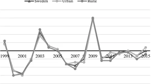
While previous section has examined the relationship between the selected determinants and the unemployment rate, this section focuses instead on how the Beveridge curve has shifted during the examined time period in urban and rural regions. Table 5 present the results from the estimation of equation 6 with the coefficients for the year dummies re-ported for Sweden as whole and urban and rural regions, respectively. By following Wall and Zoega (2002) and calculating the yearly changes of the dummy coefficients, one is able to see if the Beveridge curve has shifted. If the change between two dummy coeffi-cients is positive, the curve is then considered to shift outwards for that year. Likewise, a negative value is associated with an inward movement.11
Figure 2 shows the calculated changes in the coefficients. Values above the 0-mark indi-cate an outward shift while values below indiindi-cate an inward shift. Several interesting ob-servations can be made from Figure 2. First of all, the changes in the regional labor mar-kets efficiency correlate strongly between the urban and rural regions. The movement of the curve for the two types of regions also corresponds to that of the aggregated national labor market. Furthermore, the Beveridge curve has shifted direction several times during the examined time period. The curves shifted inwards during the years 2000-2002. For the period 2003-2005 the curve shifted outwards but improved from 2006 until the finan-cial crisis. It is interesting, but expected, to see that curve moved greatly outwards during the crisis. However, the crisis seems not to have any prolonged effects on the labor mar-ket, as the curve started to move inwards again 2010. The subsequent period exhibits relative stable curves for the different regions. Table 6 summarize the movement of the Beveridge curve. One can see that both type of regions and Sweden have shifted simul-taneous during this time with only a few exceptions.
11 For example, consider the difference in the dummy coefficients for Sweden between 2002 and 2003. The
change in the coefficient between those years is -0.015 - (-0.026) = 0.011. Since 0.011 is a positive value, the Beveridge curve shifted out between 2002 and 2003.
23
Table 5 – Dependent variable: Unemployment rate
(1) Sweden (2) Urban (3) Rural VARIABLES Vacancy rate -0.240*** -0.320** 0.024 (0.071) (0.150) (0.099) Vacancy rate2 0.674 0.288 -0.345 (0.517) (1.378) (0.651) 1999 0.005*** 0.004** 0.006** (0.002) (0.002) (0.003) 2000 -0.007*** -0.008*** -0.009*** (0.002) (0.002) (0.003) 2001 -0.021*** -0.023*** -0.023*** (0.002) (0.003) (0.003) 2002 -0.026*** -0.028*** -0.029*** (0.002) (0.003) (0.004) 2003 -0.015*** -0.019*** -0.016*** (0.003) (0.004) (0.004) 2004 -0.012*** -0.016*** -0.014*** (0.003) (0.004) (0.005) 2005 -0.011*** -0.015*** -0.014*** (0.003) (0.004) (0.005) 2006 -0.019*** -0.023*** -0.022*** (0.003) (0.005) (0.006) 2007 -0.028*** -0.030*** -0.033*** (0.004) (0.005) (0.006) 2008 -0.033*** -0.037*** -0.036*** (0.004) (0.006) (0.007) 2009 -0.013*** -0.018*** -0.016** (0.004) (0.006) (0.007) 2010 -0.017*** -0.023*** -0.022*** (0.004) (0.006) (0.007) 2011 -0.021*** -0.024*** -0.028*** (0.005) (0.007) (0.008) 2012 -0.022*** -0.026*** -0.029*** (0.005) (0.007) (0.008) 2013 -0.022*** -0.026*** -0.030*** (0.005) (0.007) (0.008) 2014 -0.025*** -0.029*** -0.035*** (0.005) (0.008) (0.009) 2015 -0.025*** -0.027*** -0.037*** (0.005) (0.008) (0.009) Constant 0.306*** 0.318*** 0.159* (0.056) (0.095) (0.083) Observations 1,080 630 450 R-squared 0.732 0.795 0.718
Region FE YES YES YES
Note: Control variables included but not reported. Standard errors in parentheses *** p<0.01, ** p<0.05, * p<0.1
24
Figure 2 – Change in the intercept of Beveridge curve
Table 6 – Movements of the Beveridge curve
Year Sweden Urban Rural
1999 → → → 2000 ← ← ← 2001 ← ← ← 2002 ← ← ← 2003 → → → 2004 → → - 2005 → → ← 2006 ← ← ← 2007 ← ← ← 2008 ← ← ← 2009 → → → 2010 ← ← ← 2011 ← ← ← 2012 ← ← ← 2013 - - ← 2014 ← ← ← 2015 - → ← -0.02 -0.015 -0.01 -0.005 0 0.005 0.01 0.015 0.02 0.025 1999 2001 2003 2005 2007 2009 2011 2013 2015 C ha ng e in i nter ce pt of B eve ridg e curve Year
25
4.3 Robustness checks
Table A.5, A.6 and A.7 in the appendix show three additional specifications based on equation 6 in order to examine the robustness of previous results. The first specification omit density since this variable is rather correlated with both education and age, as shown in Table 3. Failure to acknowledge that these variables are correlated could give biased results due to multicollinearity. However, when omitting density, there are no dramati-cally changes in the results. The main difference in the pooled estimations is that age now is significant for rural regions and nationally. When including regional fixed effects,
va-cancy rate is insignificant for urban regions.
The second specification include vacancy rate with a one-year lag, t-1. The rationale be-hind including vacancy ratet-1is that it might take some time between a vacancy is posted
and until it is filled, which lower the unemployment rate. Nevertheless, by using yearly data, there should be enough time for vacancies to get filled and there should not be any major effect by employing a lag on the vacancy rate. However, vacancy ratet-1 is
insig-nificant for urban regions without control variables. For the fixed effect models, there are some minor differences compared to when not using vacancy ratet-1.
Lastly, the third specification omits the three metropolitan regions in Sweden: Stockholm, Gothenburg and Malmö. The intuition is that the labor markets in these regions might be very different due to their size compared to the other regions. Since time-invariant re-gional characteristics are controlled for by the fixed effect model, it is not expected to be any differences in the results when these three regions are omitted in the that kind of regression. Furthermore, no major differences are found in the pooled regressions.
26
5. Discussions
The purpose of this section is to connect the results from this thesis with the findings from previous studies and discuss the results in a broader perspective.
The results in the previous section provide further insight on the job-matching efficiency in Swedish regional labor markets. As the main theory behind the Beveridge curve is that there is a negative relationship between unemployment and vacancy, it is interesting to find that this relationship to some extent also holds in a Swedish context. The results also support previous findings made by Eklund et al. (2015) regarding the relationship be-tween the unemployment rate and the vacancy rate in Sweden.
5.1 Discussion on the determinants of unemployment
Focusing on the results from the FE models, it is not surprising to find that education is a significant factor for unemployment. Hence, by employing the Beveridge curve as a the-oretical framework, education seems to be related to the job-matching efficiency, as ar-gued by Blanchard and Diamond (1989). However, there is no clear consensus in previous literature whether education increases or decreases the efficiency of the labor market. The results in this thesis suggest that education is positively related to unemployment and subsequently reduces the matching efficiency. Petrongolo and Pissarides (2001) state that mismatch is due to the skills offered by the labor force differ from the skills demanded by the firms. As such, it might be that the education held by the Swedish workers do not correspond to what the firms require, at least not in urban regions, and the job-matching efficiency decreases. This explanation contradicts the findings of Eklund et al. (2015), which have shown that the Swedish job-matching efficiency for low-skilled labor is rel-atively worse. However, the outcome of this thesis does not necessarily suggest that edu-cation per se is bad for the job-matching efficiency, as this thesis neglects any heteroge-neity among higher education. For example, consider a region where any person who has a higher education is an economist. This region would have a low job-matching efficiency if the hiring firms only demanded engineers.
Nevertheless, the decreased efficiency which is due to education could also imply that firms require low-skilled workers. Similarly, Cole and Smith (1996) have found that ed-ucation decreases the matching efficiency while a large share of firms within the
27
manufacturing industry improved the matching in their examination of the British labor market. They argued that the manufacturing industry demand low-skilled labor, which increases the mismatch from education. Hence, while it seems unlikely, it could be that the Swedish firms do not demand educated labor.
Another explanation for the positive relation between education and unemployment could be due to how the data on vacancies is collected. As data on vacancies only includes vacancies that firms actually announce to the Swedish public unemployment service, it neglects the vacancies which are not announced. Furthermore, the data employed does not include information on what kind of labor the firms are searching. Hence, a more far-fetched explanation for why education decreases the job-matching efficiency is that the vacancies which are announced to the public unemployment service are jobs which do not require a higher education. While this explanation is not testable given the current data, it lends nevertheless some support for why the results indicate that education shifts the Beveridge curve outwards.
The results in Table 4 show that both the other demographic characteristics included, the regions’ mean population age and the share of women in the labor force, are significant factors for the unemployment rate in both types of regions. The age composition is nega-tively associated with the dependent variable, indicating that an older population reduces unemployment and can be seen to shift the Beveridge curve inwards. This result is par-tially in favor of Bouvet (2012), who argues that young people reduce the job-matching efficiency. However, this thesis contradicts Boethius et al. (2013), which note that young-ster is less specialized and thus have less obstacles to find a job.
One potential reason why a younger population is related a higher rate of unemployment is that it is harder for youngster to find a job. Likewise, an older population might find it easier to obtain a job. Hence, there might be some underlying aspects which differentiate younger and older individuals’ job-matching efficiency. One such aspect could be that younger persons lack the required experience which the hiring firms demand. It is natural that individuals in their prime age have had more years to accumulate both experience and skills compared to youngsters. Hence, the recruiting firms might prefer to hire older persons which have more experience. Another factor can be discrimination of youngster in comparison with older individuals. While discrimination might steam from prejudices
28
against younger persons reduced capabilities due to a lack of experience, discrimination could also be because of a general unwillingness to hire youngsters.
Given that previous research has shown that women might find it harder to find a job (e.g., Börsch-Supan (1991), Samson (1994) and Bouvet (2012)), it is not surprising that
sex, the share of women in the labor force, is positively related to unemployment. Hence,
according to the Beveridge curve, sex decreases the job-matching efficiency. While Sam-son (1994) argues that women might be less attached to their jobs because they are less qualified or due to maternity, Bouvet (2012) fails to elaborate on this subject. If it is true that women have a less direct relationship with their workplaces, it is in that case im-portant to understand why. There are several potential reasons why women show less attachment. It could be true as Samson (1994) argues that women are less qualified then men. However, as education is positively related to unemployment, Samson’s (1994) ar-gument is not supported in this thesis. If women were less qualified, they would probably have a lower level of education. As such, a higher share of women in the labor force should reduce the unemployment rate.
A more plausible reason for women’s lower attachment to their jobs could be due to ma-ternity, which is also noted by Samson (1994). As such, women need to be absence from work during part of the pregnancy and the subsequent parental leave. In addition, women with child might choose to reduce the number of working hours during the childhood years. Given that women are less attached to their job’s due to maternity, it is not too far-fetched that a higher share of women in the labor force increases the unemployment. Another reason for women being positively related to unemployment could be due to traditional gender roles, where it is the men who are expected to proceed a career rather than women. Women might then have less incentives to be involved to a higher degree in the labor market. However, while this explanation would have been more plausible 50 years ago, it is unlikely that women today are not interested in their careers and such explanations are hence less valid in the examined spatio-temporal context.
A third explanation for the positive relation between women and unemployment is crimination of women on the labor market, which is related to the both previously dis-cussed reasons. While gender roles probably are less prominent in the labor market today, it is possible that latent gender roles still exist. Hence, employers might be more prone to
29
discriminate women. It is also possible that employers chose to not employ women as women are more likely to be away from work for longer period due to maternity. It is also interesting to observe that neither density nor output gap are significant factors in explaining unemployment. Previous articles (Aranki & Löf, 2008; Cole & Smith 1996) have found that density is significant in the matching process. However, such articles have employed a different model, where the number of matches is dependent on vacancy and unemployment. Hence, the discrepancy in the results is likely due to the choice of empirical framework. Lastly, other authors (Bouvet, 2012; Kosfeld et al., 2008) have ar-gued that cyclical fluctuations are an important factor for the movement of the Beveridge curve. This thesis does not find that business cycles, measured as the output gap, are significant. A possible reason is that, while cyclical fluctuations is related to unemploy-ment in the countries which previous research has examined, such fluctuations is simple not a significant factor in Sweden.
5.2 Discussion on the movement of the curve
Based on previous literature (e.g., Cole and Smith (1996) and Aranki and Löf (2008)), one might expect that the movements of the Beveridge curve, and hence job-matching efficiency, would differ for urban and rural regions. However, Wall and Zoega’s (2002) examination of the job-matching efficiency in ten British regions12 shows a rather uni-formed development for the different kinds of regions.13 While the authors do not dis-cusses their results in terms of “urban” and “rural”, it is likely that there are some regions which are more characterized as rural ones. At the same time, some regions are probably relative more urban. Furthermore, Wall and Zoega (2002) do not elaborate on their results on why they observe a similar pattern across the regions.
One can nevertheless speculate why the shifts of the aggregated, urban and rural Beve-ridge curve are correlated with each other. A possible reason is that each types of region are following a general development of the job-matching efficiency. For example, both
12 These regions are: North, Yorkshire and the Humber, East Midlands, East Anglia, South East, South
West, West Midlands, North West, Wales and Scotland.
13 It is important to emphasize that both Wall and Zoega’s (2002) and the analyze in this section are
con-sidering the change in job-matching efficiency, i.e., shifts in the Beveridge curve. On the other hand, Cole and Smith (1996), and Aranki and Löf (2008) are discussing the absolute matching efficiency.
30
urban and rural regions were affected by the financial crisis 2008, and the labor market for both types of regions recovered from the crisis in a similar pace. As such there was an incident, the crisis, which impacted the Swedish labor market, of which both urban and rural regions are part of. Although the financial crisis 2008 might be considered an ex-treme example, it is not unlikely that similar but less exex-treme events have affected the labor market throughout the years which give rise to a general development of the job-matching efficiency. While it can be difficult to explain the correlated movement of the Beveridge curve for urban and rural regions, it is simpler to explain why both kinds of regions shift synchronized with the national curve. Since the national Beveridge curve is aggregated on the regional labor markets, it is not surprisingly that movements of the national curve are correlated with the regional ones.
Since Eklund et al. (2015) employ a different method for observing shifts in the job-matching efficiency, it is not possible to compare the result in Figure 2 and Table 6 di-rectly with those of Eklund et al. (2015). Nonetheless, Eklund et al. (2015) plot the na-tional Beveridge curve and indicate the shifts which they observe. They found that the job-matching efficiency increased for the period 1995-2000, which roughly corresponds to the results shown in Figure 2 and Table 6. The subsequent period in Eklund et al. (2015), 2001-2014, exhibits three inwards and two outwards shifts and it is interesting to note that similar shifts are found is this paper as well.
5.3 Limitations
This thesis aims to examine if there is a difference in the job-matching efficiency between urban and rural regions in Sweden. The results in previous section suggest that there are indeed some differences between the two types of regions. There is however no signifi-cant difference in the position of the Beveridge curve, as indicated by the urban dummy in Table A.4. According to the Beveridge curve, this implies that the job-matching effi-ciency is similar in both urban and rural regions. Furthermore, the movement of the curve appears to correlate between regions. Based on previous research (Aranki & Löf, 2008; Cole & Smith, 1996; Duranton & Puga, 2003), one would expect it to be a more pro-nounce disparity between urban and rural regions. One reason why this thesis does not find the expected difference in the job-matching efficiency could be due to how the re-gions are defined. With the definitions made by Growth Analysis (Tillväxtanalys, 2011),
31
several regions which are not typically recognized as urban are categorized as such. To mitigate the potential problem with the current regional definition, one could employ a different set of definitions. While there are no other urban/rural definitions based on FA-regions, Growth Analysis have defined the Swedish municipalities from an urban/rural perspective. Nevertheless, these definitions are similar to the ones used for FA-regions (cf. Tillväxtanalys, 2011, 2014). For example, Haparanda is in general opinion usually thought of as being a rural region and municipality, but Growth Analysis defines Hapa-randa as urban. While there exist other urban/rural definitions for municipalities (e.g., the Board of Agriculture (Jordbruksverket, 2013)), using municipalities as a base for analysis poses other difficulties. It is likely that several variables exhibit spatial autocorrelation across municipality boundaries, which produces inefficient estimates and makes it more likely to find insignificant results.
Further limitation includes the theory of the Beveridge curve itself. As previous literature has argued, the intuition behind the theory is that an increase (decrease) in the unemploy-ment for a given level of vacancies shift the curve outwards (inwards) and the job-match-ing becomes less (more) efficient. While several other articles have employed the curve as a theoretical framework for examining job-matching efficiency, matching efficiency do not explicitly enter the estimated function. Some articles (e.g., Coles and Smith (1996), Dur (1999), Aranki and Löf (2008), and Eklund et al. (2015)) have in their studies on job-matching efficiency employed a model where the number of matches is a function of unemployment and labor (similar to equation 2). In such equations the matching effi-ciency enters the model explicitly and it might make more sense (compared to the Beve-ridge curve) to talk in terms of factors which are directly related to job-matching effi-ciency. However, the number of matches has not been available for this thesis which prevent the employment of such models. Nevertheless, according to the literature pre-sented in section 2, the Beveridge curve is a commonly applied theory when examining the efficiency of the job-matching process.
While data availability in general is good in Sweden in an international comparison, the lack of certain data prohibits a more thoroughly analysis of the job-matching efficiency. Another theoretical framework might have been more appropriate if, as mentioned, infor-mation on matches was accessible. Furthermore, it is useful to keep in mind that the anal-ysis is performed on an aggregated level. As such it might be difficult to interpret how
32
individual characteristics correlate with matching efficiency. It would also been desirable to have data on microlevel, where one could see the characteristics of each individual and firm. If microdata on actual matches between unemployed and vacancies were available, it would also be possible to examine the quality of the matches that occurs; it is thinkable that an individual can be employed even though it is not a perfect match. Lastly, as was noted in the discussion on education, it would be beneficial for future research to include a more diverse measure of education which takes into account different types of educa-tion, such as economics and engineering.