Determinants of forex market movements during the European sovereign debt crisis: The role of credit rating agencies.

Determinants of forex market movements during the

Europe-an sovereign debt crisis:

The role of credit rating agencies.

Master’s Thesis within Economics and Finance

Author: Marharyta Karpava

Professor: Andreas Stephan

Master’s Thesis in Economics and Finance

Title: Determinants of forex market movements during the European Sover-eign debt crisis: The role of credit rating agencies.

Author: Marharyta Karpava

Tutor: Andreas Stephan

Date: 2012-06-11

Subject terms: Credit rating, sovereign debt crisis, Euro depreciation, event study.

Abstract

The purpose of this thesis is to identify key factors underlying exchange rate develop-ments during the European sovereign debt crisis by examining the impact of credit rat-ing news, published by the three leadrat-ing credit ratrat-ing agencies, on conditional returns and volatility of EUR/USD (direct quotation) exchange rate. Empirical results highlight the importance of interest rate differential and volatility index of options exchange in explaining EUR/USD exchange rate volatilities. Downgrade announcements by Stand-ard & Poor’s as well as watch revisions by Fitch Ratings had a detrimental impact on the value of Euro, leading to a subsequent Euro depreciation over the period under con-sideration (January 2009 – April 2012).

Table of Contents

1

Introduction ... 1

2

Background information and literature review ... 4

2.1 Credit ratings industry ... 4

2.2 Role of credit rating agencies in financial markets ... 5

2.3 Accuracy of sovereign default assessment ... 6

2.4 Sovereign credit ratings and financial crisis ... 7

3

Methodology ... 9

3.1 Exchange rate determination ... 9

3.2 Event study methodology ... 11

3.3 Motivation for the application of EGARCH model ... 12

3.4 Regression model specification ... 14

3.5 Empirical framework ... 15

4

Data and preliminary analysis ... 16

5

Empirical results ... 18

5.1 Benchmark regression ... 18

5.2 Reactions to Standard & Poor’s credit rating announcements ... 19

5.3 Reactions to Fitch Rating’s credit rating announcements ... 22

5.4 Reactions to Moody’s credit rating announcements ... 24

5.5 Limitations and implications for further research ... 27

6

Conclusion ... 28

References ... 30

1

Introduction

By reading daily news since summer 2007, one might get an impression that many developed economies across the world are suffering from one long-lasting financial crisis; however, in reality that is not the case. The global financial turmoil started in the United States with the real estate bubble in the summer of 2007, which affected numerous financial institutions that invested substantial funds in mortgage-backed securities, thereby leaving banks with liquidity and solvency problems, and eventually resulting in a banking crisis. As a result, stock markets crashed in September 2008 (following the collapse of Lehman Brothers), leading to a subsequent contraction of wealth, GDP and fiscal income, thus, forcing governments to intervene and initiate safety plans to rescue financial institutions. For example, in the period from October 2008 through May 2010, approximately 200 banks from 17 countries contributed around 1 trillion Euros to government guarantee programs (Levy & Schich, 2010). The Eurozone, in its turn, contributed around 23% of its GDP to financial sector bailouts (Attinasi, Checherita, & Nickel, 2009). Government stabilization programs and domestic demand shrinkage caused governments to take on more debt, which increased country risk and probability of default, leading to a sovereign debt crisis in the Eurozone. For instance, Irish government bond spreads rose significantly after the announcement of a government guarantee for bank bonds (Sgherri & Zoli, 2009).

The sequence of crisis linkages did not stop here, but rather transformed into a currency crisis as spreads on government bonds of affected countries rose, thereby weakening balance sheets of the central banks. As a matter of fact, these tensions led to domestic currency depreciation in the troubled countries, US dollar and Euro, for example. In the view of high uncertainty about future dynamics of the domestic currency, any unfavorable macroeconomic announcements could lead to further currency depreciation. Therefore, financial market speculators could take advantage of the unstable position of the Euro currency and exploit possible arbitrage opportunities, leading to a self-fulfilling currency crisis (Candelon & Palm, 2010). Credit rating agencies, in their turn, might also contribute indirectly to further Euro depreciation by publishing negative watch lists and outlooks for countries within the European Monetary Union. Therefore, the role of the credit rating agencies in this vicious cycle will be closely examined in this paper.

Sovereign credit ratings have a large economic impact as they tend to increase the magnitude of business cycles, because ratings are upgraded during expansionary periods and downgraded during contractionary periods. Thus, any negative credit rating signals have a detrimental effect on a sovereign’s economy by limiting the number of credit sources available, thereby making debt and interest payments more costly. Portfolio managers are forced to get rid of the downgraded securities due to the legislative requirements (many government-owned financial institutions are prohibited from investing funds into below investment-grade assets), thereby worsening already existing imbalances in financial markets. In addition to this, sovereign credit ratings often set a limit to corporate ratings assigned to financial institutions, which are operating in that country. Thus, negative credit rating announcements do not only weaken the financial position of a sovereign on the macroeconomic level; the impact of negative sovereign news is also well observed on the microeconomic level.

Problem discussion

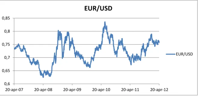
By looking at the graph of daily spot exchange rate movements over 60 consecutive months, it is fairly obvious that Euro was relatively stable until the middle of 2008, when the global economy was hit by the US stock market crash following the collapse of Lehman Brothers in September 2008. The volatility did calm down for a while until the beginning of 2009, owing mostly to central banks’ rescue packages for financial sectors to prevent collapse of the affected institutions, thereby contributing to stabilization of the global economic activity and subsequent Euro appreciation. Euro began depreciating at the end of 2008 - beginning of 2009, when credit rating agencies started downgrading Greek and Irish sovereign bonds in the view of high budget deficits. The Euro began falling again in the last quarter of 2009 up until the beginning of June 2010. This period of extensive Euro depreciation was largely affected by rising public debt levels in Greece, Ireland, Portugal and Spain, which were reflected in negative sovereign rating events, published by each credit rating agency within this time frame. There was a sudden slump in the value of the domestic currency (Euro) around the end of 2010 until the beginning of 2011, when S&P and Fitch assigned junk bond rating to Greek government bonds. The Euro began depreciating again in the second quarter of 2011 up until the beginning of January 2012, when a series of negative watch and outlook revisions were announced by S&P and Fitch, followed by massive downgrade announcements for Eurozone countries in the early January 2012.

According to the statistics data obtained from the Federal Reserve Bank of New York1, the Euro suffered from 20% drop in value over a 7 month-period in 2009-2010 (Euro-currency decreased from 1.4999 USD on 9 November 2009 to 1.19976 USD on 4 June 2010, thereby reaching its five-year absolute minimum). In addition to this, the Euro suffered from 13% decline in value over the 8 month-period in 2011-2012 (Euro-currency declined from 1.462499 USD on 26 April 2011 to 1.2723 USD on 5 January 2012)..

Figure 1-1: Spot exchange rate movements, 20 April 2007 – 20 April 2012.

1 _{Federal Reserve Bank of New York official website: http://www.federalreserve.gov/default.htm.}

0,6 0,65 0,7 0,75 0,8 0,85

20-apr-07 20-apr-08 20-apr-09 20-apr-10 20-apr-11 20-apr-12

EUR/USD

Purpose

The purpose of this paper is to identify main factors, underlying euro-dollar exchange rate fluctuations during the European sovereign debt crisis. One of the primary objectives is to de-termine the impact of sovereign credit rating announcements, if any, published by the three leading credit rating agencies (Standard & Poor’s, Moody’s and Fitch Ratings), on the condi-tional mean and volatility of the spot exchange rate USD/EUR (indirect quotation). The im-pact of credit rating announcements will be examined on an individual basis, thereby allowing to determine the impact of each credit rating agency on the volatility of Euro during the sov-ereign debt crisis.

To date, this is one of the first papers to study the impact of sovereign credit rating an-nouncements on foreign exchange markets. This paper employs an event-study methodology, which was used by many academic scholars in the past to examine the following: the impact of credit rating news on bond and equity markets, as well as, the effect of macroeconomic public announcements on foreign exchange markets.

Contributions

While the impact of credit rating announcements on stock and bond markets received a great deal of attention among academic scholars in the past2, existing literature that examines the relationship between sovereign credit ratings and foreign exchange markets remains scarce. This work, thus, complements existing research on the role of credit rating agencies in international financial markets and makes a valuable contribution to understanding the impact of credit rating news on the volatility of foreign exchange rates. This paper extends existing literature by examining the relationship of sovereign credit rating events and high frequency forex markets by focusing on response reaction of the spot exchange rate USD/EUR during periods of financial distress, thereby allowing to determine the crucial role of credit rating agencies in international finance.

The remainder of this paper is organized as follows. Section 2 provides background information and discusses prior research findings. Section 3 describes methodology and provides an overview of the theoretical framework and empirical strategy. Section 4 describes data. Section 5 discusses empirical findings, interprets the results, elaborates on the limitations of the study and provides recommendations for further research. Section 6 concludes.

2 _{See (Cantor & Packer, 1996), (Brooks, et al., 2004), (Reisen & von Maltzan, 1999), (Elayan,}

2

Background information and literature review

This section provides a thorough description of credit ratings industry discusses the impact of credit rating announcements on financial markets and sheds a light on previous research find-ings relevant to the objectives of this paper.

2.1

Credit rating industry

Credit ratings industry is dominated by the three leading credit rating agencies, which include Standard and Poor’s (S&P) [you may want to change this to (S&P) for clarification of posses-sive pronoun], Moody’s Investor Service and Fitch Ratings. Rating agencies assign a grade to the bond issuer according to the relative probability of default, which is measured by the country's political and economic fundamentals. Credit rating agencies distinguish between an investment grade rating, which varies from “AAA” (Fitch’s and S&P's) or “Aaa” (Moody's) to “BBB-“(Baa3), and a speculative grade rating, or “junk” bond rating, which consists of high yield bonds, where higher interest rates on debt serve as a compensation for greater amount of risk associated with lending to the sovereign with questionable creditworthiness. Speculative grade conveys the scale range from “BB+” (Ba1) and below up until “D” (Fitch and S&P's) or “C” (Moody's). Even though the three credit rating agencies use different rating scales of measurement, there is a high degree of correspondence between them. A table with a corresponding explanation of rating grades, assigned by each CRA, is listed in the Appendix. Credit ratings tend to differ among CRAs, which can be mainly attributed to different estima-tion methodologies and proxy variables, considered in the analysis. Background informaestima-tion and discussion of major differences in default probability assessment will follow below. Standard and Poor’s Ratings is the world’s largest credit rating agency, which dates back to as early as 1860 when Henry V. Poor’s “History of railroads and canals of the United States” book was released. Mr Poor is one of the early proponents of making financial information publicly available to potential investors. In 1941 Poor’s publishing company merged with Standard Statistics, forming Standard & Poor’s. Today S&P is a subsidiary of McGraw-Hill Financial, which comprises of S&P Equity Research, S&P Valuation and Risk Strategies, and S&P Indices. The company is headquartered in New York and reported a combined revenues of 2.9 billion USD in 2010 in accordance with the S&P’s statistics data obtained from the of-ficial website.

Moody’s Investor Service is another US-based credit rating agency, headquartered in New York. It was founded in 1909 by John Moody with an objective to publish statistics manuals of stock and bond ratings. Today it is a subsidiary of Moody’s Corporation, which also in-cludes Moody’s Analytics. Combined revenues equalled to 2.03 billion USD in 2010 accord-ing to the statistics data provided on the company’s website.

Fitch Ratings is the smallest of the big three credit rating agencies, which traces its history back to 1913 when John K. Fitch founded the Fitch Publishing Company in New York City. The company’s main objective was to provide financial statistics on stock and bond ratings. In 1924 the company first introduced the ordinal scale of “AAA” through “D” format, used up until this day. Fitch Ratings was the first among the big three to get recognition from the Se-curities and Exchange Commission as a nationally recognized rating organization (NRSRO) in as early as 1975. Today Fitch Ratings is a part of the Fitch Group, which is dual-headquartered in London, UK and New York, USA and jointly owned by FIMALAC and

Hearst Corporation. According to the statistics data3, provided on the official website, Fitch Ratings reported revenues of 487.3 million Euros (656.9 million USD) in 2010.

Getting back to the differences in credit default assessment among the big three CRAs, S&P focuses mostly on the forward-looking probability of default. Moody's bases its rating deci-sions on the expected loss, which is a function of both the probability of default and the ex-pected recovery rate. Finally, Fitch takes into consideration the probability of default and the recovery rate, as well.

One more reason that explains differences in credit ratings across the CRAs is the lack of pub-licly available information as to how CRAs assign weights to each variable they consider in assessment of the credit risk. Generally, the following factors are taken into consideration by the three CRAs when making credit risk assessment: economic and political factors, fiscal and monetary indicators and debt burden.

2.2

Role of credit rating agencies in financial markets

Sovereign credit ratings are perceived by the market participants as important indicators of a country risk, future economic development and financial stability. Hence, a rating downgrade will generally affect the country's financial austerity policies by raising corporate taxes to be able to afford borrowing at a higher cost, thereby reducing corporate cash flows and pushing down stock prices that might shatter investor confidence and eventually lead to a massive sell-off of the domestic currency, contributing to local currency depreciation. Therefore, the market impact of negative credit rating events might have a detrimental effect on the economic development of a sovereign and its financial market structure.

Previous studies on sovereign credit ratings find that rating events convey important information to financial markets4. The asymmetric effects of credit ratings have been studied explicitly by many researches ( (Brooks, Faff, Hillier, & Hillier, 2004), (Kim & Wu, 2011), (Kräussl, 2005)), reporting that only rating downgrades and negative outlooks have economically and statistically significant effects on debt and equity markets in contrast to rating upgrades and positive outlooks, which have weak or insignificant impact on financial markets. Several research papers also find evidence of strong contagion effects5 of watch and outlook changes on stock, bond and CDS markets of nearby countries ( (Gande & Parsley, 2005), (Ferreira & Gama, 2007), (Ismailescu & Kazemi, 2010)). Cantor and Hamilton (2004) and Alsati et al. (2005) find evidence that rating events are good predictors of future dynamics of sovereign credit rating announcements, as they shed a light on which government bond issuers are likely to default on their debt or to be downgraded in the foreseen future.

Spillover effects refer to short-term contagion across countries and financial markets. This

topic has been studied extensively by many researchers. Most studies report significant spillover effects across sovereign ratings (see (Gande & Parsley, 2005), (Arezki, Candelon, & Sy, 2011), (Ismailescu & Kazemi, 2010)). Duggar et al. (2009) find evidence that sovereign

3 _{Fitch Ratings fiscal revenues report: http://www.fimalac.com/regulated-information.html.}

4 _{See (Afonso, Furceri, & Gomes, 2011), (Hooper, Hume, & Kim, 2008), (Hull, Predescu, & White, 2004).} 5 _{Financial contagion effect refers to the situation when small shocks, which affected only a few institutions}

ini-tially, or sovereigns in this instance, spill over to other countries, contaminating their financial sectors and economies. It develops in a similar manner as transmission of a disease in medical terms.

defaults spread into other areas of corporate finance, leading to widespread corporate defaults. Arezki et al. (2011) finds that rating downgrades of near speculative grade sovereigns are especially contagious across countries and financial markets. Thus, a rating downgrade of Greece from “A-“ to “BBB+” grade, as announced by Fitch on 8 December 2009, resulted in substantial spillover effects across members of the EMU: 17 and 5 basis points growth in Greek and Irish CDS spreads.

Afonso, Furceri and Gomes (2011) find evidence that rating downgrades of lower rated countries have strong spill-over effects on higher-rated sovereigns in the region, which is consistent with prior studies by Gande and Parsley (2005), and Ismailescu and Kazemi (2010). Afonso, Furceri and Gomes (2011) also report statistically significant persistence effects of rating announcements: recently downgraded (upgraded) countries (within a one month period) tend to have at least 0.5% higher (lower) sovereign bond yields for the next six months until the effect disappears. Surprisingly, rating announcements by Moody's tend to have the strongest persistence effect of 1.5% higher bond yield spread for the next six months, following a rating downgrade.

2.3

Accuracy of sovereign default assessment

Credit rating agencies were created with an objective to solve information asymmetry problems in international financial markets as they provide an assessment of a government's ability and willingness to repay its sovereign debt in a timely manner and fulfill its obligations. The role of credit rating agencies in the global financial system as well as quality of their credit risk assessment has been widely debated.

Credit rating agencies have often been criticized for violating their primary function of

minimizing information uncertainty in financial markets. In line with this conclusion, Carlson

and Hale (2005) found that the existence of credit rating agencies increases the incidence of multiple equilibriums, which would have been unique otherwise. Bannier and Tyrell (2005) report that a unique equilibrium can be restored by revealing more information to the public, thereby making a credit rating process more transparent, and thus enabling market participants to make independent assessment of quality and validity of credit ratings. The more accurate credit rating announcements are, the greater efficiency of investor decisions, hence, the better the market outcome is.

Credit rating agencies have also been criticized for lagging the market by publishing their rating announcements ex post. Prior studies suggest that credit ratings are mostly determined by country-specific economic fundamentals6. These studies report that sovereign credit ratings are primarily affected by the following economic indicators: GDP per capita, GDP growth, public debt as a percentage of GDP, budget deficit as a percentage of GDP and inflation level within the country. A history of sovereign default, a level of economic development and government effectiveness within the country have been identified as important in determining sovereign credit ratings ( (Afonso, Gomes, & Rother, 2011), (Cantor & Packer, 1996)). A recent study by Depken and Lafountain (2006) finds evidence that corruption has statistically and economically significant impact on a sovereign's creditworthiness.

6 _{See (Afonso, 2003), (Afonso, Gomes, & Rother, 2011), (Cantor & Packer, 1996), (Bissoondoyal-Bheenick,}

Numerous studies were undertaken to test whether credit ratings provide accurate and timely

assessment of a sovereign's credit risk and willingness to repay its debt. These studies

employed econometric models, based on credit rating determinants, discussed above, and compared predicted ratings with actual credit ratings. Empirical evidence on whether the ratings are sticky or procyclical has been mixed. Ferri, Lui and Stiglitz (1999) found evidence supporting the hypothesis that credit ratings are indeed procyclical. Packer and Cantor (1996) found that before the Asian financial crisis credit ratings were higher than those based on the model of economic fundamentals, while ratings after the crisis were much worse than the model predicted, thereby confirming the hypothesis that credit ratings are procyclical. Kräussl (2005), however, found that the ratings agencies did not initiate boom or bust cycles in developing countries, thereby rejecting the idea of procyclical nature of credit ratings. Mora (2006) found evidence that ratings are rather sticky than procyclical, implying that credit events did not exacerbate the Asian financial crisis as opposed to a widespread view.

Credit rating agencies have also been criticized for being unable to forecast financial crises. Reinhart and Rogoff (2004) found that all three major CRAs consistently failed to predict currency crises, whereas almost 50% of all defaults on public debt were linked with currency crises. Bhatia (2002) claims that failed ratings stem from CRAs' inclination towards ratings stability rather than accuracy of reported announcements, which implies that there is always a trade-off between accuracy and stability. Rating failures were exceptionally apparent during Russian and Argentinian crises. (Bhatia, 2002) If credit ratings were good predictors of future movements in financial markets, expansionary periods would be characterized by foreign investment, while during contractionary periods accurate rating assessments would help to reduce capital outflows and finance local recession with lower interest rates (Elkhoury, 2008).

2.4

Sovereign credit ratings and financial crisis

Since the breakout of the real estate bubble in the United States in the summer of 2007, European economies have been hurt badly by banking and sovereign debt crises. Most European member states suffered from fiscal deficits, preventing them from meeting the desired level of Maastricht criteria for fiscal and monetary stability: public debt as a percentage of GDP below 60% and budget deficit as a percentage of GDP below 3%. For example, according to the annual statistics data, provided by OECD7, public debt levels in Italy of 106.8% in 2009 and 109.0% in 2010 and Greece of 127% in 2009 and 147.8% in 2010far exceeded its GDP in the corresponding years. In addition to this, credit default swap spreads experienced increased volatility during the financial crisis, resulting in a dramatic CDS premia growth (in terms of basis points) from January 2008 to June 2010: 850% in France, 614% in Germany, 3364% in Greece and 1394% in Spain (Deb, et al., 2011).

In addition to this, many European private banks invested massively in government bonds, issued by the troubled countries, which now makes the return on these investments highly uncertain. According to the data, published by the Bank of International Settlements8, at the end of the third quarter in 2011 German banks held 473.91 billion USD, while French banks held 617.2 billion USD in troubled foreign debt of affected countries within the Eurozone. Therefore, even partial default of Italy or Spain (largest shares of German and French funds

7

OECD official website: http://stats.oecd.org/.

were allocated to these countries) would significantly hurt banking industry in the European Union. As if situation was not bad enough, on January 13, 2012 S&P's announced credit rating downgrades for nine EU-member states, including France, which lost its “AAA” rating to “AA+”, while Portugal and Cyprus were assigned junk-bond ratings. In addition to this, 14 countries within the EU were given negative outlooks, whereas only Germany's premium credit rating remained unaffected. On 27 February 2012 S&P's assigned “SD” grade to Greek sovereign bonds, thereby increasing the magnitude of investor risk aversion towards European financial markets as well as the domestic currency.

De Broeck and Guscina (2011) studied the impact of European sovereign debt crisis on government debt issuance in the Euro-area. They found economically and statistically important evidence, pointing out to a drastic shift from fixed-rate Euro-denominated bonds with long-term maturities towards foreign currency denominated debt with shorter maturities and floating interest rates. In the view of large fiscal deficits and massive credit rating downgrades within the Euro-area, a shift from local-currency bond issuance towards foreign currency denominated debt reflects another important aspect of the European sovereign debt crisis, namely the loss of confidence in solvency of EU-member states, which has a direct impact on value of the local currency.

Hooper et al. (2008) and Brooks et al. (2004) examined the impact of credit rating events on stock markets and provided insights into responsiveness of the foreign exchange market to sovereign credit signals. They found that the most apparent reactions occur during periods of financial distress. A recent paper by Treepongkaruna and Wu (2008) tested empirically the impact of sovereign credit rating news on volatility of stock returns and currency markets during the Asian Financial Crisis. Both market measures were found to be strongly affected by changes in sovereign credit ratings with currency markets being more responsive to credit rating news, while changes in sovereign outlooks had much stronger impact on stock price volatility rather than actual rating announcements. Research findings also indicate the presence of statistically significant rating spillover effects from an event-country on markets of nonevent-countries.

The first empirical study, however, to test the impact of sovereign credit ratings on foreign exchange markets was completed by Alsakka and ap Gwilym (2012). The event study results revealed that currency markets of higher-rated countries are more responsive to rating downgrades during the crisis period, while lower-rated countries' exchange rates are mostly affected in the pre-crisis period sovereign rating. Market reactions to credit rating changes and contagion effects are particularly strong during the crisis period (2006-2010) compared to the pre-crisis period (2000-2006) (Alsakka & ap Gwilym, 2012).

Previous research also suggests that equity markets are significantly affected by changes in exchange rates (Phylaktis & Ravazzolo, 2005). Since stock markets are particularly responsive to sovereign credit rating announcements and changes in stock market spreads are triggered by exchange rate turbulence, then it would make sense to study directly the impact of sovereign credit rating events on foreign exchange markets. Chung and Hui (2011) find that increased default probability is positively correlated with exchange rate movements. Therefore, in this paper the author expects to find statistically significant impact of sovereign credit rating news on the mean and volatility of the spot exchange rate.

3

Methodology

This section provides a detailed description of the empirical strategy, underlying estimation methods and regression model specification.

3.1

Exchange rate determination

Clearly, foreign exchange rate movements are dependent on many different factors ranging from fiscal and monetary policies of a sovereign, economic fundamentals of a country (that include but are not limited to budget and trade deficits, inflation rate and GDP growth), politi-cal conditions, different macroeconomic shocks as well as psychologipoliti-cal perceptions of cur-rency traders. There are numerous theories on exchange rate determination that take into con-sideration the impact of some of these variables on volatilities of foreign exchange rates. The monetary model of exchange rate determination is a notable example, which will be closely examined in this section.

The monetary model assumes that domestic and foreign bonds are perfect substitutes. It also makes an assumption that exchange rate movements are determined by the changes in relative demand and relative supply of money. In accordance with Copeland’s (2008, p. 205) notation domestic money market equilibrium is given by the following equation:

, (1) where is the natural logarithm of money stock, is the natural logarithm of price level, is the natural logarithm of real output and is interest rate; and are positive con-stants.

Money market equilibrium in the other country is shown in the linear equation below:

. (2) The monetary model also assumes that purchasing power parity (PPP) holds, which is indicat-ed by the following equation:

, (3) where is the natural logarithm of the spot exchange rate (domestic currency per unit

of foreign currency). By combining equations (1), (2) and (3), the flexible-price monetary model of exchange rate determination takes the following form:

( ) ( ) ( ). (4) Since nominal interest rate is composed of real interest rate and expected inflation rate:

, (5) the expectations of future inflation rates can replace nominal interest rates by

assum-ing that real interest rates are equal in both countries:

By plugging equation (6) in equation (4), flexible-price monetary model takes the following form9:

( ) ( ) ( _{) . (7)}

Equation (7) implies that domestic money stock is positively related to the spot exchange rate: an increase in the domestic money supply will result in domestic currency depreciation as more units of the domestic currency will be required to purchase one unit of foreign currency. An increase in domestic real income will cause the domestic currency to appreciate, given the negative sign of the estimated coefficient. Lastly, nominal interest rates are said to reflect in-flation expectations, therefore higher interest rates are associated with higher inin-flation level in the future. As a matter of fact, as interest rate rises, the value of the domestic currency will fall.

Since this paper is constrained to the application of daily data, nominal interest rate differen-tial is the only variable that satisfies this condition. Real output, money supply and inflation rates are only available on a yearly and quarterly basis. In fact, real interest differential has proven itself to be a better proxy for general forex market movements; however, inflation sta-tistics is not available on a daily basis, therefore, the possibility of using the Dornbusch-Frankel real interest rate model as a benchmark must be foregone. Prior studies suggest that evidence on the performance of the nominal interest differential is mixed. In the majority of cases, however, an increase in interest rate differential led to a domestic currency deprecia-tion, which is consistent with the assumptions of the flexible-price monetary model, discussed above. Therefore, nominal interest rate differential (based on the fact that it reflects inflation expectations) will be one of the control variables used in the regression analysis section of this paper.

A recent monthly report by Deutsche Bundesbank (2010), which examined nominal exchange rate movements during the financial crisis, used nominal interest rate differential in first dif-ferences to control for the effect of general currency markets developments. The results are statistically significant for USD/EUR exchange rate: changes in interest rate differential are positively correlated with the spot exchange rate, implying that an increase in increase in in-terest rate differential results in the domestic currency depreciation. In addition to this, the pa-per also highlights statistical importance of another control variable, namely the Chicago Board Options Exchange Volatility Index (VIX), to explain forex market movements during the financial crisis. The volatility index is used as a proxy for global investor uncertainty lev-el. The estimation method that allows to control for currency market developments and global investor risk simultaneously is specified as follows:

( ) . (8) This estimation method is particularly appropriate given the objectives and constraints of this paper. As a matter of fact, the estimation equation (8) will be used as a benchmark regression to explain nominal exchange rate movements during the European sovereign debt crisis by controlling for general forex market developments and global uncertainty level among curren-cy traders. Corresponding adjustments to equation (8) will be made.

9 _{See (Bilson, 1978), (Frenkel, 1976).}

3.2

Event study methodology

The application of event study methodology has become nearly the benchmark research method when studying responsiveness of financial markets to different macroeconomic an-nouncements. This paper, however, uses a slightly different approach from the conventional event study methodology. The empirical framework, used in this paper, offers more flexibility and allows to gain valuable insights in the core problem, discussed in this paper.

Event study methodology is mostly applied in research papers, which study the impact of pub-lic announcements on stock returns. This estimation method was initially introduced by Fama, Fisher, Jensen and Roll (1969), however, over time event study methodology had been ex-tended to examine the impact of macroeconomic announcements on other financial markets, including bonds, options, credit default swaps, commodities and currency markets.

Numerous market efficiency studies were undertaken to determine whether foreign exchange markets are efficient. For example, Frenkel (1981), Ito and Roley (1987) and Hardouvelis (1988) attempted to study whether foreign exchange markets are semi-strong-form efficient by utilizing event study methodology to identify the impact of public announcements on changes in foreign exchange returns.

Two notable examples of the application of event study methodology in foreign exchange markets in the 1980s are research papers by Sheffrin and Russell (1984) and Cosset and Doutriaux de la Rianderie (1985). The first paper analyzed whether announcements of North Sea oil discoveries had any impact on the appreciation of British pound sterling, however, no evidence was found to support the hypothesis. The second paper focused on the research question of whether announcements related to changes in the business environment had any impact on currency markets. The results of their study found significant evidence of the rela-tionship between the variables under consideration.

Generally, traditional event study methodology is set up in the following manner. After defin-ing the event of interest, one is supposed to identify the event window, over which prices of certain securities will be examined. The next step is to define the estimation window. When working with daily data, at least 120 trading days prior to the event window are selected. In order to evaluate the impact of the event under consideration, abnormal returns (AR) are cal-culated with the help of the following equation:

[ ], (9) where represents an abnormal return at time t, stands for the actual return at time t, and [ ] is the expected return, given event occurs under normal conditions.

The conventional event study methodology, described above, is not particularly suitable in this paper due to a relatively short period of time under consideration (from 1 January 2009 through 20 April 2012) as well as the problem associated with credit rating announcements’ clustering around certain dates included in the sample, which makes the identification of an estimation window (that allows to estimate expected returns against which actual returns are compared) highly problematic and inconsistent. The main obstacle is that credit rating events are not spread out evenly over the sample period, ranging from 4 days to 6 months between rating announcements. Taking into account the relatively short period of time included in the sample, elimination of any credit rating event from consideration may result in the loss of valuable information, leading to biasedness of the estimated coefficients and invalid infer-ences from the regression analysis. Therefore, a certain adjustment is needed to the

conven-tional model specification. A detailed description of the regression model specification will be discussed later on in the paper.

3.3

Motivation for the application of EGARCH model

To fulfill the objectives of this paper, volatility models are considered. Previous research on currency market responses to public macroeconomic announcements suggests that forex mar-ket reactions are reflected not only in the mean value fluctuations, but also in the conditional variance of the spot exchange rate ((Bond & Najand, 2002), (Jansen & De Haan, 2005)). ARCH-models, in their turn, allow to determine how a set of certain regressors affects condi-tional mean and variance of the dependent variable. Since convencondi-tional ARCH-model is typi-cally a subject to a number of different constraints, a GARCH (1,1) model is considered to be a more plausible extension as it is more parsimonious and avoids overfitting10.

GARCH(1,1) model is widely applied by many researchers when working with financial data. The GARCH-model was initially developed by Bollerslev (1986). The model allows the vari-ance of the regressand to be dependent upon its own lags. Under certain restrictions it is pos-sible to prove that an infinite-order ARCH model is equal to a GARCH (1,1) model. Accord-ing to Engle (2002), Bollerslev’s modification of the ARCH model is one of most robust ex-tensions of volatility models.

One of the most useful characteristics of autoregressive conditional heteroscedasticity process is that it allows to adjust for leptokurtosis, meaning that it takes into consideration the magni-tude of extreme returns, which are rather common when working with financial data. Thus, the GARCH model generates a greater number of extreme values than it is expected from a constant volatility process as incidence of extreme returns is higher during periods of in-creased volatility.

The estimated equations for the GARCH (1,1) process are specified as follows (Engle R. F., 2002):

Mean equation: ; (10)

Variance equation: . (11) The autoregressive conditional heteroscedasticity, , is a function of three terms that include:

• (constant), which is the long-term average conditional variance;

• , which is the ARCH term, measured as the lag of the squared residual from the mean equation;

• , the GARCH term, which represents last period’s forecasted heteroscedasticity. The GARCH (1,1) model, however, is a subject to the following negativity and

non-stationarity constraints for the variance equation:

>0, 0≤ <1, 0≤ <1, ( + ) <1,

where unconditional variance (UV) = _{( )}.

Given the wide application of GARCH models, there are a number of problems, associated with this method. First, non-negativity constraints may still be violated. Second, GARCH models do not allow to account for leverage effects. One of the possible solutions to these problems, which are especially relevant in this paper, is the exponential GARCH (EGARCH) model.

EGARCH was originally suggested by Nelson (1991). The variance equation is specified as follows:

( ) ∑ ( ) ∑ |

| ∑

. (12)

The log of the variance implies that leverage effect is exponential rather than quadratic. This transformation means that values of the conditional variance will be non-negative. The pres-ence of leverage effects, in turn, can be tested by looking at the sign of the estimated coeffi-cient, γ. The conditional variance is negatively related to its mean when γ < 0. The impact is asymmetric when γ ≠ 0.

According to Engle and Ng (1991), the estimated equation (11) can be represented in the fol-lowing way: ( ) ( ) √ [ √ √ ], (13) where √ and [

√ √ ] terms are used to construct the news impact curve of the

EGARCH model.

Once again, leverage effects are reflected in the value of -coefficient: will be negative when conditional heteroscedasticity responds asymmetrically to negative shocks. This implies that the volatility will rise in response to a negative shock and decrease when a shock is posi-tive. In situations when volatility is sensitive to large shocks, -coefficient will be greater than zero and statistically significant. In addition to this, coefficient is likely to exceed -coefficient in absolute terms as it solely measures the incremental effect of large shocks on the dependent variable.

Even though the EGARCH model is rather complicated in terms of parameter interpretation, it has received wide recognition in the modern literature. The model has been applied exten-sively by many scholars in their research projects. One of the notable examples is a research paper by Jansen and Haan (2005), where they studied the impact of ECB statements on the mean returns and volatility of the EUR/USD exchange rate. They applied EGARCH (1,1) es-timation methodology and found evidence of statistically significant effects of ECB an-nouncements on the conditional mean and volatility of the spot exchange rate. The research by Jansen and Haan (2005) encouraged the author of this paper to consider the application of EGARCH model, as well. The EGARCH (1,1) process has proven to address the objectives of this paper reasonably well.

3.4

Regression model specification

Since this paper employs high-frequency data such as daily spot exchange rates and corre-sponding 3-month money market rates, new information is absorbed rather quickly. There-fore, short event windows (ranging from the same day change to 3 days following the an-nouncement) allow to examine the impact of sovereign credit rating announcements on the conditional mean and variance of the spot exchange rate USD/EUR over the time period un-der consiun-deration.

The main purpose of the empirical analysis is to investigate the impact of different credit rat-ing announcements on the mean of spot exchange rate and volatility of exchange rate, thus, three separate regressions will be estimated to capture the effects of rating events of each credit rating agency on the mean returns and volatility of the USD/EUR exchange rate (indi-rect quotation). Therefore, in order to determine the impact of credit rating announcements, issued by each credit rating agency, the spot exchange rate (in first differences) is regressed on a constant term and event variables, which enter the model with the help of binary dummy variables (0 and 1). The value of “1” is assigned to event days, and “0” to non-event days, which would be treated as a base group. Since only negative events were issued by the three agencies (with just one exception of Fitch’s upgrade announcement on 13 March 2012) over the study period, event dummies are divided into three categories: watch announcements, out-look announcements and actual downgrades. Previous research suggests including lagged val-ues of event dummies to examine the effect of public announcements on the conditional mean and variance of the dependent variable the next day following the announcement. In line with Nelson’s (1991) research paper, residuals are assumed to follow general error distribution (GED); therefore the corresponding adjustments were made to incorporate this assumption. Given the objectives of the paper, the following mean equation will be specified:

( ) , (14)

where represents a change in the natural logarithm in the spot exchange rate USD/EUR (indirect quotation, that is EUR per 1 USD).

An interest rate differential, ( ) , represents the difference between 3-month money market rates (EURIBOR and US LIBOR) on the day of the announcement, which is used here as a proxy for general forex market developments. Theories on exchange rate determination often include the real interest differential in the model, which is adjusted for inflation. When working with daily data, however, inflation rates are not available on a daily basis. Therefore, nominal interest rate differential enters the equation by making an explicit assumption that it reflects inflation expectations, as it was discussed previously in exchange rate determination section. Therefore, higher domestic interest rate implies higher expected inflation in the fu-ture, which means that the value of the currency will go down, while the demand for foreign currency will go up. Thus, interest rate differential and spot exchange rate should be positive-ly correlated: an increase in the interest rate differential leads to a rise in the spot exchange rate, implying domestic currency depreciation as more Euros will be needed to purchase 1 US dollar.

Chicago Board Options Exchange Volatility Index, , is used here as a measure of global investor risk and uncertainty during the period under consideration. This index is constructed as the implied volatility of the S&P’s stock index over a 30-day period. There are no re-strictions on the sign of the estimated coefficient as it is supposed to reflect how daily changes in the volatility index affect both currencies. A positive sign would imply that an increase in

the volatility index leads to a US dollar appreciation, while the negative sign of the estimated coefficient will put Euro at an advantage against US dollar.

and are bivariate event dummy variables at time t (event day) and at time t-k (a

num-ber of days following the event day). A value of “1” is assigned to an event day, while non-event days represent a benchmark category and have a value of “0”. The number of lags will be determined based on Akaike and Schwarz information criteria. Since three types of credit rating events will be taken into consideration, the dummy variables will be divided into three categories: watch revisions, outlook announcements and credit rating downgrades. The signs of the estimated coefficients are expected to be positive: any negative event is anticipated to have a detrimental impact on the value of the domestic currency, leading to a subsequent Euro depreciation. To incorporate different types of dummy variables, the following regression equation will be estimated for each credit rating agency:

( )

(15) The variance equation will take the following form (eq(16)):

( ) ∑ ( ) ∑ | | ∑ ( ) .

3.5

Empirical framework

To be able to draw meaningful conclusions from the regression analysis, it is essential to ana-lyze the behavior of financial data over time. After formulating the testable hypothesis, a number of different statistical tests must be performed to eliminate the possibility of spurious regression relationships between dependent and independent variables.

With the methodology employed in this paper, the focus will be on problems associated with the following:

 Heteroscedasticity and autocorrelation in the residuals;

 Non-stationarity of time series.

Spurious regressions, which lead to misleading inferences about causal relationship between the regressor and regressand, are the result of using non-stationary time series in the regres-sion analysis (Enders, 2010, p. 196). Thus, evaluating the data for possible stochastic and de-terministic trend processes is an essential procedure in the empirical analysis. Formal unit root tests will be conducted using Augmented Dickey-Fuller test statistic (Dickey & Fuller, 1981).

4

Data and preliminary analysis

The most affected economies in the EMU are referred to as PIIGS, which comprise of Ireland, Spain and Portugal along with Italy and Greece. These countries are facing rising refinancing rates in the view of their fiscal deficit problems. As a matter of fact, these tensions around PIIGS countries put the entire European Monetary Union in danger. As a matter of fact, em-pirical analysis consists of panel data for PIIGS countries included in the sample, over the pe-riod ranging from 1 January 2009 through 20 April 2012.

Daily spot exchange rates as well as daily 3-month USD LIBOR series were obtained from the Federal Reserve Bank of New York. The time series on 3-month EURIBOR rates were obtained from the Euribor-EBF (European Banking Federation) official website11. Euribor-EBF is an independent non-profit organization, which was founded in 1999 with the launch of Euro to fulfill the purpose of providing timely information on EURIBOR, EONIA and EUREPO rates. Daily volatility index data was obtained from the CBOE (Chicago Board Op-tions Exchange) official website12. CBOE is the largest options exchange in the world and it was included in the regression analysis as a proxy for global investor risk. Credit rating an-nouncements, published by Standard and Poor’s, Fitch Ratings and Moody’s, were obtained from the official websites of each credit rating agency.

Previous research suggests that credit rating agencies did not anticipate the global financial crisis that started in the late summer of 2007. As a matter of fact, first negative credit rating announcements were published only in 2009. S&P was the first one to publish negative watch announcement in the view of Greece’s large budget deficit on January 9th

, 2009. The actual rating downgrade from A to A- occurred shortly after, namely on January 15th, 2009. Fitch re-leased a negative outlook announcement on May 5th, 2009, followed by an actual rating downgrade from A to A- on October 22nd, 2009. Moody’s was the last one to react to rising budget deficit level in Greece by putting Greece on a negative watch list on 29 October 2009, followed by a downgrade to A2 rating on 22 December 2009. Taking into account that Greece was first downgraded at the beginning of 2009 since the outbreak of the financial crisis, the sample data consists of all credit rating announcements, published by the major credit rating agencies (S&P, Fitch and Moody’s), starting from January 2009 through April 2012.

The sample period consists of 831 trading days. There were a total of 109 rating announce-ments, published by S&P, Moody’s and Fitch over the study period under consideration. Standard and Poor’s published 41 rating announcements, which include 25 rating down-grades, 16 negative watch lists and 21 negative outlook revisions. Fitch Ratings, in its turn, published 34 rating announcements, which include 22 actual downgrades, 9 watch negative reviews, 18 negative outlook revisions and 1 actual upgrade when Greece was assigned a B- rating on 13 March 2012. Moody’s made 34 public announcements, which consist of 23 actu-al downgrades, 13 negative watch reviews and 21 outlook revisions. Different number of credit rating announcements published by each agency is not surprising since S&P’s is known for its focus on the accuracy of rating announcements in the short-run, which results in a higher frequency of public announcements over the time period under consideration. Fitch Ratings and Moody’s, in their turn, assign more value to the stability of sovereign credit rat-ings, therefore, the number of rating events is considerably lower than that of S&P.

11

Euribor-EBF official website: http://www.euribor-ebf.eu/euribor-org/euribor-rates.html.

By looking at daily spot exchange rate movements (graph 1), the Euro depreciated significant-ly against the US dollar at the beginning of 2009 when series of downgrades for Greek and Irish government bonds were announced. The situation stabilized in the mid-spring 2009 when the Euro started appreciating as a result of government assistance to financial institu-tions in the Eurozone. Nonetheless, the EUR/USD exchange rate started moving upwards in the middle of November 2009 up until the beginning of June 2009, when the Euro reached its lowest point within the period under consideration (0.8335 Euros per 1 USD according to the close price on 4 June 2010). This period of extensive Euro depreciation was largely affected by rising public debt levels in Greece, Ireland, Portugal and Spain, which were reflected in negative sovereign rating events, published by each credit rating agency within this time frame. The situation stabilized somewhat after Ireland and Greece were provided with a series of bailout packages in late 2010 – first half of 2011. The stabilizing effect did not persist though as more countries of the EMU were getting involved. As a matter of fact, rising fears among investors of possible spillover effects to other countries within the Eurozone put a sub-stantial strain on Euro. Looking back at the spot exchange rate movements over this period, bailout packages did put, in fact, a downward pressure on the value of the domestic currency as investors were searching for safer investments, thus, putting Euro at a substantial disad-vantage against Japanese yens, Swiss francs and US dollars. There was a sudden slump in the value of the domestic currency around the end of 2010 – beginning of 2011, when S&P and Fitch assigned junk bond rating to Greek government bonds. Euro began depreciating again in the second quarter of 2011 up until reaching its lowest value in the beginning of January 2012, when a series of negative watch and outlook revisions were announced by S&P and Fitch, followed by massive downgrade announcements for Eurozone countries in early Janu-ary 2012.

Figure 4-1: Spot exchange rate movements, January 2009 – April 2012.

0,65 0,67 0,69 0,71 0,73 0,75 0,77 0,79 0,81 0,83 0,85 02 -ja n -09 02 -m ar -09 02 -m aj -09 02 -ju l-0 9 02 -s ep -0 9 02 -n o v-09 02 -ja n -10 02 -m ar -10 02 -m aj -10 02 -ju l-1 0 02 -s ep -1 0 02 -n o v-10 02 -ja n -11 02 -m ar -11 02 -m aj -11 02 -ju l-1 1 02 -s ep -1 1 02 -n ov -11 02 -ja n -12 02 -m ar-12

EUR/USD

5

Empirical results

5.1

Benchmark regression

In this section, the benchmark regression for exchange rate determination, eq(14), is estimated without dummy variables. Based on univariate tests, interest rate differential and volatility in-dex time series appear to be non-stationary. The corresponding graphs are listed in the Ap-pendix.

Both graphs exhibit a clear growth pattern (increasing in the case of changes in interest rate differential and decreasing in the case of daily changes in the volatility index), therefore these variables are taken in first differences to get rid of stochastic trends. After taking the first dif-ferences, the processes become stationary in accordance with ADF test statistics. A detailed description of ADF test results is listed in the Appendix under the corresponding section. Thus, all variables are taken in first differences, or integrated of order 1, to avoid spurious re-gression results. Thus, the benchmark rere-gression takes the following form:

( ) .

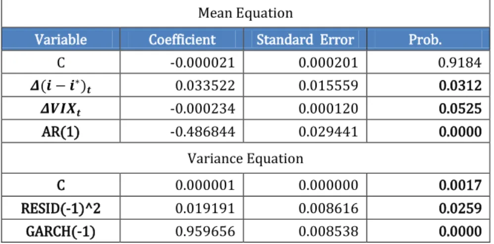
The ordinary least-squares regression revealed autocorrelation in the residuals as well as ARCH-effects. ARCH-effects in the residuals are a result of high volatility clustering, observ-able on the graph for daily changes in the spot exchange rate. Previous research findings sug-gest that ARCH effects are quite common when dealing with high-frequency data (Jansen & De Haan, 2005). A detailed description of statistical tests and graphical representation of the variables under consideration are listed in the Appendix under the corresponding section. To account for ARCH effects in the residuals, a GARCH(1,1) model is estimated. An auto-regressive term of order one, AR(1), is included in the mean equation to make sure there is no autocorrelation in the residuals. The first order of AR-term was chosen based on Akaike and Schwarz information criteria. The estimated output is provided in the table below.

Table 5-1-1: GARCH (1,1) estimated results.

Mean Equation

Variable Coefficient Standard Error Prob.

C -0.000021 0.000201 0.9184 ( ) 0.033522 0.015559 0.0312 -0.000234 0.000120 0.0525 AR(1) -0.486844 0.029441 0.0000 Variance Equation C 0.000001 0.000000 0.0017 RESID(-1)^2 0.019191 0.008616 0.0259 GARCH(-1) 0.959656 0.008538 0.0000

Source: Own calculations in Eviews.

In the table above all of the control variables are significant except for the constant term in the mean equation. Akaike and Schwarz information criteria as well as the value of are rather high for the model taken in first differences. A detailed description of the model statistics is listed in the Appendix. In addition to this, diagnostic checks were performed, which proved that the obtained results are robust. A normal probability plot is listed below.

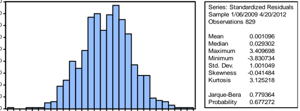
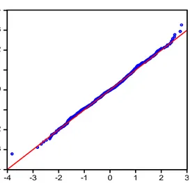
Figure 5-1-1: Normal probability plot of standardized residuals, GARCH(1,1) process.

By looking at the normal probability plot statistics, it is fairly obvious that normality assump-tions are satisfied. The estimated skewness indicator is insignificantly less than zero, while kurtosis coefficient is insignificantly different from 3. The value of Jarque-Bera statistic is equal to 0.7794 with a probability of 0.6773, which is well above the 5%-critical level. There-fore, the residuals are said to be normally distributed.

Consequently, in the next section the benchmark model will be estimated in first differences with the inclusion of event dummies. Dummy variables will enter the model in first differ-ences so that all variables in the model are integrated of order 1. An exponential GARCH model will be estimated to account for asymmetric responses of the spot exchange rate to credit rating news.

5.2

Reactions to Standard & Poor’s credit rating announcements

In accordance with the equation(15), discussed previously in the methodology section of this paper, a compressed version of the estimated equation takes the following form:

( )

,

where event dummies, , are divided into three categories to distinguish between actual rating downgrades, outlook and watch revisions.

The correlation matrix of independent variables revealed high correlation coefficient between rating downgrades and outlook revisions (see the corresponding section of the Appendix for a detailed representation.) As a matter of fact, outlook dummies were excluded from the model to avoid multicollinearity problems.

Based on Akaike and Schwarz information criteria, only 1-day lagged values of event dum-mies are included in the model. Higher order lags of event dumdum-mies, as well as, forward-looking values of dummy variables (which were used to test whether forex markets anticipat-ed cranticipat-edit rating events), were found to be statistically insignificant. The estimatanticipat-ed results are provided in the tables below. Statistically significant explanatory variables are highlighted for convenience of a reader. A more detailed description of the regression output is listed in the Appendix under the corresponding section.

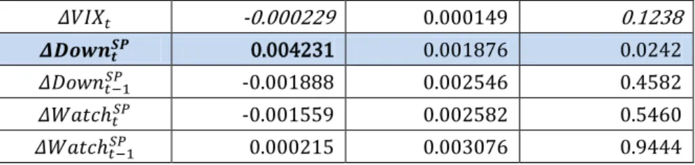
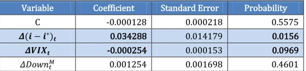
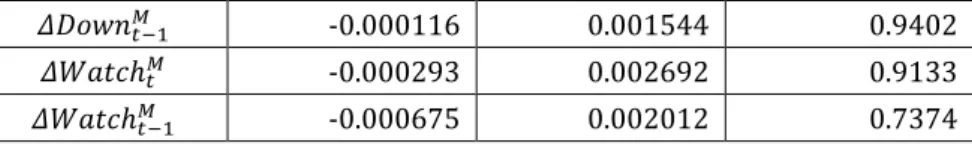
Table 5-2-1: Mean equation for exchange rate responses to S&P’s announcements.

Variable Coefficient Standard Error Probability

Constant -0.000147 0.000223 0.5102 ( ) 0.032612 0.014243 0.0220 0 10 20 30 40 50 60 70 80 90 -4 -3 -2 -1 0 1 2 3

Series: Standardized Residuals Sample 1/06/2009 4/20/2012 Observations 829 Mean 0.001096 Median 0.029302 Maximum 3.409698 Minimum -3.830734 Std. Dev. 1.001049 Skewness -0.041484 Kurtosis 3.125218 Jarque-Bera 0.779364 Probability 0.677272

-0.000229 0.000149 0.1238

_{0.004231 0.001876 0.0242}

-0.001888 0.002546 0.4582

_{-0.001559 0.002582 0.5460}

0.000215 0.003076 0.9444

Table 5-2-2: Variance equation for exchange rate responses to S&P’s announcements.

Variable Coefficient Standard Error Probability

ω (constant) -3.958062 1.702652 0.0201 α 0.189639 0.070680 0.0073 γ -0.059304 0.053327 0.2661 β 0.637537 0.159975 0.0001 ( ) 0.041382 0.063306 0.5133 0.013157 0.006210 0.0341 _{0.107743 0.489824 0.8259} 0.211099 0.516707 0.6829 _{-0.074169 0.508254 0.8840} -0.094016 0.507843 0.8531

Source: Own calculations in Eviews.

Interpretation

Mean equation

A change in interest differential, ( ) , is statistically significant at 95% confidence in-terval. The sign of the estimated coefficient is greater than zero, which is in line with the model assumptions, discussed earlier in the paper. A positive sign implies that 1% increase in the daily change of interest differential is associated with 3.26% Euro depreciation. Higher domestic interest rate (3-month EURIBOR) relative to the foreign interest rate (3-month US LIBOR) reflects higher inflation expectations, therefore, exports are expected to rise and val-ue of the domestic currency will fall, leading to a subseqval-uent Euro depreciation. High-interest currencies are believed to attract investors as there are potential gains from currency carry trades13. The behavior of investors that motivates their investment decisions, however, chang-es drastically during periods of financial distrchang-ess. Low-interchang-est currencichang-es, on the contrary, be-come more attractive to investors in situations of high uncertainty. This phenomenon is often referred to as “flight to quality”. As a matter of fact, demand for the US dollar was almost as high as during the pre-crisis period, owing mostly to its low interest rates. (Deutsche Bundesbank, 2010) Consequently, upward pressures on the US dollar drove the value of the Euro down, resulting in a substantial Euro depreciation against the US dollar.

Daily changes in the volatility index, , are only marginally significant (p=0.12). Thus, an increase in the volatility index, causes the Euro to appreciate (due to the negative

13 _{Currency carry trades refer to the situation when investors tend to borrow funds in low-interest-rate currency}

and invest them in higher interest-paying currency. Assuming that transaction costs are insignificant, thereby making an assumption that uncovered interest rate parity holds, potential benefits from carry trades will be equal to the interest rate differential ( (Brunnermeier, Nagel, & Pedersen, 2008), (Galati, Heath, & McGuire, 2007)).

cient) against the US dollar by 0.023%. A detailed interpretation of the following economic relationship between daily changes in the spot exchange rate and changes in the volatility in-dex will be discussed later on in the paper.

Of all event dummies, included in the mean equation, only downgrade announcements by S&P’s are found to be significant. Since the spot exchange rate EUR/USD enters the model in direct quotation (Euro per 1 USD), a positive sign of the corresponding coefficient implies that a downgrade announcement is associated with 0.42% Euro depreciation on the day of the announcement. This result is statistically significant at 95% confidence interval. This finding is in line with the assumptions of the model: negative credit rating announcements are ex-pected to drive down value of the domestic currency.

Variance equation

In the variance equation, β-coefficient is positive, which satisfies the model assumptions and non-negativity constraints. The coefficients of interest, however, are α and γ. The latter, which represents leverage effects between the mean and the variance of the spot exchange rate, is negative but insignificant. The α-coefficient is above zero and statistically significant at 1% significance level. With α being statistically significant while γ is not, the implication is as follows: the asymmetric impact of credit rating signals in not important, while the magnitude of credit rating announcements is.

The volatility index is, thus, the only regressor among explanatory variables, which is statisti-cally significant at 95% confidence interval. The volatility of the spot exchange rate increases by 1.32% when the volatility index, which represents an increase in global investor risk, rises by 1%. This result implies that even small volatility shocks in forex options market cause the variance of EUR/USD exchange rate to increase substantially.

Diagnostic tests

Figure 5-2-1: Q-Q plot of standardized residuals.

Diagnostic checks confirm that the estimated regression results are robust. There are no ARCH effects in the residuals. Normality conditions of a classical regression model are satis-fied. A visual representation of all diagnostic tests, performed on this model, is provided in the Appendix under a corresponding section. Since all points in the Q-Q plot, listed above, lie along the straight line, the residuals are said to be white noise.

-4 -3 -2 -1 0 1 2 3 4 -4 -3 -2 -1 0 1 2 3 Quantiles of RESID_GED_AR_1 Q u a n ti le s o f N o rm a l

5.3

Reactions to Fitch Rating’s credit rating announcements

In accordance with the equation(15), discussed previously in the methodology section of this paper, a compressed version of the estimated equation takes the following form:

( )

where event dummies, , are divided into three categories to distinguish between actual rating downgrades, outlook and watch revisions.

Since credit rating downgrades and outlook announcements are highly correlated as it is seen in the correlation matrix, provided in the Appendix, outlook announcements are excluded from the model.

Based on Akaike and Schwarz information criteria, only 1-day lagged values of event dum-mies are included in the model. Higher order lags of event dumdum-mies, as well as, forward-looking values of dummy variables (which were used to test whether forex markets anticipat-ed cranticipat-edit rating events), were found to be statistically insignificant. The estimatanticipat-ed results are provided in the tables below. Statistically significant explanatory variables are highlighted for convenience of a reader. A more detailed description of the regression output is listed in the Appendix under the corresponding section.

Table 5-3-1: Mean equation for exchange rate responses to Fitch’s announcements.

Variable Coefficient Standard Error Probability

Constant -0.000144 0.000218 0.5091 -0.000218 0.000146 0.1342 ( ) 0.032200 0.014349 0.0248 0.000564 0.001706 0.7410 0.001431 0.001469 0.3298 0.000584 0.002194 0.7901 0.003149 0.001576 0.0457

Table 5-3-2: Variance equation for exchange rate responses to Fitch’s announcements.

Variable Coefficient Standard Error Probability

ω (constant) -4.730256 1.444022 0.0011 α 0.184546 0.072248 0.0106 γ -0.032387 0.053286 0.5433 β 0.564955 0.135638 0.0000 0.016831 0.005784 0.0036 ( ) 0.075496 0.070578 0.2848 0.418265 0.404004 0.3005 -0.532523 0.500829 0.2877 -1.092102 0.947344 0.2490 -1.270290 0.791432 0.1085