Application of the Seismic Reflection Method in Mineral Exploration and Crustal Imaging: Contributions to Hardrock Seismic Imaging

(1)

ACTA UNIVERSITATIS

UPSALIENSIS

Digital Comprehensive Summaries of Uppsala Dissertations

from the Faculty of Science and Technology

1269

Application of the Seismic

Reflection Method in Mineral

Exploration and Crustal Imaging

Contributions to Hardrock Seismic Imaging

OMID AHMADI

ISSN 1651-6214 ISBN 978-91-554-9290-8

(2)

Dissertation presented at Uppsala University to be publicly examined in Hambergsalen, Geocentrum, Villavägen 16, Uppsala, Friday, 25 September 2015 at 10:00 for the degree of Doctor of Philosophy. The examination will be conducted in English. Faculty examiner: Dr. Gilles Bellefleur (Geological Survey of Canada).

Abstract

Ahmadi, O. 2015. Application of the Seismic Reflection Method in Mineral Exploration and Crustal Imaging. Contributions to Hardrock Seismic Imaging. Digital Comprehensive

Summaries of Uppsala Dissertations from the Faculty of Science and Technology 1269. 76 pp.

Uppsala: Acta Universitatis Upsaliensis. ISBN 978-91-554-9290-8.

The seismic reflection method has been used extensively in mineral exploration and for imaging crustal structures within hardrock environments. In this research the seismic reflection method has been used and studied to address problems associated with hardrock settings. Papers I and II, address delineating and imaging a sulfide ore body and its surrounding rocks and structures in Garpenberg, central Sweden, at an active mine. 3D ray-tracing and finite-difference modeling were performed and the results suggest that although the detection of the ore body by the seismic reflection method is possible in the area, the presence of backfilled stopes in the mine makes seismic imaging of it difficult. In paper III the deeper structures of the Pärvie fault system in northern Sweden were revealed down to about 8 km through 2D seismic reflection profiling. The resulting images were interpreted using microearthquake data as a constraint. Based on the interpretation, some locations were suggested for future scientific deep drilling into the fault system. In paper IV, the seismic signature of complex geological structures of the Cue-Weld Range area in Western Australia was studied using a portion of a deep 2D seismic reflection profile. The pronounced reflections on the seismic images were correlated to their corresponding rock units on an available surface geological map of the study area. 3D constant velocity ray-tracing was performed to constrain the interpretation. Furthermore, the proposed structural model was tested using a 2D acoustic finite-difference seismic modeling method. Based on this study, a new 3D structural model was proposed for the subsurface of the area. These studies have investigated the capability of the seismic reflection method for imaging crustal structures within challenging hardrock and complex geological settings and show some its potential, but also its limitations.

Keywords: Seismic reflection, Hardrock, Mineral exploration, Crustal imaging, Interpretation,

Modeling

Omid Ahmadi, Department of Earth Sciences, Geophysics, Villav. 16, Uppsala University, SE-75236 Uppsala, Sweden.

(3)

Dedication

(4)

(5)

List of Papers

This thesis is based on the following papers, which are referred to in the text by their Roman numerals.

I Ahmadi O, Juhlin C, Malehmir A, Munck M (2013) High-resolution

2D seismic imaging and forward modeling of a polymetallic sulfide deposit at Garpenberg, central Sweden. Geophysics 78:B339–B350. doi: 10.1190/geo2013-0098.1

II Ahmadi O, Juhlin C (2015) The effect of the backfilled stopes on

seismic imaging of a sulfide deposit in Garpenberg, central Sweden. Manuscript.

III Ahmadi O, Juhlin C, Ask M, Lund B (2015) Revealing the deeper

structure of the end-glacial Pärvie fault system in northern Sweden by seismic reflection profiling. Solid Earth 6:621–632. doi: 10.5194/se-6-621-2015

IV Ahmadi O, Koyi H, Juhlin C, Gessner K (2015) Seismic signatures

of complex geological structures in the Cue-Weld Range area, Mur-chison domain, Yilgarn Craton, Western Australia. Submitted to Tectonophysics.

The published papers were reprinted with the permission from the corre-sponding publishers. In addition, below is a list of other publications during my PhD studies, which are not included in the thesis:

Ahmadi O, Juhlin C, Gessner K (2014) New Insights from Seismic Imaging

Over the Youanmi Terrane, Yilgarn Craton,Western Australia. Energy Procedia 59:113–119. doi: 10.1016/j.egypro.2014.10.356

Ahmadi O, Hedin P, Malehmir A, Juhlin C (2013) 3D seismic interpretation

and forward modeling – an approach to providing reliable results from

2D seismic data. In: 12th Biennial SGA Meeting. Society for Geology

Applied to Mineral Deposits (SGA), Uppsala, Sweden.

Ahmadi O, Juhlin C (2013) Seismic Forward Modeling of a Poly-metallic

Massive sulfide Deposit at Garpenberg, central Sweden. In: 75th_EAGE

Conference & Exhibition incorporating SPE EUROPEC 2013. The Eu-ropean Association of Geoscientists and Engineers (EAGE), London, United Kingdom.

(6)

(7)

1. Introduction

Exploration seismology has been established since 1923 and it has been used extensively in natural resources exploration (Sheriff and Geldart 1995; Dentith and Mudge 2014). The basic idea behind it is that seismic waves travel through the earth and may be refracted, reflected or diffracted once they reach an inter-face with different seismic impedance properties compared to their surrounding rocks. The reflected or refracted seismic waves bring us very useful information about the rocks and geological structures in the subsurface. There are generally different methods in exploration seismology which can be implemented in order to address specific problems. One of the most commonly used method is the seismic reflection method (Sheriff and Geldart 1995; Yilmaz 2001) in which reflected or diffracted waves are studied (Telford et al. 1990; Sheriff and Geldart 1995). The geometry of the subsurface structures and their accurate delineation are of great interest to exploration geoscientists. Knowledge about geological structures may have different applications in various projects such as geotechni-cal invistigations, mine-planning, reservoir estimation, oil, gas and mineral ex-ploration (Malehmir et al. 2012a; Telford et al. 1990; Dentith and Mudge 2014). In mineral exploration, the seismic reflection method has had proven capability for almost six decades (e.g. Schmidt 1959; Wu et al. 1995; Eaton et al. 1996; Milkereit et al. 2000; Adam et al. 2003; Bohlen et al. 2003; Malehmir et al. 2012a). The strength of the method lies in its good signal penetration, which makes the method capable of imaging deep targets and structures (e.g. Malehmir et al. 2012a and references therein). This benefit led the mining industry to take advantage of the method and seek solutions to their prospecting problems with the seismic reflection method (Malehmir et al. 2012a). Apart from its applica-tion in natural resource exploraapplica-tion, the seismic reflecapplica-tion method may be used to image crustal structures (e.g. Lie and Andersson 1998; Juhojuntti et al. 2001; Hobbs et al. 2006; Martínez Poyatos et al. 2012). Understanding the geometry of crustal structures is important and may have applications in risk assessment of natural hazards such as earthquakes, studies of geodynamical processes and detecting mineral deposits associated with geological structures (e.g. Williams et al. 1995; Hurich 1996; Larkin et al. 1996; Haugen and Schoenberg 2000; Juhlin et al. 2000; Juhojuntti et al. 2001; Hobbs et al. 2006; Goleby et al. 2006; Ji and Long 2006; Juhlin et al. 2010; Campbell et al. 2010; Juhlin and Lund 2011; Cheraghi et al. 2011; Lundberg et al. 2012; Ehsan et al. 2014; Jackson et al. 2015). In this thesis, three main problems have been addressed using the seismic reflection method. The first problem is delineating a sulfide deposit at an active

(12)

mine in central Sweden. The second is revealing the deeper structure of an end-glacial fault system in northern Sweden, and the third is an interpretation of a 2D seismic reflection profile through a complex geological setting in Western Aus-tralia. All these case studies are located within crystalline or hardrock environ-ments. Seismic imaging in hardrock settings is challenging and has been ad-dressed by many researchers around the world (e.g. Nelson 1984; Harman et al. 1987; Read 1989; Milkereit et al. 2000; Adam et al. 2003; Bohlen et al. 2003; Nedimovic and West 2003; Salisbury et al. 2003; Li and Eaton 2005; Dehghannejad et al. 2010; Bongajum et al. 2012; Malehmir et al. 2012a; Greenhalgh and Manukyan 2013; Bellefleur et al. 2015; Buske et al. 2015; Koivisto et al. 2015; Manzi et al. 2015). This dissertation is a comprehensive summary of four papers and consists of four chapters. In the first chapter, an introduction and background of the study is given. The second chapter deals with a definition of the hardrock environment. I have tried to summerize all the methods that I have used in chapter 3, including numerical and experimental methods. Finally, in chapter 4, all the papers upon which the thesis is based on, are summarized.

In paper I, the seismic reflection method was used in attempt to delineate and enhance the image of a sulfide ore body and its surrounding rocks and structures in Garpenberg, central Sweden. A high resolution 2D seismic reflection profile was acquired at an active mine site, a challenging and noisy environment. The seismic data were processed along a straight CDP line and an interpretation was made based on the migrated section. 3D ray-tracing modeling was performed to test the interpretation. A few rock samples from the ore body were provided by Boliden Mines and these were used to estimate the P-wave velocity of the sul-fide ore.

In paper II, I expanded the research by including the backfilled stopes in the modeling that had been mined out and refilled during the mining process. Addi-tional rock samples were collected from the mine and their physical properties measured using an ultrasonic instrument. In order to obtain more reliable results and a better approximation to the wave equation, a 3D acoustic finite-difference method was used for modeling.

In paper III, the deep structures of the Pärvie fault system were revealed down to about 8 km via a new 2D seismic profile. Furthermore, an interpretation was made using microearthquake data as a constraint. Based on the interpreta-tion, some locations were suggested for future scientific deep drilling into the fault system.

In paper IV, the seismic signature of the complex geology of the Cue-Weld Range area in Western Australia was studied. Enhanced structures on a 2D seismic section were correlated to their corresponding rock units on a surface geological map. 3D constant velocity ray-tracing was performed to constrain the interpretation. Furthermore, the interpretation was tested using a 2D acoustic FD method.

(13)

2. Hardrock environments

Rocks can be divided into three main groups: i) sedimentary rocks, ii) igne-ous rocks and iii) metamorphic rocks. Hardrock is a common term that is used for both igneous and metamorphic rocks while for sedimentary rocks, softrock is frequently used (Hall 1988). In general, hardrocks (e.g. granite, gneiss, quartzite) may be harder than sedimentary rocks (e.g. limestone, shale). Although this is true in the broad sense, there are some cases, which do not follow this rule. For instance, marble and limestone are classified as a hardrock and softrock respectively. But the calcite in limestone is as hard as that in marble. Moreover, the quartz grains in sandstone, which is a sedima-trary rock, are as hard as those in quartzite, a metamorphic rock. In addition, the quartz in sandstone which is classified as a softrock is harder than the calcite mineral in marble or even the feldspar or mica grains in granitic rocks (Hall 1988).

Hardrocks and softrocks may be found together in one place, but their origins will be quite different. The formation of hardrocks is controlled by magma flow, deformations, metamorphic and chemical processes in their localities while the deposition of sedimentary rocks is governed by surface or near-surface processes (such as precipitation, morphological processes, weathering etc.). Hardrock environments are often an assembly of complex structures which are formed during ductile and/or brittle deformations and magma emplacement (e.g. Van Kranendonk and Ivanic 2009). Hardrocks often have irregular spatial extent and appear in rough shapes, unlike the sedimentary rocks which commonly have regular dip and bedding. Addi-tionaly, hardrock terrains are also characterized with more discontinuities and greater heterogeneities (e.g. L’Heureux et al. 2009).

A variety of mineral deposits are hosted within hardrock settings. For ex-ample, volcanogenic massive sulfide deposits (VMS) are associated with extrusive igneous processes within intra- and inter-continental formation. Both supergene and hypogene processes may form iron ore bodies associ-ated with banded iron-formations (BIF) and gabbroic rocks (Robb 2005; Allen et al. 2008; Duuring and Hagemann 2013a). There are many other deposits which can be associated with hardrocks (e.g. Au, Cu-Ni, PGE, U and etc.).

In this thesis, three hardrock terrains will be discussed; i) the Lappberget sulfide ore body in central Sweden, ii) the end-glacial Pärvie fault system

(14)

within Paleoproterozoic greenstones in northern Sweden, and iii) the Cue-Weld Range, a neoarchean greenstone unit in Western Australia.

2.1. Lappberget sulfide ore body

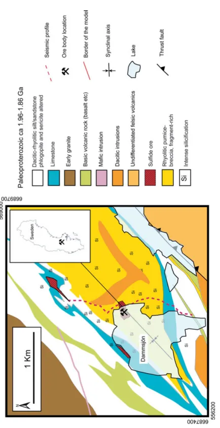
The Lappberget sulfide ore is an ore body within the Garpenberg deposit which is located in one of the most important mining regions of Sweden, known as Bergslagen (Stephens et al. 2009) (see Fig. 2.1). The region is well-known for hosting over 6000 mineral occurrences and has a long histo-ry of mining. Bergslagen formed during the Svecokarelian orogeny and is a part of the Fennoscandian Shield (Jansson 2011). Several stages of ductile-brittle deformation have affected the rocks in the region. The majority of the mineral deposits, including the Garpenberg deposit, are found within supracrustal volcanic inliers (Allen et al. 2008). The sulfide mineralogy of the Lappberget ore body consists of sphalerite (ZnS), galena (PbS), pyrite (FeS2) and lesser pyrrhotite (FeS), tetrahedrite ((Cu,Fe)12Sb4S13), argentite

(Ag2S) and alabandite (MnS). The ore body is located inside a domal

struc-ture in the central parts of the Garpenberg Syncline within an altered dacitic-rhyolitic rock unit (volcanic ash-siltstone). Figure 2.1 shows a geological map of the Garpenberg area.

2.2. The end-glacial Pärvie fault system

The Pärvie fault is located in the intraplate Baltic Shield, mostly composed of Paleoproterozoic rocks on the boundary to the Archean terrain of north-ernmost Sweden. The general strike of these rocks is parallel with, and only some 10-50 km away from the Ordovician Caledonian mountain front. Rock types range from acidic volcanic to ultrabasic intrusive rocks. Granitic rocks are extensively exposed at the surface (Fig. 2.2). In some places, sedimen-tary rocks such as sandstone and limestone crop out. The establishment of permanent seismic stations in northern Sweden in 2003-2004, as part of the Swedish National Seismic Network (Bödvarsson and Lund 2003), showed that the Pärvie fault, and the other end-glacial faults in northernmost Swe-den, are still seismically active. Lindblom et al. (2015) analyzed the earth-quakes recorded along the Pärvie fault between 2003 and 2013. Their study showed that the earthquakes occur all along the mapped fault scarp, mostly on the eastern side of the fault in accordance with an east-dipping reverse fault (Lindblom et al. 2015). At four locations along the main Pärvie fault recent investigations on outcrop scale provide the kinematics of brittle de-formation structures and identification of four paleostress fields. Three of the paleostress fields are also found in other major shear zones in the area (Edfelt et al. 2006), whereas the fourth, and most recent field, seems to be

(15)

unique for the Pärvie fault. This structure indicates a reverse stress field with a strike-slip component. Figure 2.2 shows a geological map of the Pärvie area.

2.3. Cue-Weld Range greenstone unit

The Weld Range area is located about 60 km NNW of the town of Cue in the northwestern part of Murchison domain which forms a granite-greenstone unit of the Youanmi terrane within the neoarchean Yilgarn carton in Western Australia (Fig. 2.3). The greenstones in the area have been divided into three major groups (Van Kranendonk and Ivanic 2009): i) mafic volcanic rocks, felsic volcaniclastic sandstones and BIF of the Norie group, 2825-2800 Ma ii) the Polelle group of mafic volcanic rocks, felsic volcanic and volcaniclastic sedimentary rocks and banded iron-formation (BIF) with an age of 2785-2800 Ma and iii) the Glen group of coarse clastic sedimentary rocks and komatiitic basalt, 2724-2700 Ma (Figure 2.3). Voluminous granit-ic rocks were emplaced extensively from 2716 to 2592 Ma. Supercrustal rocks in the area have been metamorphosed to lower greenschist facies (Duuring et al. 2012). The two deformation phases that control geological relationships in the area are: 1) the D1 deformation, which produced the E-trending folds and occurred at the same time as granitic rock emplacement at about 2676 Ma, 2) the regional D2 shortening in the east-west direction which formed the N- to NNE-trending folds from 2660 to 2637 Ma. The second deformation (D2) produced foliation and lineation in the supercustal rocks as well as NNW-striking sinistral shear zones and NE-striking dextral shear zones in the area (Duuring and Hagemann 2013a). The main iron de-posits are hosted within the gabbroic complex of the Weld Range area and there is a high demand to mine them out.

(16)

Fi gu re 2. 1. B edr oc k geol ogi ca l m ap o f t he Gar pe nbe rg ar ea (m odi fi ed af te r Al le n et al . 20 03 ). T he i ns et m ap sh ow s t he l ocat io n of t he a rea in Swe den. T he dashe d line s

hows the seism

ic pr ofi le ove r th e Lap pb er get o re bo dy .

(17)

Fi gu re 2. 2. B edr oc k geol ogy of th e Pär vi e ar ea in no rt he rn Swe den ( © Lant m äter iet I 201 4/0 06 01) .Th e inse t m ap sh ows th e lo cation o f th e area in Swed en . The b lack lin e sho w s th e lo cation o f th e seism ic profile.

(18)

Fi gu re 2. 3. Ge ol og ical m ap o f t he C ue -W el d R ange area (I vani c et al. 2013 b). Th e in set sh ows th e l ocatio n of th e area in Wester n Australia.

(19)

3. Methods

In order to address the problems in all the case studies I have been involved in I used the 2D seismic reflection method. The success of the method in hardrock enviroments has been proven by many reported studies around the world (e.g. Wu et al. 1995; Wu et al. 1995; Eaton et al. 1996; Milkereit et al. 2000; Juhlin et al. 2000; Adam et al. 2003; Bohlen et al. 2003; Nedimovic and West 2003; Dehghannejad et al. 2010; Manzi et al. 2012; Harrison and Urosevic 2012; Malinowski et al. 2012; White et al. 2012; Bellefleur et al. 2012; Malehmir et al. 2013; Bellefleur et al. 2015; Cheraghi et al. 2015). I processed three seismic data sets and imaged subsurface structures of each area along corresponding 2D seismic profiles. In the Lappberget case study, some samples from the target ore and surrounding host rock were collected. This allowed me to measure and obtain physical properties of the samples using an ultrasonic system. In the first paper, in order to provide more con-straints for the interpretation of the seismic data, 3D ray-tracing was per-formed. Later, to improve the modeling, 3D finite difference modeling was carried out in the second paper. In the third paper, a seismic reflection profile was processed to delineate the geometry of the Pärvie fault system. In the fourth paper, I performed 2D acoustic finite-difference modeling and a 3D constant velocity ray-tracing. In the following sections, I briefly explain each method that I used throughout my research.

3.1. Seismic reflection method

The seismic reflection method is sensitive to the seismic impedance contrast of the rocks through which the waves propagate. In general, a reflection form a structure may be observed if there is a significant impedance contrast between the structure and the surrounding media. In addition, the signal-to-noise ratio of the seismic data and the fold are other important factors in seismic imaging. Normally, the seismic reflection method is carried out in two phases; seismic data acquisition, and then seismic data processing. These are discussed in the following sections.

(20)

3.1.1. Seismic data acquisition

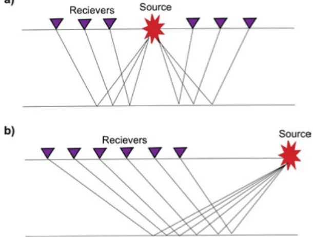
Enhancing a clear reflection originating from a geological structure, requires sorting source gathers into a set of gathers in which their seismic traces have a common midpoint (CMP). These gathers are named CMP or CDP (com-mon depth point) gathers and the number of traces within each CDP gather equals the fold of that gather. In order to achieve enough fold-coverage for imaging, each reflecting point must be recorded more than once (Sheriff and Geldart 1995). In CMP or CDP recording a seismic spread should move continuously down the seismic line to record and obtain the desired fold-coverage. There are a number of seismic spread types that can be used (Sher-iff and Geldart 1995). Out of these, three of them were employed to acquire the data used in the papers: i) fixed-spread ii) split-spread and iii) end-on spread.

In the fixed-spread the receiver line is fixed and the source moves along the seismic profile. This type of spread is suitable when the length of the profile is relatively short. Moving the source results in a good fold coverage. In paper I, an example of a fixed-spread is demonstrated.

Split-spread is a common survey type where the source is located in the center of the receiver line (Fig. 3.1a). Receivers are spaced regularly depend-ing upon the desired lateral resolution. For example, in a deep seismic sur-vey, 40 m group geophone spacing can be used (see paper IV). Another common seismic survey type is the end-on spread. In the end-on configura-tion, the source is located at one end of the receiver line (Sheriff and Geldart 1995) and receivers are spaced regularly (Fig. 3.1b).

Figure 3.1.Two types of seismic spreads: a) split-spread and b) end-on spread.

Seismic data acquisition may be acquired along a straight or crooked line and, depending on which, the seismic data may be processed in different

(21)

ways. The apparent dip of the structures may change if the direction of the seismic line changes. Therefore to avoid ambiguity during interpretation, there should be an effort to design straight seismic lines as much as possible (Sheriff and Geldart 1995). However, in practice this is not always possible because of access and structural complications, especially in hardrock envi-ronments which are usually ruggy and difficult terrains. Therefore, most seismic data are acquired along crooked lines.

3.1.2. Seismic data processing

In the seismic reflection method, we aim to image subsurface structures or singularities. In the conventional seismic data processing, the imaged struc-tures in the final seismic section should be migrated to their true locations at depth. Most migration algorithms are based on the single-diffracting as-sumption, while in fact seismic waves are multiple diffracted in the presence of random noise in the medium when propagating through the heterogeneous subsurface (Fleury 2012; Broggini and Snieder 2012). This implies that seismic data should be processed to provide the data ideally free of noise, multiples and unwanted wave modes (e.g. S-waves, ground roll and surface waves) before migration. In general, conventional seismic data proceesing can be divided into three main steps: 1) deconvolution 2) CDP stacking and 3) migration (Yilmaz 2001). In addition, there are some other common proc-essing operations that should be applied before the main procedures. Pre-processing, noise attenuation and filtering, static corrections and cross-dip correction are some of these. Before explaining the main processing steps, the preprocessing operations are briefly summarized.

Pre-processing is required to convert the format of the seismic data. Usu-ally, the data are acquired in SEGD format and in order to process it, the data need to be converted to SEGY format, which is a standard format for seismic data processing (Sheriff and Geldart 1995; Dentith and Mudge 2014). The geometry of the seismic line should be set up. Accurate coordinates of source and receivers must be defined since these play an important role in static corrections and stacking of the data correctly.

Filtering is an essential step in seismic data processing. In order to re-move or attenuate unwanted waveforms such as ground roll and airwaves, an appropriate filter can be designed and applied to the data. For example a high-pass filter may be applied to remove low-frequency surface waves (Dentith and Mudge 2014). Dip-filtering (f-k filtering) can also be used if carefully designed. Sometimes, because of the complexity of the subsurface, it is not straightforward to obtain a clean shot gather with only one filter. Therefore, we may need to design and apply a time-varing filter and enhance reflections appropriately at different arrival times.

(22)

Static corrections have a great effect on boosting refletions. These correc-tions are divided into two groups: i) refraction static correccorrec-tions ii) reflection (residual) corrections (Yilmaz 2001). The refraction static corrections try to correct for near surface low velocities. These low velocities correspond to weathered or the loose sediments near the surface and may cause local varia-tions in arrival times (Dentith and Mudge 2014). Therefore, we need to ap-ply a time shift to restore the seismic traces as if they were recorded in an ideal terrain with constant topographic elevation (Dentith and Mudge 2014). Furthermore, we may apply reflection (residual) static corrections where a time shift based on the lateral coherceny of the reflections is calculated and applied to increase coherency of the reflections in the seismic data (Dentith and Mudge 2014).

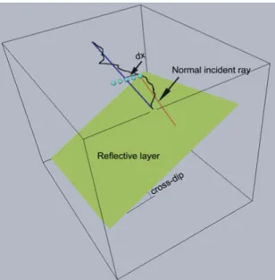
The cross-dip correction is necessary to correct for out-of-plane compo-nents or reflections in the seismic data (Sheriff and Geldart 1995). This cor-rection is more relevant when the seismic line is crooked (see Figure 3.2) (Larner et al. 1979; Nedimovic and West 2003; Rodriguez-Tablante et al. 2007). The procedure consists of applying calculated cross-dip corrections on normal moveout (NMO)-corrected CDP-binned gathers and then stacking the CDP gathers. Equation (3.1) expresses the calculation of the cross-dip correction where dx is the perpendicular distance of a midpoint from the stacking line:

. (3.1)

(23)

Figure 3.2. A crooked seismic line (black line) and a layer with a cross-dip compo-nent. Cross-dip corrections can be calculated by equation (3.1) for this layer. The blue line depicts the CDP stacking line.

3.2.1.1. Deconvolution

Ideally, we would like to extract the earth’s reflectivity from seismograms. In order to do this, deconvolution can be applied. Deconvolution tries to sharpen the wavelet using an inverse filter and thus increase temporal resolu-tion of the data (Yilmaz 2001). In theory, convolving the deconvoluresolu-tion op-erator with the seismic trace results in a series of spikes which represent the subsurface reflectivity. In this concept, it is assumed that the seismic wavelet is a minimum-phase wavelet and therefore the source wavelet is already known. This type of deconvolution is called spiking deconvoltion (Yilmaz 2001). But in practice, because of the complexity of the surface, the source wavelet may vary during the seismic recording. In this case, predictive de-convoltion can be used. In this type of deconvolution, an effort is needed to to design a reasonable inverse operator (Yilmaz 2001) by changing different parameters (such as gap, length and random noise level).

3.2.1.2. CDP stacking

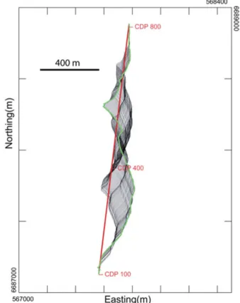
Stacking along a CDP line is another complimentary procedure which will normally attenuate noise and multiples (Yilmaz 2001). In order to design a CDP line, coordinates of receivers and sources must be defined accurately. A desired CDP line needs to be defined depending upon the geometry of the seismic profile (Fig. 3.3). If the line is crooked, then it is best to split the CDP line into a number of straight segments which run within mid-points

(24)

(Wu 1996). CDP bins are usually designed perpendicular to the CDP line, but can also be at some angle to the stacking line where the CDP bins are parallel to strike of the geological structures (Kashubin and Juhlin 2010; Lundberg and Juhlin 2011). The seismic data are then sorted in CDP gathers.

Figure 3.3. Straight CDP line (red line) along the 2D cooked seismic profile (green line) in Garpenberg, Sweden (Paper I). The black cloud depicts mid-points of the seismic data.

Since conventional seismic imaging and migration is based on zero-offset traces, it is necessary to correct the seismic traces to as if they had been ac-quired with the sources and receives at the same location (zero-offset). The normal moveout correction (NMO) is the simplest correction that can be made to obtain the zero-offset traces (Yilmaz 2001). A drawback of the NMO correction is that it does not take into account confilicting dips in the subsurface and therefore a bias arises in achieving good zero-offset gathers (Yilmaz 2001). Additionaly, the moveout of steeply-dipping layers is in con-flict with the moveout associated with gently-dipping structures (Yilmaz 2001). In order to enhance possible dipping layers, dip moveout (DMO) is another pre-stack process which may be applied (Hale 1984; Deregowski 1991). After applying DMO, the NMO correction should follow and the

(25)

resulting zero-offset CDP gathers be stacked to provide a final stacked sec-tion in the time domain.

3.2.1.3. Migration

Migration is the final process applied to re-position reflections to their true geological positions at depth (Yilmaz 2001). Migration also collapses dif-fractions and improves the quality of the final image (Yilmaz 2001). In con-ventional seismic data processing, migration is applied after stacking and is called post-stack migration, while it may be applied on pre-stack data as well (pre-stack migration). The accuracy of the final migrated section highly de-pends on the input velocity model (Jones 2010). Hence, a great effort should be made to obtain a good velocity model, which is a major challenge in complex and hardrock environments. Based on the type of algorithm, migra-tion methods can be divided into two major groups: 1) ray-based migramigra-tion methods and 2) differential equation-based migration methods (Jones 2010). Kirchhoff migration is a common ray-based (integral) method which can be applied even when steeply-diping layers are present (Yilmaz 2001). A draw-back of this method is the difficulty to handle lateral velocity variations (Yilmaz 2001). Differential equation-based methods can be divided into two subgroups: 1) finite-difference (FD) based methods (e.g. downward con-tinuation or FD method) and 2) frequency-wave number based methods (e.g. Stolt method) (Yilmaz 2001). The FD method handles well any type of sub-surface velocity model, but one needs to be very careful on choosing the right dip approximation for the method (Yilmaz 2001). In contrast, the fre-quency-wave number methods are limited in handling lateral velocity varia-tions (Yilmaz 2001). Therefore, each migration method has its own advan-tages and drawbacks and the selection of the method to be used is case de-pendent.

3.2. Interpretation and forward modeling

Final migrated seismic sections should be interpreted and all imaged struc-tures should, when possible, be correlated to mapped rock units on surface geological maps or stratigaphical columns extracted from well logs. Occa-sionally, there is a lack of information and it is not possible to interpret re-flections with confidence. However, even with few constraints, it is still fea-sible to provide an explanation for prominent reflections. Forward modeling has an important role to evaluate and test interpretations. A synthetic data can be produced with the same survey configuration as the real data. The real and synthetic data can then be compared (e.g. Blake et al. 1999; Bohlen et al. 2003; L’Heureux et al. 2009; Cheraghi et al. 2011; Malinowski et al. 2012; Bellefleur et al. 2012; Squelch et al. 2013). In practice, interpreted structures and their corresponding physical properties can be discretized on

(26)

1D, 2D or 3D grids. Furthermore, a numerical experiment can be performed throughout the grid and simulate wave propagation with the same survey as the real layout. There are many methods to model seismic wave propagation. Ray-tracing and finite-difference methods are the most common techniques that I have also used in the course of my research.

3.2.1. Ray-tracing

Asymptotic ray-tracing is a high frequency based technique to simulate seismic rays and calculate arrival times for the modeled reflections. In order to avoid the scattering problem with long wavelength seismic waves, we need to use the high frequency approximation to the wave equation (Gjøystdal et al. 2002; Chapman 2004). By employing the ray-tracing tech-nique, we aim to calculate traveltimes to reflectors in a model. The ampli-tude of the reflections can also be calculated (Cerveny 2005). The essential governing equations of the method for acoustic media are briefly presented here. Acoustic wave propagation through a smoothed inhomogeneous media can be represented with the following equation (Cerveny 2005):

, (3.2)

where ϕ is the pressure wavefield, ϕtt is the second derivative of the

pres-sure field with respect to time and c(xi) is variable velocity function with

constant density assumed throughout the medium. The source term is not shown in the equation. The following time-harmonic high frequency solution satisfies the above equation:

, . (3.3)

Here is the high frequency term, while P(xi) and T(xi) are assumed to be smooth scalar functions of coordinates. Equation (3.3) forms a plane wave solution and plugging it into the equation (3.2) yields:

1

2 .

0. (3.4)

In order for equation (3.4) to be valid, we arrive at the Eikonal equation:

(27)

and the transport equation:

2 . 0. (3.6)

Equations (3.5) and (3.6) are very important and should be solved in the ray-tracing (Cerveny 2005). The last term∇ 2_{P in equation (3.4) also contains}

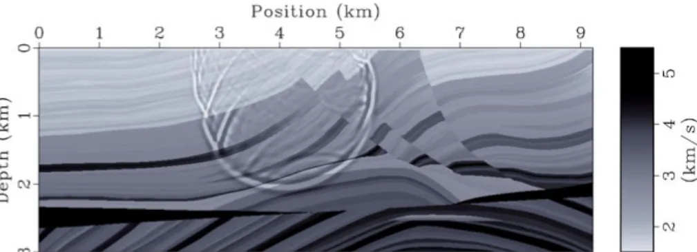
the amplitude of the waves and needs to be considered in some cases (Scales 1997). This amplitude term, may be written as a function in a series of in-verse powers of frequency and then can be solved for (Cerveny 2005). Fig-ure 3.4 shows the Marmousi model in which a source at 4 km distance is excited. The corresponding seismic rays are traced and overlaid on the model. Ray-trace modeling has been widely used around the world (e.g. Julian and Gubbins 1977; Cerveny 1989; Farra 1993; Blake et al. 1999; Gjøystdal et al. 2002). The governing equations can be expanded for more complex and heterogeneous media. In addition, elastic waves can also be considered (Cerveny 2005).

Figure 3.4. Ray-tracing through the Marmousi model. A seismic source is located at 4 km distance and at the top of the model (sea surface). The ray-tracing was per-formed using the CREWES toolbox in Matlab (Margrave 2000).

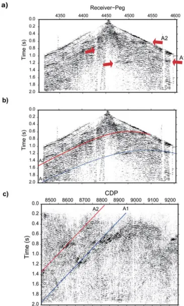
A simplified type of ray-tracing is 3D constant velocity ray-tracing, which was used in paper IV. This type of ray-tracing is suitable to model reflec-tions in pre-stack data and then track them on an unmigrated stacked section (Ayarza et al. 2000; Lundberg et al. 2012). The method is based on Fermat’s principle for traveltime calculations and the amplitude of the reflections can be calculated using the formulas given by Aki and Richards (2009). Using constant velocity ray-tracing, traveltime curves of planar reflections are cal-culated (Fig. 3.5). Dip and azimuth of a planar reflector are changed with an iterative approach in small increments until the best fit is achieved. Use of this method should result in the calculation of reasonable traveltimes for the reflections when velocity variations are small (Lundberg et al. 2012).

(28)

Figure 3.5. Calculated traveltimes using 3D constant velocity ray-tracing on a shot gather of the 10GA-YU1 data set in the Cue-Weld Range area, Western Australia: a) two reflections are prominent in the shot gather where reflection A1 appears to come to the surface while reflection A2 does not; b) travel times to a plane with a strike of N45°E and a dip of 30° NW match well with both reflections A1 and A2 and c) travel times of the modeled reflections on the unmigrated stacked section.

3.2.2. Finite-difference method

The finite-difference method is the most frequently used method for model-ing of seismic wave propagation (Fichtner 2011). This method provides a good approximation to the solution of the wave equation and it has been used for seismic modeling through various hardrock environments (e.g.

(29)

Yerneni et al. 2002; Bohlen et al. 2003; Saenger and Bohlen 2004; L’Heureux et al. 2009; Cheraghi et al. 2011; Bellefleur et al. 2012; Squelch et al. 2013). The wave equation has two general modes; the acoustic wave and elastic wave equations. The earth is an imperfect elastic media and the acoustic wave equation is only truly valid in a fluid media where the shear moduls equals zero (Aki and Richards 2009; Fichtner 2011). Therefore, in order to simulate wave propagation through the subsurface, it is preferable to use visco-elastic or elastic wave equations (Juhlin 1995; Saenger and Bohlen 2004). However, the acoustic wave equation is computationally less expen-sive than the elastic wave equation (Fichtner 2011). Using the acoustic mode of the wave equation is strictly only justifiable when the data processing is limited to the first arrivals of P-waves and also when an active seismic source (such as explosive) is used during recording that generates less S-wave energy (Fichtner 2011). However, the acoustic expression of the S-wave equation has been used extensively in active source seismic modeling (Alkhalifah 2000; Wang and Liu 2007; Sava and Poliannikov 2008; Bean and Martini 2010; Sava and Vlad 2011; Squelch et al. 2013). In this thesis, 2D and 3D acoustic FD methods were used. To understand the methods bet-ter, the mathematics of the 2D FD method is demonstrated below.

Equation (3.2) for a 2D acoustic problem may be expressed as follows: , ,

, , , . (3.7)

Now, the right side of the above equation can be written using the second order finite-difference approximation in the following form:

, ,

,

, , Δ

2 , , , , Δ ,(3.8)

and then we have:

, , Δ = 2 Δ , , ,

, , Δ . (3.9)

Based on equation (3.9), we are able to calculate the seismic wavefield at t+∆t using two earlier wavefields at t and t-∆t (Margrave 2003) (see Fig. 3.6).

The numerical experiment has to be stable and accurate as much as possi-ble. Spatial sampling (grid spacing) must be chosen adequately to avoid grid dispersion. The grid spacing (h) needs to satisfy the following general condi-tion, in order to have an accurate experiment and be as free of grid disper-sion as possible:

(30)

, (3.10)

where is the minimum wavelength in the model and n depends on

the order and length of the FD operator (Bohlen et al. 2015). For the 4th

-order in space and 2nd_{-order in time approximation we have (Bohlen et al.}

2003):

. (3.11)

If the amplitude of the solution grows without bound during the simula-tion, then the experiment is not stable. In order to avoid this, time-stepping ∆ should also fulfil the following condition (Fichtner 2011):

Δ , (3.12)

in which, and denote the minimum grid spacing and maximum

velocity in the model. The constant coefficient depends on the method used for space and time discretisation (Fichtner 2011). For example, for a

finite-difference algorithm based on the 4th_{-order and 2}nd_{-order approximation in}

space and time, respectively, and in a staggered grid, the expression (3.11) can be represented as (Blanch 1996; Bohlen et al. 2003):

Δ

√ , (3.13)

with d as the dimension of the model.

Figure 3.6. A snapshot of P-wave propagation through the Marmousi model at 1 s. The source is located at 4 km distance and at the sea surface. The FD modeling was performed using Madagascar software (Fomel et al. 2013).

(31)

The grid model used to discretize the subsurface physical properties is limited by boundaries. Therefore, during seismic modeling, reflections from the boundaries interfere with responses from structures within the model. This effect needs to be removed or attenuated. One way to do this is by add-ing a number of zero nodes to the boundaries to absorb the seismic energy (Fichtner 2011). Although the grid padding technique is not a perfect solu-tion for the boundary problem, it has been used widely (e.g. Juhlin 1995; Bohlen 2002; Margrave 2003; Fichtner 2011). However, this technique will not attenuate all seismic waves with arbitrary incident angles (Fichtner 2011). Furthermore, using the grid padding, makes the model bigger and therefore computationally more expensive. Fortunately, seismic modeling can be coded in parallel and be performed on cluster or multi-node comput-ers within a reasonable computational time (Bohlen 2002; Weiss and Shragge 2013; Fomel et al. 2013).

3.3. Measurements of acoustic properties

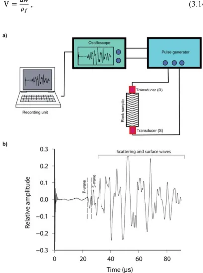
In order to carry out seismic modeling using either ray-tracing or FD meth-ods, we need to define the physical properties (velocities and densities) of the rocks as input. One way to do this is to collect some rock samples from the area of interest. The samples should represent the lithology range within the area as much as possible. Seismic velocities of the samples can be meas-ured using ultrasonic instruments (Vanorio et al. 2002; Salisbury et al. 2003; Stanchits et al. 2006; Malehmir et al. 2013). An ultrasonic device consists of two transducers (one receiver and the other source) connected to a pulse generator. The transducers induce a high frequency signal (e.g. 1 MHz) through the rock sample. A signal is passed through an oscilloscope and finally a computer to record the waveform (Fig. 3.7). The procedure can be done both at room condition and/or at elevated confining pressures (Salis-bury et al. 2003; Malehmir et al. 2013). The rock samples should be cut in a way to make flat surfaces on each side of the samples. Sometimes samples are taken from core where it is easy to cut the top and the bottom of the sam-ple. If the sample has an irregular shape, an effort should be made to form a cubic shape out of the sample (Malehmir et al. 2013). After cutting, the sam-ples are ready for the ultrasonic measurements. I performed the measure-ments at atmospheric condition due to the instrumental limitations.

The density of the rock samples should also be measured. Although the rock samples are cut for the ultrasonic measurements, they still appear with ir-regular shapes and the calculation of their densities is not straightforward. There are different methods to obtain the density values such as suspension, level and overflow methods (Hughes 2005).

(32)

Among these, the suspension method is the most accurate and precise method (Hughes 2005). This method is based on Archimedes’ principle. This principle states that when an object is suspended in a liquid, it displaces the liquid and the weight of the displaced liquid equals the force which buoyes up the object (Halliday et al. 2000). The suspension device consists of an electronic scale and a container with enough water to suspend the rock samples entirely in it (Fig. 3.8). Based on Archimedes’ principle, the volume of the immersed sample equals the difference in weight divided by the den-sity of the fluid (Hughes 2005):

V , (3.14)

Figure 3.7. Ultrasonic measurement: a) an illustration of the ultrasonic apparatus at room conditions; b) a recorded waveform through a sulfide ore sample from the Lappberget ore body using the ultrasonic instrument at room conditions.

(33)

where V is the volume of the sample, ∆w the difference in weight and ρf is the density of the fluid. If we use pure water as the fluid in the experiment with a density of about 1 (kg/m3_{), we can write:}

V

Δ . (3.15)

Figure 3.8. Density measurement based on Archimedes' principle using the suspen-sion device.

The mass of the sample can be measured using the electronic scale. We are then able to calculate the density of the sample as:

(34)

4. Summary of the papers

In this section, each paper is summarized to provide a brief description about the main goals, methods and results of the studies. My contributions in these studies were as follows:

Paper I: I participated in the data acquisition in 2011. I processed the

seis-mic data with advice from my supervisor. Boliden Mines provided the rock samples from the mine and I conducted the lab measurements using the ul-trasonic instrument. I performed the 3D ray-tracing using the Norsar-3D program (www.norsar.no/seismod/Products/NORSAR-3D/). The paper was written initially by me and later improved by my co-authors.

Paper II: I performed the numerical modeling using Madagasacr software

(www.ahay.org/wiki/Main_Page). The synthetic data were processed by me. Boliden Mines provided us with additional rock samples and I measured their elastic properties. I wrote the main text of the paper. My supervisor helped with the numerical modeling and improving the paper.

Paper III: I participated in the field work and seismic data acquisition. I

processed the data. My supervisor has given me practical advice throughout the data processing. I wrote the processing and interpretation parts of the paper and also synthesized my co-authors’ contributions in the conclusion of the paper. The co-authors had a significant role in improving the initial drafts of the paper.

Paper IV: I reprocessed the real seismic data and processed the synthetic

data. I owe the core of the interpretation to my co-authors. I built the 3D geological model based on the interpretation and performed the numerical modeling. I wrote the main parts of the paper.

(35)

4.1. Paper I: Seismic Imaging at Garpenberg

4.1.1. Summary

Garpenberg is a well-known mining site in central Sweden because of its high potential for sulfide ores. The Lappberget ore body is the largest known ore reserve of the Garpenberg area (see Fig. 2.1). In May 2011, a 2D seismic profile was acquired over Lappberget in an attempt to delineate some of the lithological boundaries and, perhaps, image the ore body (Table 4.1). The seismic data were processed along a straight CDP line using a conventional processing method (Table 4.2). Since the seismic profile was designed to cross over the Lappberget ore body, the data suffered from noise due to the mining activity and traffic. Therefore, an attempt was made to attenuate the noise and enhance reflections. Following a refraction static correction, an f-k filter boosted a reflection in the data (Fig. 4.1). Furthermore, a cross-dip correction with a dip of -15° resulted in some pronounced reflections appear-ing on the stacked section (Fig. 4.2). The DMO correction also improved the image significantly (Fig. 4.3).

Table 4.1. Main seismic data acquisition parameters used for the Garpenberg seismic test profile.

Date May, 2011

Geometry 2D crooked line

Sampling rate 1 ms

Recording length 30 seconds – 4 sweeps

Geophones 28 Hz

Receiver spacing 5 m Shot point spacing 5-10 m

Source VIBSIST Number of active channels 394

(36)

Figure 4.1. A raw shot gather from the Garpenberg data and the corresponding im-provement after processing: (a) the raw shot gather; the ellipse encompasses the strong noise generated from infrastructures at the mining site; (b) the shot gather after static corrections and spherical divergence correction; the arrow marked by A shows P-wave first arrivals alignment before and after the correction, shear waves are also marked by B; (c) the shot gather after applying dip filtering and a median filter; the noise and shear waves are attenuated; (d) the shot gather after applying spectral whitening and deconvolution; airwaves are removed, shear waves are fur-ther attenuated, and the arrows show a reflection that is enhanced.

The reflections were interpreted as corresponding to geological rock units in the area that partly interfere with the potential ore body signal. To further investigate the seismic response of the ore body, 3D ray-tracing was applied using the ore body geometry. The ore body model was based on in-mine and drill core geological observations provided by Boliden Mines. A few rock samples from the ore body and its host rock were also collected. An ultra-sonic instrument was used to measure the physical properties of the rocks at

(37)

room conditions. The measurements showed a considerable contrast between the ore body and host rock. We assumed two units to be present in the mod-el, the ore body (with its internal structure) and the host rock.

Table 4.2. Data processing steps applied to the Garpenberg data. 1. Decoding VIBSIST data

2. Preprocessing

3. Spherical divergence correction + scaling 1 dB/s 4. Refraction static correction

5. F-K filtering (Dip ranges 1.5-3.5 ms/trace) 6. Spectral equalization (30-50-200-250 Hz)

7. Deconvolution (length 170 ms – gap 5 ms – added noise 0.1%)

8. Band-pass filtering (30-50-200-250 Hz) 9. Cross-dip correction ( Dip -15 degrees) 10. Residual ctatics correction

11. Velocity analysis

12. NMO and DMO corrections 13. Velocity analysis 14. NMO correction 15. Muting 16. Stacking 17. Band-pass filtering (50-60-110-120 Hz) 18. FX-decon 19. Migration

By comparing the modeled and observed data, we found that the high ampli-tude signal in the real seismic section most likely emanates from near the top of one concentrated ore, which lies inside the larger mapped ore body (see Figs. 4.3 and 4.4). The base of the ore body was only observed in the syn-thetic data (Fig. 4.3c). In order to investigate the effectiveness of the seismic signal, a signal penetration analysis was applied. The analysis suggested that the seismic signal penetrated efficiently along the entire survey line, a proxy to determine the penetration depth. The presence of disseminated ore and lower fold towards the northern end of the profile (see Fig. 3.3) could be combined reasons that made imaging the base of the ore body difficult.

(38)

Figure 4.2. Results of the cross-dip analysis for a few dip angles. Best results were obtained by using a cross-dip of -15°. The arrow shows the location of the ore body on the profile. Note that the cross-dip 0° section corresponds to the stacked section without applying a cross-dip correction.

Figure 4.3. Stacked sections. (a) NMO stacked section; (b) the real DMO stacked section (below) with the CDP fold coverage plotted over it; (c) the synthetic DMO stacked section. The four main reflection groups which are enhanced are marked on the real DMO stacked section.

(39)

Figure 4.4. Migration results. (a) The real migrated section; (b) The synthetic mi-grated section. The projected border of the ore body is shown on the sections (view from the east).

4.1.2. Conclusions

A 2D high-resolution seismic profile was acquired in the Garpenberg area and it was processed with mainly standard methods after applying a cross-dip correction of -15°. The processing strategies were successful in eliminat-ing noise and boosteliminat-ing signal in the data. A bright-spot anomaly is interpret-ed to originate from near the top of the ore body with the location of this anomaly consistent with the working geological model of the Lappberget ore body. Furthermore, DMO processing improved the image quality of the sub-surface. In order to constrain the seismic interpretations, 3D ray-based

(40)

mod-eling was carried out using the true acquisition geometry of the seismic pro-file and the geological model of the ore body based on the mine data and drilling. Given the geometry of the ore body, seismic modeling results sug-gested that imaging the top and bottom of the ore body is possible. Migration of the synthetic data and comparison with the real data indicate that the bright reflection does not come from the top of the modeled ore body, but rather from within the ore volume. This study demonstrates that imaging of the sulfide deposits at the site is possible, but their delineation is challenged with only one 2D survey and the absence of additional geological con-straints.

(41)

4.2. Paper II: Seismic responses from the Lappberget

ore body and backfilled stopes

4.2.1. Summary

The Lappberget sulfide ore body has been mined out using the transverse sublevel stoping method (Hamrin 1980; Eklind et al. 2007). The seismic response of the ore body was previously studied with 2D seismic data and 3D ray tracing. Ahmadi et al. (2013) enhanced a bright diffraction, or possi-bly a reflection, which was interpreted as originating within the ore volume near to the top of the ore body. In this research, we study the effect of the backfiled stopes on seismic imaging of the Lappberget ore body. The back-filled stopes were backback-filled with a mixture of waste rocks and concrete. We perform 3D acoustic finite-difference (FD) modeling for two scenarios; in one case the ore body with the stopes are included and in the other only the ore model is considered. Figure 4.5 shows a cross section of the ore body with the mined-out stopes at the time of the seismic survey in early 2011.

Figure 4.5. A cross section of the Lappberget ore body (view from the east). Beige colored stopes are mined out and included in our modeling. The red line depicts the boundary of the ore body and numbers correspond to the level numbers in the mine (based on Boliden Mines information).

(42)

Based on the average velocity of the first arrivals of the seismic data and their ultrasonic measurements, Ahmadi et al. (2013) assumed a velocity of 5500 m/s and 4606 m/s for the host rock and the ore, respectively, in the modeling. Here, we have also used these parameters for the modeling. In addition, a P-wave velocity of 3000 m/s was assumed for the paste-fill mate-rial within the stopes (Saleh and Milkereit 2014). The model has a total size

of 1330×2240 ×2008 m3_{with a cell size of 5×5×6.5 m}3_{. A Ricker wavelet}

with a frequency of 100 Hz was used in the modeling. In order to absorb and attenuate reflected waves from the boundaries, the sides of the model were padded with 60 nodes, except for the top. Here, the free surface boundary condition was invoked. Source gathers were only generated for every other source point, requiring about two days to produce 200 source gathers on a standard desktop computer (Fig. 4.6). The synthetic data were processed in the same way as the real data (see Table 4.2). In this study, we have re-migrated the stacked sections using the Stolt migration method. This im-proved the final seismic image compared to the one that Ahmadi et al. (2013) provided (see Fig. 4.4a). Comparison of the generated synthetic source gathers with the real ones (Fig. 4.6) show that the top and bottom of the ore body are clearly observed in the model without the stopes.

Figure 4.6. Comparison of real and synthetic shot gathers. a) the real raw shot gather which suffers from infrastructure related noise; b) the processed shot gather, the ellipse shows an enhanced reflection or diffraction; c) the synthetic gather without the stopes in the model; d) the synthetic gather with the stopes included.

(43)

In contrast, the top of the ore body is not very visible in the gather of the model with the stopes included (Fig. 4.6d). The bottom of the ore body is entirely obscured (Fig. 4.6d). The response from the stopes dominates the source gather and the ore body response is masked and not readily detecta-ble. In the synthetic migrated section with the stopes included the top of the ore body can be barely identified while, in contrast, the response of the stopes is very strong (Fig. 4.7b). The migrated diffractions in the model without the stopes collapse to a scatterer which corresponds to the top of the ore body (Fig. 4.7c). Figure 4.8 shows both the synthetic migrated sections with the stopes and the real migrated section, with a vertical slice through the model overlaid on them. The location of the bright anomaly (reflections A) is close to the top of the ore body in the real data, but the modeling re-sults suggest that it is likely that these responses originate from the mine related structures.

Figure 4.7. Migrated and depth converted sections using the Stolt migration method a) the real migrated section; the arrow shows the bright anomaly (reflections A) which was enhanced; b) the synthetic migrated section with the stopes in the model; the arrow shows the recorded response off the top of the ore body which is disguised by the response of the stopes in the model; c) the synthetic migrated section without the stopes.

(44)

Figure 4.8. Migrated sections and a vertical slice of the velocity model with the stopes overlain: a) the real migrated section; b) the synthetic migrated section. The red arrow shows the weak response off the top of the ore body model.

The diffractions from a depth of about 600 m down to 900 m correspond to the paste-filled stopes in the model (Fig. 4.8b). In the real migrated section, some enhanced scattered responses match nicely with the stopes in the same depth range (Fig. 4.8a). Reflections A appear at a slightly shallower depth of about 580 m on the real migrated section. The response of the top of the ore body is relatively weak compared with the mined-out stopes on the synthetic migrated section (Fig. 4.8b). The modeling shows that seismic characteriza-tion of the ore body is probably difficult due to the strong seismic response of the backfilled stopes in the mine.

4.2.2. Conclusions

3D acoustic modeling was performed to understand the effect of the back-filled stopes on the seismic response from the ore body and the synthetic data were compared with the 2D real data acquired over the ore body in 2011. The modeling results suggest that the ore body response is disguised

(45)

by the seismic response of the mined-out stopes. The paste-filled stopes gen-erate significant scattering within the ore body and, therefore, the bright diffractions which were enhanced on the real data are likely to correspond to infrastructures in the mine. However, further studies are needed to better understand the real data acquired.

(46)

4.3. Paper III: Seismic imaging of the Pärvie fault

system

4.3.1. Summary

The largest fault scarp in Scandinavia belongs to the Pärvie fault system in northern Sweden, both in terms of its length and calculated magnitude of the earthquake that generated it (Lindblom et al. 2015).

Microearthquake activity is currently ongoing in the vicinity of the fault scarps in the area (Fig. 4.9) The relation between the earthquakes and the structures mapped at the surface has been unclear. A new 2D seismic reflec-tion profile for imaging the deeper levels of the Pärvie fault system was ac-quired in June 2014. Important questions concerning the Pärvie end-glacial fault system are i) what is the geometry of the faults at depth and their ex-tent, ii) what was the stress field that caused these ruptures during the last deglaciation, and iii) what is the stress field at depth that is generating the current earthquake activity along the faults.

A seismic profile across the Pärvie Fault system acquired in 2007, with a mechanical hammer as a source, showed a good correlation between the surface mapped faults and moderate to steeply dipping reflections (Juhlin et al. 2010). In the new seismic survey an explosive source with a maximum charge size of 8.34 kg in 20 m deep shot holes was used (Table 4.3) for deeper penetration.

Table 4.3. Seismic acquisition parameters used during the seismic recording.

Profile length 22 km

Seismic source Explosive: 8.34 kg/shot hole

Receiver spacing 25 m

Nominal shot spacing 400 m

Sampling rate 1 ms

Recording length 25 s

Active channels 300-390

(47)

Figure 4.9. Location of the seismic profile over the Pärvie fault system in northern Sweden. Earthquakes are shown for three different time periods (after Lindblom et al., 2015). Inset shows the location of the Pärvie area in northern Sweden.

The new seismic profile was laid almost in the same location as the old one. The data were processed using a conventional processing method (Ta-ble 4.4) along a straight CDP line (Figure 4.10). An FX-decon filter with a window of 7 traces resulted in an enhanced reflection which corresponds to the main fault in the area (Figure 4.10 and Figure 4.11).

(48)

Table 4.4. Seismic data processing steps. 1 Reading SEGD files and sorting the data 2 Geometry setting

3 Picking first arrivals 4 Inner trace muting

5 Refraction static correction

6 Spectral balancing 10-20-100-150 Hz 7 Spherical divergence correction

8 Band pass filtering 10-20-100-150 Hz 9 Reflection residual correction

10 FXDECON 7 traces window

11 Time variant filtering 0-650 ms: High pass 3-70 Hz

655-5000 ms: Band pass 15-25-90-120 12 Velocity analysis

13 NMO correction Constant velocity 13000 m/s 14 Velocity analysis

15 First arrival and ground roll muting 16 Stacking

17 FXDECON 7 traces

18 Band pass filtering 15-25-90-120 Hz 19 Migration

Figure 4.10. The seismic profile location across the Pärvie fault system. The mid-point distribution shows the irregularity of the data. The location where a weak re-flection projects to the surface that was recorded in a few shot gathers (see Fig. 4.11)marked on the map by the blue circle. This location corresponds to the main fault with acquisition line crossing at receiver 105.

(49)

Figure 4.11. Application of FX-Decon in pre-stack processing; a) before; b) after FX-decon. The arrows show an enhanced reflection which projects to receiver peg of 105 at the surface and corresponds to the main east-dipping Pärvie fault (see the location of the receiver in Fig. 4.10)

Figure 4.12. The NMO stacked section. Reflections R1 and R3 (shown by the ar-rows) correspond to the subsidiary west-dipping fault, and the main Pärvie fault, respectively. Reflection R4 corresponds most likely to another west-dipping fault in the subsurface.

(50)

Furthermore, a time-varying filter improved the pre-stack data. An exten-sive velocity analysis was carried out and a constant velocity of 13000 m/s was chosen to be used in the NMO correction (Fig. 4.12). The enhanced reflections were migrated using the FD migration method and depth-converted using a variable velocity model obtained from 3D local earth-quake tomography (Lindblom et al. 2015). Figure 4.13 shows the migrated and depth-converted section. The main Pärvie fault (reflection R3) and the west-dipping reflection R1 in Figures. 4.12 and 4.13 have different reflec-tivity characteristics. The main fault is a weakly reflective structure, while the subsidiary west-dipping fault indicates the presence of a strong imped-ance contrast.

Figure 4.13. Cross-section of the microearthquakes (red dots) overlaid on the inter-preted migrated section. Red dashed lines depict the interinter-preted faults. Fault R2 was not imaged in the new seismic survey. All events within a maximum offset of 10 km perpendicular to the seismic profile to the north and south are projected onto the CDP plane. A dense cluster of seismic activity is located at a depth of about 11.5 km. The listric appearance of the R1 and R3 reflections at depth is most likely due to the migration process and not a feature of the faults. We have interpreted the faults to be planar based on the unmigrated sections.

The difference between the thicknesses of the fracture zones along the faults is a possible explanation for the difference between the reflectivity of the faults. However, if secondary mineralization has occurred along the faults, then the fault R1 has more capacity to host the secondary minerals than the apparently thinner R3 fault. The three steeply dipping faults are

(51)

imaged down to about 7.5 km in the new dataset while Juhlin et al. (2010) showed four faults in their seismic images down to about 2-3 km. The R2 fault from Juhlin et al. (2010) has not been imaged in our seismic processing.

Well-constrained microearthquakes within an area of 400 km2_{, and with a}

maximum offset of 10 km at right angles to the seismic line, were projected onto the migrated section (Fig. 4.13). A denser cluster of seismic events is located below the imaged faults, suggesting that the intersection at 11.5 km depth of the main Pärvie fault and the west-dipping R1 fault is the source of the seismic activity in the area. The geometry of the R1 and R3 faults is un-certain below this depth. The main fault (R3) may continue at a similar dip to the east, as indicated more clearly by seismicity on the northern and southern segments of the fault (Lindblom et al. 2015), or it may become listric at deeper levels (Fig. 4.14).

Figure 4.14. A simplified model of the Pärvie fault system. A larger area compared with Figure 4.13 with projected earthquakes (red dots) and the location of some possible boreholes is shown. Below 8 km depth, the main fault (R3) may continue at a similar dip (shown by the red dashed line), become listric (marked by the dotted line) or form the lower part of a flower structure (marked by the black dashed lines). During the first phase of the drilling project (DAFNE), boreholes 1 and DA-1-2 will penetrate the R1 and R3 faults at about 1 km depth respectively. Based on the result of the first phase, one deep borehole (either DA-2-1 or DA-2-2) will be decid-ed to drill into R1 or R3 at a depth of about 2.5 km.

As indicated in Figure 4.14, the earthquake activity below 13-14 km depth is sparse in the vicinity of the reflection profile and the continuation of the fault is poorly constrained by the earthquakes. Another scenario is the

(52)

existence of a flower structure (Juhlin et al. 2010) in which the R1 and R3 faults converge to a master fault at depths of about 11-12 km. As seen in Figure 4.14, there are deeper seismic events east of the study area that are in a better agreement with a listric or generally east-dipping fault structure. In addition, the seismicity in the northern and southern sections of the fault does not support a fault wide flower structure, but rather an east-dipping fault zone (Lindblom et al., 2015).

Based on the enhanced seismic images, locations of some boreholes were suggested for future scientific drilling (Fig. 4.14). The drilling will be per-formed in two phases; first one borehole will be drilled into each of the faults R1 and R3 at a depth of about 1 km and based on the results of the first phase, a borehole will be drilled into one of the faults to intersect it at a depth of about 2 km (Fig. 4.14).

4.3.2. Conclusions

Three reflections, corresponding to three steeply dipping faults and some sub-horizontal reflections, were imaged using data from the new seismic reflection profile. The reflections were migrated to their approximate true locations using an FD migration method with a velocity model extracted from the 3D local seismic network tomography and were traced down to a depth of about 7.5 km. Although weak, the main Pärvie fault is imaged dip-ping at approximately 65° to the east. A subsidiary, 60° west-dipdip-ping fault is significantly more reflective. We interpret the subsidiary west-dipping fault as consisting of a thicker fracture zone than the main Pärvie fault, explaining the difference in the reflectivity of the faults. Alternatively, the faults can have similar thickness, but the impedance contrast to the host rock may be greater for R1 than R3. Recent earthquakes cluster at a depth of about 11.5 km. The location and depth of the earthquake epicenters are consistent with the intersection of the main fault and the subsidiary fault at depth, assuming the faults are planar. Below 8 km depth the main fault may continue at a similar dip, become listric or form the lower part of a flower structure. Cur-rent microearthquakes support the two former alternatives.