Performance of Multi-Channel Medium Access Control Protocol incorporating Opportunistic Cooperative Diversity over Rayleigh Fading Channel

MEE06:00

Performance of Multi-Channel Medium Access Control

Protocol incorporating Opportunistic Cooperative

Diversity over Rayleigh Fading Channel

SABBIR AHMED

This thesis is submitted as partial requirement for the Degree of

Master of Science in Electrical Engineering

in the School of Engineering of

Blekinge Institute of Technology

Karlskrona, Sweden

2006

Blekinge Institute of Technology School of Engineering

Department of Telecommunications and Signal Processing Supervisors: Dr. Abbas Mohammed (BTH)

Dr. Christian Ibars Casas (CTTC) Examiner: Dr. Abbas Mohammed

Performance of Multi-Channel Medium Access Control Protocol incorporating Opportunistic

Cooperative Diversity over Rayleigh Fading Channel

Approved By

Dr. Abbas Mohammed

Department of Telecommunications and Signal Processing

Blekinge Institute of Technology (BTH)

Dr. Christian Ibars Casas

Access Technologies Group

ABSTRACT

This thesis paper proposes a Medium Access Control (MAC) protocol for wireless networks, termed as CD-MMAC that utilizes multiple channels and incorporates opportunistic cooperative diversity dynamically to improve its performance. The IEEE 802.11b standard protocol allows the use of multiple channels available at the physical layer but its MAC protocol is designed only for a single channel. The proposed protocol utilizes multiple channels by using single interface and incorporates opportunistic cooperative diversity by using cross-layer MAC. The new protocol leverages the multi-rate capability of IEEE 802.11b and allows wireless nodes far away from destination node to transmit at a higher rate by using intermediate nodes as a relays. The protocol improves network throughput and packet delivery ratio significantly and reduces packet delay. The performance improvement is further evaluated by simulation and analysis.

ACKNOWLEDGEMENTS

I would like to thank my advisors Dr. Abbas Mohammed at Blekinge Institute of Technology (BTH) and Dr. Christian Ibars Casas at Centre Tecnològic de Telecomunicacions de Catalunya (CTTC) for their invaluable advice and guidence in preparing this thesis.

I would also like to thank PHD candidate Aito del Coso at Centre Tecnològic de Telecomunicacions de Catalunya (CTTC) for his valuable time.

Finally I would like to express my sincere gratitude to Jungmin So at University of Illinois at Urbana Champaign for providing his implementation of MMAC in NS-2.

TABLE OF CONTENTS

LIST OF TABLES

LIST OF FIGURES

CHAPTER 1 INTRODUCTION

CHAPTER 2 INTRODUCTION TO COOPERATIVE TRANSMISSION CHAPTER 3 RELATED WORKS

CHAPTER 4 OVERVIEW OF IEEE 802.11b

IEEE 802.11b DCF IEEE 802.11b PSM IEEE 802.11 Multi-Rate CHAPTER 5 CD-MMAC Assumptions Protocol Description

Node Rate Info

Preferable Channel List

Channel Negotiation

Rules for Selecting the Channel CHAPTER 6 SIMULATION ENVIRONMENT

Channel Model and Error Model Network Topology

CHAPTER 7 SIMULATION RESULTS

Chain Topology

Grid Topology CHAPTER 8 ISSUES IN CD-MMAC

CHAPTER 9 CONCLUSION AND FUTURE WORK REFERENCES viii ix 1 3 4 5 6 8 9 10 10 10 10 11 12 13 14 15 20 21 21 22 24 25 26

LIST OF TABLES

1. Table 1: Data Rate and Transmission Range 9

LIST OF FIGURES

1. Figure 1: BER vs SNR for different PHY mode 1

2. Figure 2: Cooperative Diversity 3

3. Figure 3: IEEE 802.11 DCF 6

4. Figure 4: IEEE 802.11 PSM 8

5. Figure 5: IEEE 802.11 Multi-Rate 9

6. Figure 6: Channel Negotiation and Node Rate Info exchange in CD-MMAC 12

7. Figure 7: Chain Topology 20

8. Figure 8: Grid Topology 20

9. Figure 9: Load vs Throughput Chain Topology 21

10. Figure 10: Load vs Delay Chain Topology 21

11. Figure 11: Load vs Throughput Grid Topology 22

12. Figure 12: Load vs Delay Grid Topology 22

CHAPTER 1 INTRODUCTION

The rising demand for high data rate services in current and future low cost, energy efficient wireless networks require advanced strategies at various layers of communication and cooperative communication has recently emerged as a viable option for this purpose. Cooperative communication allows mobile nodes to exploit the benefits of MIMO systems with the basic idea that the mobile nodes in a multi-user environment can create a virtual MIMO system by sharing their antennas in order to achieve spatial diversity [1]. Spatial diversity requires more than one antenna at the transmitter. However with cooperative communication, that allows creating virtual multiple-antenna transmitter, transmitters can achieve spatial diversity. Cooperative diversity which was motivated the by benefits of MIMO systems can improve performance not only at the physical layer but also at the medium access control (MAC), network and transport layer [1].

This master thesis explores cooperative diversity from a different perspective by focusing on the cross-layer MAC design of the cooperative transmission and investigates to achieve potential diversity gain with cross-layer routing by the rule of minimum delay with the input from the MAC layer. Incorporating cooperative diversity at the MAC layer so far has explored two schemes: pre-collision relayed scheme [2] and post-collision buffered scheme [3]. This thesis paper proposes a MAC protocol CD-MMAC (Cooperative Diversity Multi-Channel MAC) using pre-collision relayed scheme with a cross-layered approach and evaluate its performance with the 802.11b. CD-MMAC focuses on the multi-hop case – where the transmission from source to destination is assisted by multiple relays.

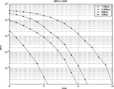
The IEEE 802.11b provides four different physical layer rates 1, 2, 5.5 and 11 Mbps using three different modulation schemes DBPSK, DQPSK and CCK. The bit error probability of DBPSK, DQPSK and CCK in the AWGN channel can be found in several literatures [14]. The performance curves of BER versus SNR for different modulation schemes of the physical layer are shown in Figure 1.

When quality of service parameters such as, BER are given, the most suitable modulation scheme can be chosen by the received SNR.

The 802.11b physical layer has 14 channels, 5 MHz apart in frequency. But to be totally non-overlapping, the frequency spacing must be at least 30 MHz. So the channels 1, 6 and 11 can be used with 802.11b to achieve higher network throughput as multiple transmissions can take place with out interfering with each other. However, the distributed coordinate function (DCF), the basic Medium Access Control (MAC) of IEEE 802.11b, employs carrier sense multiple access with collision avoidance (CSMA/CA) and it is designed for sharing a single channel. As the current 802.11b device is equipped with one half-duplex transceiver, which can switch channels dynamically, can not transmit or receive on one channel at a time. Exploiting multiple channels require dynamic channel negotiation. Such a medium access protocol is MMAC [7] that is capable of dynamic channel negotiation so that multiple communications can take place simultaneously, each in separate channel.

The function of medium access control (MAC) is to enable effective sharing of channel among all nodes in the network. Ideally the MAC should facilitate perfect channel utilization while still being fair to all network flows with in the network. The multi-rate modulation employed in 802.11b leads to fairness problem as shown by [9]. Nodes with low data rate use more channel time than high data rate nodes. As a result not only the low data rate nodes get poor service they also reduce the bandwidth of high data rate nodes. This reduces the effective throughput of the entire network. In this thesis the CD-MMAC (Cooperative Diversity Multi-Channel MAC) protocol attempts to improve the performance of IEEE 802.11b and present detailed analysis of the protocol.

Rest of the thesis is organized as follows: In Chapter 2 an introduction to cooperative transmission is presented. In Chapter 3 we discuss some of the related works on Cooperative MAC protocols. In Chapter 4 we present an overview of the IEEE 802.11b. In Chapter 5 we propose a Multi-Channel MAC protocol incorporating opportunistic cooperative diversity CD-MMAC. In Chapter 6 the simulation environment is presented with radio propagation model, error model and network topologies considered. In Chapter 7 we analyze and evaluate the performance of CD-MMAC with MMAC and IEEE 802.11b with respect to throughput, and delay. Chapter 8 discusses some issues in CD-MMAC and finally Chapter 9 concludes the thesis with a brief summary and possible direction for future work.

CHAPTER 2 INTRODUCTION TO COOPERATIVE TRANSMISSION

The basic ideas behind cooperative communication can be traced back to the groundbreaking work of Cover and El Gamal on the information theoretic properties of the relay channel [2]. This work analyzed the capacity of the three-node network consisting of a source, a destination, and a relay. It was assumed that all three-nodes operate in the same band, so the system can be decomposed into a broadcast channel from the viewpoint of the source and a multiple access channel from the viewpoint of the destination. Many ideas that appeared later in the cooperation literature were first exposited in [2].

However, in many respects the cooperative communication we consider is different from the relay channel. First, recent developments are motivated by the concept of diversity in a fading channel, while Cover and El Gamal mostly analyze capacity in an additive white Gaussian noise (AWGN) channel. Second, in the relay channel, the relay’s sole purpose is to help the main channel, whereas in cooperation the total system resources are fixed, and users act both as information sources as well as relays. Therefore, although the historical importance of [2] is indisputable, recent work in cooperation has taken a somewhat different emphasis.

The wireless channel suffers from fading; the signal attenuation can vary significantly over the course of a given course of a transmission. Transmitting independent copies of the signal generates diversity and can effectively combat the deleterious effects of fading. In particular spatial diversity is generated by transmitting signals from different locations, thus allowing independent faded versions of the signal at the receiver. Cooperative communication generates this diversity in a new way and users can increase their effective quality of service (measured at the physical layer by bit error rate and block error rate) via cooperation.

Figure 2 below illustrates a preliminary example of the ideas of cooperative communications.

S

R

Figure 2: Cooperative Diversity

Two wireless nodes S and D are communicating with each other. Each node has one antenna and cannot individually generate spatial diversity. However it may be possible for node R to receive the signal and forward the signal to the destination. Because the fading paths from two mobiles are statistically independent, this generates diversity.

h

s,r

_h

_r,d

D

CHAPTER 3 RELATED WORKS

Incorporating cooperative diversity at the MAC layer so far has explored two schemes: 1. pre-collision relayed

scheme [2] – When the route is set by the rule of minimum hop nodes chooses high throughput routes based on

received SNR and exchanging extra control packets like HTS (Helper Ready to Send). 2. post-collision buffered

scheme [3] – when there is a collision the collided packets are saved in a buffer. In the slots following the collision a

set of node designed as relays bounce off the signal they received during the collision slot. The receiving node recovers by processing collided packet and the signal forwarded by the relay nodes.

B. Zhao and M. Valenti presented a slotted cross-layer protocol HARBINGER [6] which combines Medium Access Control (MAC) and routing.

CHAPTER 4 OVERVIEW OF IEEE 802.11b

The IEEE 802.11b, the Direct Sequence Spread Spectrum (DSSS) physical layer operates in the 2.4 GHz ISM band. It provides four different physical layer rates 1, 2, 5.5 and 11 Mbps using three different modulation scheme DBPSK (for 1MBps data rate), DQPSK (2MBps data rate) and CCK (for 5.5 and 11 Mbps data rate). The control packets and the header of data packets are always modulated using DBPSK at 1 Mbps. The modulation scheme of data frame is indicated in the physical layer header of the data packet.

The IEEE 802.11b has 14 channels, 5 MHz apart in frequency. But to be totally non-overlapping the frequency must spacing needs to be at least 30 MHz. So typically channel 1, 6 and 11 are used for communication. But the Medium Access Control of IEEE 802.11b is designed for sharing a single channel. The basic Medium Access Control mechanism Distributed Coordinate Function (DCF) and the Power Saving Mechanism (PSM) is of the IEEE 802.11b described below.

IEEE 802.11b DCF

The IEEE 802.11b DCF employs Carrier Sense Multiple Access with Collision Avoidance. By Using the Request To Send (RTS) and Clear To Send (CTS) frames it employs virtual carrier sensing to avoid collision. A source node reserves the channel for data transmission by exchanging RTS/CTS messages with the destination node. When a node wants to send packets to another node, it first sends an RTS (Request to Send) packet to the receiver node. The receiver, on processing the RTS, replies by sending a CTS (Clear to Send) packet to the sender. The RTS and CTS packets include the expected duration of time for which the channel will be in use for data transmission. Other nodes that overhear these packets must defer their transmission for the duration specified in the RTS/CTS packets. For this reason, each node maintains a variable called the Network Allocation Vector (NAV) that records the duration of time it must defer its transmission. This Virtual Carrier Sensing allows the area around the sender and receiver to be reserved for communication. Figure 3 illustrates the operation of IEEE 802.11 DCF.

A B C D A B C D RTS CTS DATA SIFS ACK NAV NAV DIFS Time Contention Window A B C D A B C D RTS CTS CTS DATA DATA SIFS ACK ACK NAV NAV NAV NAV DIFS Time Contention Window Figure 3: IEEE 802.11 DCF

When node B is transmitting a packet to node C, node A overhears the RTS packet and sets its NAV until the end of ACK, and node D overhears the CTS packet and sets it’s NAV until the end of ACK. After the transmission is completed, the stations wait for DIFS and then contend for the channel. In this Figure, node B is a hidden terminal to node D. Without virtual carrier sensing, D would not know of B's transmission. So D may start transmitting a packet to C, while B is transmitting, which results in a collision at C.

If a node has a packet to send but observes the channel to be busy, it performs a random back off by choosing a back off counter no greater than an interval called the contention window. Each host maintains a variable cw, the contention window size, which is reset to a value CWmin when the node is initiated. Also, after each successful transmission, cw is reset to CWmin. After choosing a counter value, the node will wait until the channel becomes idle, and start decrementing the counter. The counter is decremented by one after each “time slot", as long as the channel is idle. If the channel becomes busy, the node will freeze the counter until the channel is free again. When the back off counter reaches zero, the node will try to reserve the channel by sending an RTS to the target node. Since two nodes can pick the same backoff counter, the RTS packet may be lost because of collision. Since the

probability of collision gets higher as the number of nodes increases, a sender will interpret the absence of a CTS as a sign of congestion. In this case, the node will double its contention window to lower the probability of another collision.

Before transmitting a packet, a node has to wait for a small duration of time even if the channel is idle. This is called inter-frame spacing. Four different intervals enable each packet to have different priority when contending for the channel. SIFS, PIFS, DIFS, and EIFS are the four inter-frame spacings, in order of increasing length. A node waits for a DIFS before transmitting an RTS, but waits for a SIFS before sending a CTS or an ACK. Thus, an ACK packet will win the channel when contending with RTS or DATA packets because the SIFS duration is smaller than a DIFS.

IEEE 802.11 PSM

In this section, we describe IEEE 802.11 PSM to explain how ATIM windows are used. A node can save energy by going into doze mode. In doze mode, a node consumes much less energy compared to normal mode, but cannot send or receive packets. It is desirable for a node to enter the doze mode only when there is no need for exchanging data. In IEEE 802.11 PSM, this power management is done based on Ad hoc Traffic Indication Messages (ATIM). Time is divided into beacon intervals, and every node in the network is synchronized by periodic beacon transmissions. So every node will start and finish each beacon interval at about the same time. Figure 4 illustrates the process of IEEE 802.11 PSM. A B C Time Beacon ATIM ATIM-ACK DATA Beacon Figure 4: IEEE 802.11 PSM

At the start of each beacon interval, there exists an interval called the ATIM window, where every node should be in the awake state. If node A has buffered packets for B, it sends an ATIM packet to B during this interval. If B receives this message, it replies back by sending an ATIM-ACK to A. Both A and B will then stay awake for that entire beacon interval. If a node has not sent or received any ATIM packets during the ATIM window (e.g., node C in Figure 2), it enters doze mode until the next beacon time.

ACK ATIM-RES Doze Mode ATIM Window Beacon Interval A B C Time ATIM ATIM-ACK DATA ACK ATIM-RES Doze Mode ATIM Window Beacon Interval

IEEE 802.11 Multi-Rate

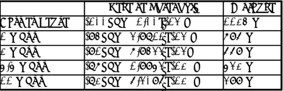
The IEEE 802.11b provides four different physical layer rates 1, 2, 5.5 and 11 Mbps using three different modulation schemes DBPSK, DQPSK and CCK. Figure 3 and Table 1 below, based on the published specifications of a Lucent ORiNOCO PC Card [16], illustrates the approximate transmission range of each data rate:

Carrier Sense Range 1 mbps range 11 mbps range

Figure 5: Transmission Range and Data Rate

399 m -82dbm (6.3096e-12 W) 11 mbps 532 m -87dbm (1.9953e-12 W) 5.5 mbps 669 m -91dbm (7.9433e-13W 2 mbps 796 m -94dbm (3.9811e-13 W) 1 mbps 1124 m -100dbm (1.00e-13 W) Carrier Sense Distance Receive Threshold 399 m -82dbm (6.3096e-12 W) 11 mbps 532 m -87dbm (1.9953e-12 W) 5.5 mbps 669 m -91dbm (7.9433e-13W 2 mbps 796 m -94dbm (3.9811e-13 W) 1 mbps 1124 m -100dbm (1.00e-13 W) Carrier Sense Distance Receive Threshold

CHAPTER 5 CD-MMAC

In this section we present our proposed Multi-Channel Medium Access Control protocol CD-MMAC. It based on the work of Jungmin So of University of Illinois at Urbana Campaign on MMAC [7]. We incorporate opportunistic Cooperative Diversity by exploiting the Control Messages during the ATIM Window of MMAC.

Now we summarize the assumptions before describing the protocol in detail.

Assumptions:

o Each node is equipped with a single transceiver. So that each node can either transmit or listen at a time but can not do both at the same time.

o Transmission power of all nodes is fixed and transmitting nodes choose the best modulation scheme based on the received signal-to-noise ratio (SNR).

o The threshold SNR of each modulation type is predefined and stored in a Physical Mode Table.

o N channels are available for use and all channels have the same bandwidth. Nodes have prior knowledge how many channels are available and the channels are symmetric.

o The transceiver is capable of switching channels and channel switching delay is approximately 224us [15]. o Nodes are synchronized. Each node sends out beacons to synchronize time as in IEEE 802.11 Power Saving

Mechanism (PSM) in a distributed manner.

Protocol Description:

CD-MMAC is an extension of MMAC [7]. Here we divide time into beacon intervals. At the beginning of each beacon interval, all nodes must listen to a predefined common channel for a fixed duration of time (ATIM window). Nodes build and update the Node Rate Info table listening to ATIM messages. Node Rate Info is exchanged by periodic routing updates. In conventional routing nodes selects the minimum hop routes but here nodes select the best routes consulting the Node Rate Info table which is not always minimum hop. Nodes negotiate channels using ATIM messages. Nodes switch to selected channels after ATIM window for the rest of the beacon interval.

Node Rate Info:

Each node maintains a table of all possible relays around itself containing the ID (MAC Address), data rate (based on received SNR) and time (last heard from the relays). During the ATIM Window listening to the ATIM messages nodes will check if the transmitting node is already in the Node Rate Info table. If not a new row is added with the transmitting node’s ID (MAC Address). Then nodes find the data rate between the transmitting node and themselves by checking the Physical Mode Table and update data rate field. The time field will be updated each time a packet from the transmitting node is heard.

Node Rate Info

ID (MAC Address) Value

Data Rate Value

Time Value

Table 2: Data Structure Node Rate Info

This Node Rate Info is exchanged via periodic routing updates. In conventional routing nodes selects the minimum hop routes but here nodes select the best routes consulting the Node Rate Info table which is not always minimum hop.

Preferable Channel List:

Each node maintains a data structure called the Preferable Channel List (PCL), that indicates which channel is preferable to use for the node. PCL records the usage of channels inside the transmission range of the node. Based on this information, the channels are categorized into three states:

• High preference (HIGH): This channel has already been selected by the node for use in the current beacon

interval. If a channel is in this state, this channel must be selected. For each beacon interval, at most one channel can be in this state at each node.

• Medium preference (MID): This channel has not yet been taken for use in the transmission range of the

host. If there is no HIGH state channels, a channel in this state will be preferred.

• Low Preference (LOW): This channel is already taken by at least one the node’s immediate neighbors. To

balance the channel load as much as possible, there is a counter for each channel in the PCL to record how many source-destination pairs plan to use the channel for the current interval. If all channels are in LOW state, a node selects the channel with the smallest count.

The channel states are changed in the following way:

• All the channels in the PCL are reset to MID state when the node is powered up, and at the start of each

beacon interval.

• If the source and destination nodes agree upon a channel, they both record the channel to be in HIGH

• If a node overhears an ATIM-ACK or ATIM-RES packet (explained in the next section), it changes the

state of the channel specified in the packet to be LOW, if it was previously in the MID state. When the state of a channel changes from MID to LOW, the associated counter is set to one. If the channel was previously in HIGH state, it stays in the HIGH state. If the channel was already in the LOW state, the counter for the channel is incremented by one.

Channel Negotiation:

As in MMAC, in CD-MMAC periodically transmitted beacons divide time into beacon intervals. A small window called the ATIM window is placed at the start of each beacon interval (we use the term “ATIM” as in IEEE 802.11 PSM, although it is used for a different purpose in our protocol). The nodes that have packets to transmit negotiate channels with the destination nodes during this window. In the ATIM window, every node must listen to the default

channel. The default channel is one of the multiple channels, which is predefined so that every node knows which

channel is the default channel. During the ATIM window, all nodes listen on the default channel, and beacons and ATIM packets are transmitted on this channel. Outside the ATIM window, the default channel is used for sending data, similar to other channels.

A

B

C

D

N o d e R a te In fo

Figure 6: Channel Negotiation and Node Rate Info exchange in CD-MMAC

If node S has buffered packets destined for D, it will notify D by sending an ATIM packet. S includes its preferable channel list (PCL) in the ATIM packet. D, upon receiving the ATIM packet, selects one channel based on the

sender’s PCL and its own PCL. As explained in the next section, the receiver’s PCL has higher priority in selecting the channel. After D selects a channel, it includes the channel information in the ATIM-ACK packet and sends it to S. When S receives the ATIM-ACK packet, it sees if it can also select the channel specified in the ATIM-ACK. S can select the specified channel only except when S has already selected another channel. If S selects the channel specified in the ATIM-ACK, S sends an ATIMRES packet to the D, with S’s selected channel specified in the packet. The ATIM-RES packet notifies the nodes in the vicinity of S which channel S is going to use, so that the neighboring nodes can use this information to update their PCL. Similarly, the ATIM-ACK packet notifies the nodes in the vicinity of D. After the ATIM window, S and D will switch to the selected channel and start communicating by exchanging RTS/CTS. If S cannot select the same channel as D, because it has already selected another channel, it cannot send packets to D during the beacon interval. It has to wait for the next beacon interval to negotiate channels again.

When multiple nodes start sending ATIM packets at the beginning of a beacon interval, ATIM packets will collide with each other. To avoid such collisions, each node waits for a random backoff interval before transmitting an ATIM packet. The backoff interval is chosen in the range [0, CWmin].

Rules for selecting the Channel:

When a node receives an ATIM packet, it selects a channel and notifies the sender by including the channel information in the ATIM-ACK packet. The receiver tries to select the “best” channel based on information included in the sender’s PCL (preferable channel list) and its own PCL. The best channel is the channel with the least scheduled traffic, as elaborated below. This selection algorithm attempts to balance the channel load as much as possible, so that bandwidth waste caused by contention and backoff is reduced. For this reason, the number of source-destination pairs that have selected the channel is counted by overhearing ATIM-ACK and ATIM-RES packets and select the one with the lowest count. This scheme assumes that every source-destination pair will deliver the same amount of traffic in a beacon interval, which may not be true.

Suppose that node A has packets for B and thus sends an ATIM packet to B during the ATIM window, with A’s PCL included in the packet. On receiving the ATIM request from A, B decides which channel to use during the beacon interval, based on its PCL and A’s PCL. The selection procedure used by B is described as follows.

1. If there is a HIGH state channel in B’s PCL, this channel is selected. 2. Else if there is a HIGH state channel in A’s PCL, this channel is selected.

3. Else if there is a channel which is in the MID state at both A and B, it is selected. If there are multiple channels in this state, one is selected arbitrarily.

4. Else if there is a channel which is in the MID state at only one side, A or B, it is selected. If there are multiple of them, one is selected arbitrarily.

5. If all of the channels are in the LOW state, add the counters of the sender’s PCL and the receiver’s PCL. The channel with the least count is selected. Ties are broken arbitrarily.

After selecting the channel, B sends an ATIM-ACK packet to A, specifying the channel it has chosen. When A receives the ATIM-ACK packet, A will see if it can also select the channel specified in the ATIM-ACK packet. If it can, it will send an ATIM-RES packet to B, with A’s selected channel specified in the packet. If A cannot select the channel which B has chosen, it does not send an ATIM-RES packet to B.

CHAPTER 6 SIMULATION ENVIRONMENT

The Network Simulator NS-2 [10], version 2.1b9a, has been used to simulate the proposed CD-MMAC protocol and to perform comparisons with MMAC and 802.11b. NS-2 is a widely used open source simulator that offers built-in 802.11 MAC layer and the implementation of the most common routing protocols. In order to correctly simulate the proposed CD-MMAC protocol several improvements in NS-2 was implemented.

Although widely used, NS-2 presents some limitations, mostly in the modeling of the physical layer and MAC layer. At the physical level, an extension of NS-2, which allows the simulation of Ricean and Rayleigh fading was implemented. In NS-2 the radio interface model is still based on old WaveLAN cards, thus lacking in correct support of rates higher than 2 Mbps. To support multi-rate transmissions both physical layer and MAC layer was implemented as defined in standard 802.11b [15]. The interface parameters were set to model the Lucent ORiNOCO PC Card [16] features, which are summarized in TABLE 1. The last piece that was added to NS-2 is a cross-layer MAC enabling route selection by the rule of minimum delay thus incorporating cooperative diversity as described in Chapter 5.

The simulations were performed in a sixteen node wireless LAN scenario where each node is placed at distance of 300 meters horizontally and vertically. Each source node generates and transmits constant-bit-rate (CBR) traffic of 512 bytes. The transmission power is fixed at 15 dbm. For CD-MMAC and MMAC number of channel used is 3, the beacon interval is set to 100 ms and ATIM window is set 20 ms. Each simulation was performed for duration of 40 seconds.

CHANNEL MODEL AND ERROR MODEL

The error model used in the simulation was based on the detailed simulation of a Rayleigh fading channel as described in [11] to model packet errors. The implementation of Ricean Fading Model is based on CMU additions to

NS to handle Ricean and Rayleigh fading [10]. Although, the CMU implementation results in an accurate simulation

of the wireless channel for each individual flow, the fading components of channels for different flows are identical, a scenario not encountered in practice. This arises due to the fact that the index into the pre-computed channel table (used to look-up the components of fading envelope) is chosen based on the simulator's time instant, which is identical for all flows. To more realistically model the wireless channel for multiple users the implementation was modified such that channel lookup indexes are a function of the flow and time according to [12].

In reality, the channel quality of wireless nodes can vary significantly, both for mobile and stationary nodes. In particular, a node's received signal is composed of both a line-of-sight component as well as numerous delayed signals reflected off of surrounding objects. All such signals (plus random noise) combine and must be decoded by the receiver. In favorable cases, these signals add coherently in a way that enhances the channel quality (increases received power, increases signal-to-noise ratio, etc.). However, in unfavorable cases, these signals will tend to cancel each other out and lead to a poor-quality channel. Even for stationary nodes, any change in the line-of-sight path or any reflected path (e.g., due to an intermediary pedestrian) will change the quality of the channel and hence, change the received signal power.

The transmitted radio frequency signal is reflected by both natural and man-made objects. Thus, the signal at the receiver is a superposition of different reflections of the same signal, received with varying delays and attenuations. Based on the relative phases of different reflections at the receiver, the different copies of the same signal may add coherently or tend to cancel out. Coherent addition of the copies can result in large received signal powers and cancellation eventually leads to zero received signal power. The signal power strength is heavily dependent on the spatial location of the transmitter, receiver, the reflecting objects and the material of the reflecting objects.

Physical layer design and analysis typically consider detailed propagation models that characterize all reflections and their time-variations [14]. An accurate and widely utilized model which considers time-varying multi-path propagation [16] is ( ) 1

( )

( ) (

( ))

( )

p t i i i

y t

A t x t

t

z t

=

=

∑

− τ

+

where

x t

( )

is the transmitted signal and is the received signal. The time-varying multi-path propagation is captured by the attenuation of each path

( )

y t

( )

i

A t

, the time delays

τ

i

( )

t

and the number of paths . The additive

term is generally labeled as the background noise and represents the thermal noise of the receiver. The loss

( )

p t

( )

suffered by the signal during its propagation along different paths is captured in

A t

i

( )

, and depends on the distance

between the sender and the receiver.

Typically, physical layer algorithms (error correcting codes, channel modulation, demodulation and decoding) use the elaborate models in Equation (1). The performance of any physical layer implementation is well captured by observing its packet loss rate as a function of the received signal to noise ratio (SNR). Received signal to noise ratio measures the extent of the received signal power over the channel background noise. Typically, the larger the SNR, the better the chance of any packet being received error free. Actual performance (packet loss rate as a function of SNR) is dependent on a particular implementation.

Recognizing that the received SNR can be used to capture the packet level performance of any physical layer implementation, the following model was used for the received signal to noise ratio for transmitter power at packet transmission time

P

p

t

2

( )

( )

p

( )

p p

t

SNR t

=

Pd t

−β

ρ

σ

where

d t

( )

p is the distance between the sender and the receiver at time

t

p,

β

is the path loss exponent,

ρ

( )

t

p is

the average channel gain for the packet at time

t

p, and

σ

2 is the variance of the background noise

z t

( )

.

The short time-scale variation in the received SNR is captured by the time-varying parameter , known as the fast fading component of the fading process. The time-variation of

( )

t

p

ρ

( )

t

p

ρ

is typically modeled by a probability distribution and its rate of change. An accurate and commonly used distribution for

ρ

( )

t

p is the Ricean distribution,

2 ( ) 2 ₀ 2

( )

(2

)

K

p

e

I

ρ − + σ

ρ

K

ρ =

ρ

σ

where

K

is the distribution parameter representing the strength of the line of the sight component of the received signal and

I

0

(2

K

ρ

)

is the modified Bessel function of the first kind and zero-order. For , the Ricean

distribution reduces to the Rayleigh distribution, in which there is no line-of-sight component.

0

K

=

The rate of change of depends on a mobile node's relative speed with respect to its surroundings. Among the several models available in the literature we use the Clarke and Gans model [16]. The motion of nodes causes a Doppler shift in the frequency of the received signal, and the extent of the Doppler shift depends on the relative velocity of the sender and the receiver. Let

( )

t

p

ρ

m

f

denote the maximum Doppler frequency during the communication between the two nodes. Then according to the

2

1.5

( )

1

c m m

S f

f

f

f b

f

=

⎛

−

⎞

π

_{− ⎜}

_⎟

⎝

⎠

Here,

f

c represents the carrier frequency of the transmitted signal. The spectral shape of the Doppler spectrum in

this determines the time domain fading waveform and hence the temporal correlation. The inverse of the maximum Doppler frequency of

f

m,

1

c m

T

f

=

known as the coherence interval, and represents the average time of

decorrelation. In essence, the channel SNR values

ρ

( )

t

p separated by more than

t

c, are approximately independent.

For the purpose of simulation a dataset containing the components of a time-sequenced fading envelope is pre-computed. It is assumed that the small scale fading envelope is used to modulate the calculations of a large scale propagation model (two-ray ground model).

Computation of the dataset is performed as described in the literature [8], [7]. In-phase and quadrature phase components are generated using a Gaussian distribution, then spectrally shaped by the Doppler spectrum. The model of Clarke and Gans is used for the Doppler power spectral density [3], [5]. The dataset essentially contains a sequence of in-phase and quadrature components which are then combined (with the appropriate Ricean K factor) within the simulator to yield the fading envelope. With K=0 the dataset yields Rayleigh fading envelope.

The following steps are taken to create the dataset:

1. Specify the number of points, the maximum Doppler frequency,

f

m, and the frequency spacing of the points

used. The frequency spacing determines the time duration.

2. Generate complex Gaussian random numbers for each of the frequency components. The complex frequency component at any particular frequency and at its negative frequency should be complex conjugates. This will yield a real waveform.

3. Create the fading spectrum, evaluated at the same frequency points as above.

4. Multiply the frequency domain components with the fading spectrum.

5. Perform an IFFT on this data to yield a time series data.

These two sets form the in-phase and quadrature phase multipath sources.

The process of performing the IFFT on this low-pass filtered frequency domain data ensures that the beginning and end of the dataset if wrapped around do not have discontinuities.

For the purposes of simulation, it is convenient to store the in-phase and quadrature-phase multipath sources

x

1, 2

x

, normalized to have unity variance.

A Ricean amplitude with parameter

K

can be created by combining the quadrature components

x

1,

x

2, from the

dataset as

2 2

1

)

2

r

= (σ +

x

A

+ σ

x

where

A

2

/(2

σ ≡

2

)

K

and

σ

x

i is a random variable with variance

σ

2

The mean-squared value of the Ricean distribution is given by

2 2 2

2

2

(

A

+ σ = σ

K 1)

+

The normalized power envelope is therefore

2 2 2 1 2

1

(

2

)

2(

1)

r

x

K

x

P

K

⎡

⎤

=

_⎣

+

+

_⎦

+

This power envelope is used to modulate the output of a large scale propagation model. It is assumed that the mean squared value of the envelope is the power predicted by the large scale model.

NETWORK TOPOLOGY

The following topologies were considered to evaluate the performance of the wireless network. Firstly in the chain topology 802.11b DCF is evaluated against the proposed cooperative transmission in 802.11b DCF termed as CD-DCF. Finally in the grid topology the performance of CD-MMAC is evaluated with respect to MMAC and 802.11b DCF.

Chain topology:

In this topology 4 nodes are placed in a strait line with 300 meters apart as shown in the figure below.

11 m bps link 1 m bps link 11 m bps link 0 1 2 3 11 m bps link 1 m bps link 11 m bps link 0 1 2 3

Figure 7: Chain Topology

Here node 0 is the source of communication and node 2 is the destination which is approximately 600 meters away. There is only one flow in this topology.

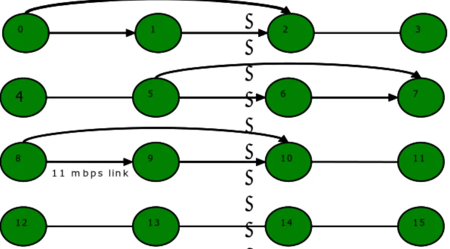
Grid topology:

A 4 by 4 grid is used in this topology. The distance between nodes is approximately 300 meters both in vertical and horizontal direction. Here nodes 0, 5 and 8 are the source of communication while nodes 2, 7 and 10 are the destination of the communication. There are three flows in this topology. All the three flows start and stop at the same time. 1 m b p s lin k 1 1 m b p s lin k 0 1 2 3 4 5 6 7 8 9 1 0 1 1 1 2 1 3 1 4 1 5 1 m b p s lin k 1 1 m b p s lin k 0 1 2 3 4 5 6 7 8 9 1 0 1 1 1 2 1 3 1 4 1 5

CHAPTER 7 SIMULATION RESULTS

In this section the simulation results are presented. In the graphs the curves labeled as “802.11b DCF” refer to original IEEE 802.11b single channel MAC, the curves labeled as “802.11b CD-DCF” refer to cooperative 802.11b single channel MAC, the curves labeled as “MMAC” refers to Multi-Channel MAC and the curves labeled as “CD-MMAC” refers to the proposed cooperative Multi-Channel MAC.

Chain Topology:

Firstly we present the results from simulation performed on the Chain Topology with only a single flow as shown in the figure. Figure 9 shows the aggregate throughput of different protocols as the network load increases.

Figure 9: Load vs Throughput Chain Topology

Figure 10: Delay vs Load Chain Topology

As the network load increases the cooperative DCF significantly better than the IEEE 802.11b. Figure 10 shows the average packet delay of the protocols as the network load increases. WE can see that the cooperative DCF clearly outperforms the IEEE 802.11b DCF.

Grid Topology:

We now present the results from simulation performed on the Grid Topology as shown in the figure. Figure 11 shows the aggregate throughput of different protocols as the network load increases. When the network load is minimal all the protocols performs similarly. As the network load increases MMAC performs better than IEEE 802.11b DCF and the CD-MMAC performs much better than MMAC.

Figure 11: Throughput vs Load Grid Topology

Figure 12 shows the average packet delay of all the protocols. Here MMAC shows the least average packet delay. But CD-MMAC shows smaller packet delay compared to the IEEE 802.11b DCF.

The reason CD-MMAC shows higher packet delay than MMAC is because packets have to wait during the channel negotiation phase (ATIM Window) more than MMAC as the packets are going through a relay, although CD-MMAC achieves higher throughput than CD-MMAC. So we can clearly see that CD-CD-MMAC clearly outperforms IEEE 802.11b DCF in terms of throughput and delay.

CHAPTER 8 ISSUES IN CD-MMAC

As in CD-MMAC we are always using the high throughput nodes as relays there is a possibility that the relay nodes become congested. Figure 13 below illustrates the situation:

N o d e R C o n g e s t e d S S S R D D D

CHAPTER 9 CONCLUSION AND FUTURE WORK

In this paper we proposed a new MAC protocol CD-MMAC for 802.11b Wireless Networks. The protocol utilizes multiple channels dynamically using a single interface and incorporates opportunistic cooperative diversity and makes better use of the multiple transmission rates offered by the PHY layer. The performance improvement in CD-MMAC is evaluated by extensive simulation and analysis. The simulation result shows the protocol improves network throughput and packet delivery ratio significantly and reduces packet delay. In future we would like to work on the previously described congestion problem at the relay nodes.

REFERENCES

[1] A. Nosratinia, T.E. Hunter, A. Hedayat, "Cooperative communication in wireless networks", Communications Magazine, IEEE On, vol. 42, issue: 10, pp. 74- 80, Oct. 2004

[2] T. M. Cover and A. A. E. Gamal, “Capacity Theorems for the Relay Channel,” IEEE Trans. Info. The ory, vol. 25, no. 5, Sept. 1979, pp. 572–84.

[3] A. Sendonaris, E. Erkip, and B. Aazhang, “User Cooperation Diversity Part I and Part II,” IEEE Trans.

Commun., vol. 51, no. 11, Nov. 2003, pp. 1927–48.

[4] Pei Liu, Zhifeng Tao and Shivendra Panwar, “A Cooperative MAC Protocol for Wireless Local Area Networks”, IEEE Trans. Commun., vol. 5,

[5] Rui Lin and Athina P. Petropulu, “Cooperative transmission for random access wireless networks”,

[6] B. Zhao and M. Valenti, “Practical relay networks: a generalization of hybrid-ARQ,” IEEE Journal on Selected

Areas in Communications, vol. 23, no. 1, Jan. 2005.

[7] Jungmin So and Nitin Vaidya, “MultiChannel MAC for Ad Hoc Networks: Handling MultiChannel Hidden Terminals Using A Single Transceiver”, In ACM MobiHoc 2004.

[8] Wireless LAN Medium Access Control (MAC) and Physical Layer (PHY) specifications, IEEE Std. 802.11b, 1999.

[9] M. Heusse, F. Rousseau, G. Berger-Sabbatel, and A. Duda, “Performance anomaly of 802.11b,” in Proc. of

IEEE INFOCOM, San Francisco, USA, March-April 2003.

[10] The Network Simulator NS-2 available: http://www.isi.edu/nsnam/ns/

[11] Ratish J. Punnoose, Pavel V. Nikitin, and Daniel D. Stancil. Efficient Simulation of Ricean Fading within a

Packet Simulator Vehicular Technology Conference, Sept 2000.

[12] B. Sadeghi, V. Kanodia, A. Sabharwal, and E. Knighlty, “Opportunistic Media Access for Multirate Ad Hoc Networks'', in Proceedings of ACM MobiCom'02 , Atlanta, Giorgia, September 2002.

[14] J. G. Proakis, Digital Communications (Fourth edition). McGraw Hill, 2001.

[15] IEEE 802.11 Working Group, “Wireless LAN Medium Access Control (MAC) and Physical Layer (PHY) specifications,” 1997.