Automatic Detection of Low Passability Terrain Features in the Scandinavian Mountains

(1)

IN THE FIELD OF TECHNOLOGY DEGREE PROJECT

CIVIL ENGINEERING AND URBAN MANAGEMENT AND THE MAIN FIELD OF STUDY

INFORMATION AND COMMUNICATION TECHNOLOGY, SECOND CYCLE, 30 CREDITS

,

STOCKHOLM SWEDEN 2019

Automatic Detection of Low

Passability Terrain Features in the

Scandinavian Mountains

(2)

Author: Fredrik Ahnlén

Title: Automatic Detection of Low Passability Terrain Features in the Scandinavian Mountains Supervisor: Milan Horemuz

Examiner: Huaan Fan

TRITA: TRITA-ABE-MBT-19435

Keywords: Classification, Fuzzy Logic, Fuzzy Inference System, Automatic Mapping, Terrain Features, Land Cover Mapping, Cartography, Shrub, Mire, Stony Ground

(3)

Acknowledgments

Milan Horemuz, KTH Geodesy and Geoinformatics, co-supervisor. For assisting in the structur-ing of the thesis as well as providstructur-ing helpful feedback and technical support.

Huaan Fan, KTH Geodesy and Geoinformatics, examiner.

Oskar Karlin, Calazo Förlag AB, co-supervisor. For providing good technical support and knowledge of the study area.

Finally big thanks to Fredrik Hjelmstedt, Calazo Förlag AB, for providing the possibility to write the thesis in collaboration with Calazo, Henrik Johansson, Calazo Förlag AB, for provid-ing technical support, Andreas Rönnberg, Lantmäteriet Geodata, for providprovid-ing technical LiDAR support, Birgitta Olsson, Naturvårdsverket, Luke Webber, Metria and Camilla Jönsson, Metria for providing support regarding Neural Networks and remote sensing classification of mires and Joakim Svensk, Foran Sverige AB for providing initial tips for the thesis approach.

(4)

Abstract

During recent years, much focus have been put on replacing time consuming manual mapping and classification tasks with automatic methods, having minimal human interaction. Now it is possible to quickly classify land cover and terrain features covering large areas to a digital format and with a high accuracy. This can be achieved using nothing but remote sensing techniques, which provide a far more sustainable process and product. Still, some terrain features do not have an established methodology for high quality automatic mapping.

The Scandinavian Mountains contain several terrain features with low passability, such as mires, shrub and stony ground. It would be of interest to anyone passing the land to avoid these areas. However, they are not sufficiently mapped in current map products.

The aim of this thesis was to find a methodology to classify and map these terrain features in the Scandinavian Mountains with high accuracy and minimal human interaction, using remote sensing techniques. The study area chosen for the analysis is a large valley and mountain side south-east of the small town Abisko in northern Sweden, which contain clearly visible samples of the targeted terrain features. The methodology was based on training a Fuzzy Logic classifier using labeled training samples and descriptors derived from ortophotos, LiDAR data and current map products, chosen to separate the classes from each other by their characteristics. Firstly, a set of candidate descriptors were chosen, from which the final descriptors were obtained by implementing a Fisher score filter. Secondly a Fuzzy Inference System was constructed using labeled training data from the descriptors, created by the user. Finally the entire study area was classified pixel-by-pixel by using the trained classifier and a majority filter was used to cluster the outputs. The result was validated by visual inspection, comparison to the current map products and by constructing Confusion Matrices, both for the training data and validation samples as well as for the clustered- and non-clustered results.

The results showed that the low passability terrain features mire, shrub and stony ground, can indeed be mapped with high accuracy using this methodology and that the results are generally clearly better then the current map products. However, to be optimised, the methodology could be further fine-tuned by implementing soil wetness descriptors and higher spatial resolution LiDAR as well as using a more widespread choice of classes.

Keywords: Classification, Fuzzy Logic, Fuzzy Inference System, Automatic Mapping, Terrain Features, Land Cover Mapping, Cartography, Shrub, Mire, Stony Ground

(5)

Sammanfattning

De senaste åren har mycket fokus lagts på att ersätta tidskrävande manuella karterings- och klas-sificeringsmetoder med automatiserade lösningar med minimal mänsklig inverkan. Det är numera möjligt att digitalt klassificera marktäcket och terrängföremål över stora områden, snabbt och med hög noggrannhet. Detta med hjälp av enbart fjärranalys, vilket medför en betydligt mer hållbar process och slutprodukt. Trots det finns det fortfarande terrängföremål som inte har en etablerad metod för noggrann automatisk kartering.

Den skandinaviska fjällkedjan består till stor del av svårpasserade terrängföremål som sank-marker, videsnår och stenig mark. Alla som tar sig fram i terrängen obanat skulle ha nytta av att kunna undvika dessa områden men de är i nuläget inte karterade med önskvärd noggrannhet.

Målet med denna analys var att utforma en metod för att klassificera och kartera dessa ter-rängföremål i Skanderna, med hög noggrannhet och minimal mänsklig inverkan med hjälp av fjärranalys. Valet av testområde för analysen är en större dal och bergssida sydost om Abisko i norra Sverige som innehåller tydliga exemplar av alla berörda terrängföremål. Metoden baser-ades på att träna en Fuzzy Logic classifier med manuellt utvald träningsdata och deskriptorer, valda för att bäst separera klasserna utifrån deras karaktärsdrag. Inledningsvis valdes en uppsät-tning av kandidatdeskriptorer som sedan filtrerades till den slutgiltiga uppsätuppsät-tningen med hjälp av ett Fisher score filter. Ett Fuzzy Inference System byggdes och tränades med träningsdata från deskriptorerna vilket slutligen användes för att klassificera hela testområdet pixelvis. Det klassifi-cerade resultatet klustrades därefter med hjälp av ett majoritetsfilter. Resultatet validerades genom visuell inspektion, jämförelse med befintliga kartprodukter och genom confusion matriser, vilka beräknades både för träningsdata och valideringsdata samt för det klustrade och icke-klustrade resultatet.

Resultatet visade att de svårpasserade terrängföremålen sankmark, videsnår och stenig mark kan karteras med hög noggrannhet med hjälp denna metod och att resultaten generellt är tydligt bättre än nuvarande kartprodukter. Däremot kan metoden finjusteras på flera plan för att opti-meras. Bland annat genom att implementera deskriptorer för markvattenrörelser och användande av LiDAR med högre spatial upplösning, samt med ett mer fulltäckande och spritt val av klasser.

(6)

3.1.1 Detection of wetlands . . . 19 3.1.2 Detection of vegetation . . . 19 3.1.3 Detection of rocks . . . 20 3.2 Neural Networks . . . 20 3.3 Fuzzy Logic . . . 20 3.4 Descriptors . . . 22 4 Research Methodology 24 4.1 Approach . . . 24 4.2 Software description . . . 25 4.3 Data collection . . . 25 4.4 Analysis . . . 27

4.4.1 Candidate descriptor selection . . . 27

4.4.2 Data pre processing . . . 32

4.4.3 Training samples and calculation of descriptors . . . 33

4.4.4 Building FIS . . . 34 4.4.5 Classification . . . 35 4.4.6 Validation . . . 36 5 Results 37 5.1 Classification results . . . 37 5.2 Comparison to Lantmäteriet . . . 45 5.3 Confusion Matrices . . . 46

(7)

6 Discussion 49

7 Conclusions 53

8 Future Work 53

(8)

List of Figures

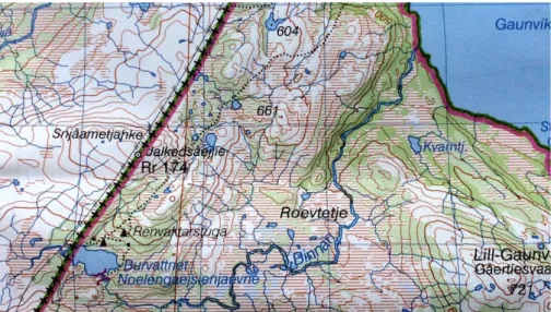
1 The GSD-Mountain Map at the Swedish-Norwegian border. . . 2

2 The GSD-Topographic Map. . . 3

3 The GSD-Property Map. . . 3

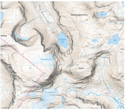
4 A high alpine Calazo map in Abisko, northern Sweden. . . 4

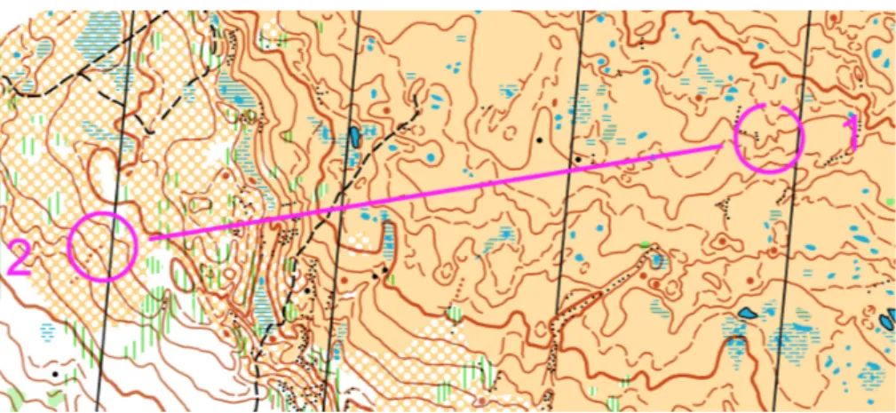
5 A very detailed orienteering map in alpine terrain. . . 5

6 The study area. . . 6

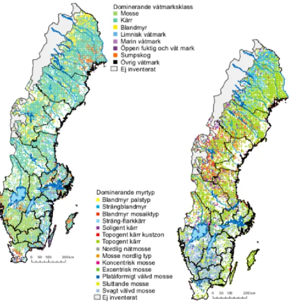
7 Dominating wetland type (left) and mire type (right). . . 10

8 A typical bog with thick turf layer. . . 11

9 A fen with a characteristic pattern. . . 11

10 Stony ground in the alpine zone. . . 12

11 Dwarf Birch (Betula nana). . . 13

12 Grey Willow (Salix glauca). . . 13

13 Downy Willow (Salix lapponum). . . 14

14 Wooly Willow (Salix lanata). . . 14

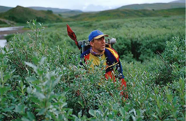
15 A typical very dense willow shrub in the alpine zone. . . 14

16 Satellite imagery. . . 16

17 Aerial imagery. . . 17

18 Overlapping images. . . 17

19 LiDAR scanning. . . 18

20 Methodology float chart. . . 24

21 Spectral reflectance characteristics of water, dry soil and vegetation in the visible and infrared spectrum [1]. . . 27

22 Roughness, based on height above ground. . . 28

23 Roughness, based on normal differences. . . 29

24 Roughness, based on distance to best fitting plane. . . 30

25 Study Area Ortophoto RGB. . . 37

26 Classified result, non-clustered. . . 38

27 Classified result, clustered. . . 39

28 Ortophoto RGB, mire and shrub region. . . 40

31 Ortophoto RGB, shrub and stony region. . . 42

34 Ortophoto RGB, misclassified shrub region. . . 44

(9)

List of Tables

1 Data description . . . 26

2 Chosen candidate descriptors . . . 32

3 FIS settings . . . 34

4 Final descriptors . . . 35

5 Confusion Matrix - Non-clustered - Training Area . . . 47

6 Confusion Matrix - Clustered - Training Area . . . 47

7 Confusion Matrix - Non-clustered - Validation Area . . . 48

(10)

Terms and Abbrevations

Descriptors: In many researches and reports, the classification descriptors that are used to sepa-rate classes are called features. Since the term feature could be misinterpreted as a physical object and be mixed up with the term terrain feature, the term descriptor is used instead.

Low Passability Terrain Features: By low passability terrain feature is meant terrain features that are significantly harder or slower to pass than a similar area that is not affected by the terrain feature. Thus, the general character of the terrain decides what is normal or high passability. That means that, for the Scandinavian Mountains, all land cover without e.g. dense vegetation, shrubs, stony ground, wetlands etc. will be considered as having normal passability while e.g. very steep slopes or cliffs, water bodies, shrubs, mires, stony ground etc. are low passability terrain features. CNN: Convolutional Neural Networks

DEM: Digital Elevation Model DTM: Digital Terrain Model DTW: Depth To Water

FCN: Fully Connected Network FIS: Fuzzy Inference System

GNSS: Global Navigation Satellite Systems HAG: Height Above Ground

ILSVRC: ImageNet Large-Scale Visual Recognition Challenge ISOM: International Specification for Orienteering Maps LiDAR: Light Detection And Ranging

LM: Lantmäteriet, The Swedish mapping, cadastral and land registration authority MF: Membership Function

MFI: Markfuktighetsindex, Ground Moist Index

NMD: Nationella Marktäckedata, National land cover data NDVI: Normalised Differential Vegetation Index

NVV: Naturvårdsverket, Swedish Environmental Protection Agency SAR: Synthetic Aperture Radar

SR: Simple Ratio Vegetation Index SVM: Support Vector Machine UNB: University of New Brunswick

(11)

1 Introduction

During the recent decades, the ongoing worldwide digitisation process has dramatically changed our way of collecting, handling and storing data. A digital representation of data is both easier and less time consuming to maintain, process and analyse, compared to analogue representa-tions. The digitisation is providing solutions for a sustainable development of many sectors of the society, including GIS and cartographic applications. To fully understand the geographical extent of our earth, we have been producing maps for thousands of years. Visualising 3D topo-graphic information on a projected 2D surface make simple interpretation and navigation possible. However, traditional mapping techniques based on extensive field work is very time consuming. The increasing availability of high resolution data covering large areas has made accurate land cover classification with minimal human interaction possible, mostly thanks to remote sensing techniques. Digital methods are developed to automatically extract terrain features from remote sensing imagery and has revolutionised the world of cartography, providing new sustainable solu-tions. Now it is possible to accurately represent terrain features on maps of unknown areas, with minimal manual interaction or field works. Various classification and machine learning tech-niques have already been developed for e.g. image and point cloud classification. However, there are still terrain features that lack an established methodology for detection and extraction. In the Scandinavian Mountains, maps of today do not adequately represent some low passability terrain features such as mires, stony ground or shrubs. Mapping these would clearly improve the use-fulness of terrain maps for hikers, campers or anyone passing the landscape off-trail. This thesis investigates ways of automatic mapping of the terrain features mires, stony ground and shrubs in the Scandinavian Mountains with the aim to find a methodology for accurate and automatic mapping.

1.1 Objectives

The low passability terrain features mires, stony ground and shrubs are not adequately mapped in current maps of the Scandinavian Mountains. The objective of this research is to develop a methodology that adequately classify and map mires, stony ground and shrubs in the Scandinavian Mountains automatically, using aerial images and LiDAR data. Furthermore, the objective is to implement and validate this methodology for a particular study area.

1.2 Current maps and usage

The mapping of the Swedish landscape was initialised in the early 16th century and was thus very late compared to the international mapping progress [2]. One of the pioneers was Andreas

(12)

surveying is performed for the mapping purpose. Instead, the data collection and updates are performed by using remote sensing techniques.

The LM map information has been used to create specific map products, containing informa-tion adapted for certain purposes. The maps covering the Scandinavian Mountains have mainly originated from the 1:50 000 map series known as the GSD-Mountain Map [4], which includes basic information such as e.g. roads, buildings, lakes and names but also contours, mires, streams, open/vegetated areas, trails, important bridges etc, see Figure 1. Since 2018, due to decreasing demands, those maps are no longer provided and users are instead referred to various online map services. The specific mountain information, such as trails, paths etc., is however available in the product GSD-Mountain Information. Two other map products are the GSD-Topographic Map and the GSD-Property Map. The topographic map is a 1:50 000 map with complete land cover rep-resentation, including e.g. rocky ground with blocks and coniferous/deciduous forest, see Figure 2. The GSD-Property Map is the most detailed map provided by LM, containing property infor-mation but also topographic inforinfor-mation, produced for the scale interval 1:5 000 to 1:20 000, see Figure 3 [3].

(13)

(14)

an even higher resolution and level of detail. Today, some of the most used maps are provided by Calazo Förlag AB, which produce maps in 1:100 000 and 1:50 000 scale covering the Scandina-vian Mountains but also high alpine maps of scales 1:15 000 to 1:25 000, see Figure 4. The Calazo maps use much of the available information from LM together with various other data sources. The data acquisition from LM has significantly improved lately, now using more digital land clas-sification techniques and currently (2017-2019), the Swedish Environmental Protection Agency (NVV), is performing a detailed national land cover classification named Nationella Marktäcke-data (NMD). It is a new 10 m resolution Marktäcke-database with the purpose of mapping fundamental information of the landscape and its changes [5]. The database is constructed with the aid of e.g. satellite images, groundwater movement and LiDAR data and it includes various vegetation types located on or off wetlands. Thus NMD provides the most updated and accurate mapping of mires, but so far the algorithm is not adequately handling wetlands on slopes and the Scandina-vian Mountains are not yet classified. To deal with the misclassification on slopes, a method using a Convolutional Neural Network (CNN), trained on 10 m resolution Sentinel-2 satellite images is used for the mapping of the mountain region. The results are going to be published in 2019 and could probably be used to adequately represent the general existence of mires. But small details or small areas would be missed by the 10 m resolution classification. The NMD also does not include shrub or stony ground.

Figure 4: A high alpine Calazo map in Abisko, northern Sweden.

The most detailed terrain maps available today are those produced according to the International Specification for Orienteering Maps (ISOM) to be used in the sport of Orienteering [6]. The maps are produced by extensive field work by a cartographer, using base material from e.g. LiDAR data,

(15)

aerial images and georeferenced topographic data from LM, such as roads, buildings, streams, etc. The maps represent all visible features relevant for an orienteer to navigate at running speed, such as vegetation density, features with varying ground runability and other features such as rocks, streams and even distinct individual trees. See Figure 5 where the vertical green stripes represent shrub, small black dots represent stony ground and horizontal blue stripes represent mires.

Figure 5: A very detailed orienteering map in alpine terrain.

In general, the maps are and have always been used by people traveling the landscape, either along existing trails or off-trail. The generally smooth landscape makes it possible to hike, run or ski in most areas without any advanced safety equipment. Due to the lack of mobile signals in these remote areas, digital maps are difficult to use and a printed map and compass is usually the only navigational tools used, preferably complimented by a GNSS device.

(16)

1.3 Study area

The study area chosen for the analysis is located in northern Sweden south-east of the village Abisko, see Figure 6. This area fulfills several of the requirements and characteristics previously described in this section.

• It covers a pre alpine to alpine zone in the Scandinavian Mountains.

• It contains clearly visible samples of all desired low passability features; mires, stony ground and shrub.

• It contains both steep high alpine peeks and smooth flat valleys.

• Relevant data sources from relevant time periods are available for the entire area.

(17)

Even if the shrub, such as willows can be found in the entire mountain range, they are much more distinct in the northern regions where they can sometimes cover entire alpine valleys and thus cause a much bigger passability problem. According to the available data in GSD-Mountain Information, the shrubs are mostly occurring from the northern part of the district of Jämtland and up [4]. It is in this northern region where the highest and steepest peeks are present, which also hold plenty of stony grounds. Due to missing LiDAR data in some regions south of Abisko together with the fact that Abisko is a very well known area for tourists, skiers and hikers, that region was chosen as the study area for this analysis.

1.4 Limitations & Delimitations

As with all studies, the time constraint sets limitations where some parts of the desired method-ology must be simplified. When performing a land cover classification, it would be preferable to classify all terrain features that should be present in the final map product. Otherwise these features must be mapped by other methods. In this case, the primary need is to improve the clas-sification of the three low passability terrain features mires, stony ground and shrubs. Thus the analysis is only targeting these classes.

Another limitation is the fact that processing large amounts of data requires great compu-tational power. The desire is to be able to perform the final methodology on a computer with average computational power and thus the steps must be developed with this in mind.

1.5 Disposition

The objectives, background and study area have been outlined in section 1. The thesis further discusses and describes the characteristics of the Scandinavian Mountains and the low passability terrain features as well as relevant remote sensing techniques in section 2.

Related work within remote sensing, classification and Fuzzy Logic are presented in section 3 together with relevant descriptors used in other studies.

The methodology of the thesis is outlined in section 4, describing the analytical approach, used software and data as well as the steps of the analysis, including selection of descriptors, data pre processing, training and building of FIS, classification and validation.

The results are presented in section 5 where they are visually analysed in images from interest-ing regions, compared to the current GSD-Mountain Vegetation Map and presented as Confusion Matrices.

The result and general thesis issues are further discussed in section 6 while conclusions and future work are presented in section 7 and 8 respectively.

(18)

2 Descriptions

This section presents and describes the relevant characteristics of the Scandinavian Mountains, the low passability terrain features and relevant remote sensing techniques.

2.1 Scandinavian Mountains

The Scandinavian Mountains is a mountain range stretching approximately 1 650 km along the Swedish-Norwegian border [7]. It was originally an old high mountain range named the Cale-donides, formed during the Ordovician era, when the collision of the lithospheric plates Laurentia and Baltica formed Pangea. After being eroded for millions of years by exogenous forces, the area once again rose when the plates started to drift apart, resulting in a mountain range a couple of thousand meters high. The continuous erosion, especially during the last ice age that lasted until approximately 10 000 years ago, finally formed the area as we know it today with mostly smooth hills and large U-shaped valleys [8]. Most of the lower peeks are very flat while some of the highest peeks rise steep with tall cliffs higher than 2000 m. The climate is in general sta-ble without very drastic changes [9]. Thus, most plants have adjusted well, despite the cold and demanding conditions. Since the Scandinavian Mountains are stretching from north to south, to-gether with varying heights and character of the peeks, the vegetation cover varies from place to place. Some species are only found either in the south or the north while some are only found at lower or higher altitudes. In general, the vegetation can be divided into 3 regions or zones known as the pre alpine-, sub alpine- and alpine zone.

• Pre alpine zone: The pre alpine zone consist of the coniferous forest that is closest to the alpine zone [10]. The trees, mostly pine and spruce, are growing slowly and sparse but can get much older than their relatives in lower regions.

• Sub alpine zone: The sub alpine zone is located just under the tree line and consist of the last trees before the alpine zone. Here deciduous mountain spruce dominates growing as gnarly low trees or bushes with the ground mostly covered by shrub, making the passability low.

• Alpine zone: The shrub can be found also low in the alpine zone and varies depending on e.g. wind, the steepness of the terrain and the snow coverage. Here the thick snow cover and moving groundwater prevents the same type of turf formation as in lower areas. Even higher, in the middle and high alpine zone barely any plants can survive except from some grass and moss species and thus, no turf is formed here. The high alpine zone consists mostly of bare soil and rocks and in protected or very high regions, also glaciers.

The altitudes where the different zones occur vary with the changing conditions [11]. The tree line, and thus the lower edge of the alpine zone, lies on approximately 800-900 m in Sweden but is decreasing from approximately 1100 m in the southern parts to 700 m in the northern parts. The tree line is also higher on slopes facing south, due to the influence of the sun and lower in the western parts, due to the maritime climate.

(19)

2.2 Low passability terrain features

2.2.1 Mires

Naturally, wetlands and open water bodies are regions that block or in various extent prevent passage. A lake might simply be impassable by a hiker, rivers might be passed only in specific locations and with caution and swamps and mires might be passable but slow, physically demand-ing and off course wet. As of today, open water bodies and rivers are sufficiently mapped by e.g. LM [3]. Therefore, this study will analyse wetlands, especially the mire type, but not open water bodies. The Swedish Environmental Protection Agency (NVV) has performed a national wet-land inventory (VMI), which defines wetwet-lands as: "Wetwet-lands are such wet-land areas where water is present close below, in or above the ground surface during most of the year as well as water areas covered by vegetation. At least 50 % of the vegetation should be hydrophilic to be able to call it a wetland. An exception is areas of temporarily drained lakes and rivers which are considered wetlands despite the lacking vegetation"[12]. This definition differs from that of the international Ramsar Convention by excluding open lakes and oceans, which are better classified by limnic or marine systems. Therefore, the VMI’s definition is more suitable for Swedish wetland inventory and has today achieved great acceptance in Swedish environmental protection work.

The VMI’s definition includes several wetland types, which will not all be discussed here, since all are not present in the Scandinavian Mountains [12]. The types of wetland strongly depends on the surrounding environment and therefore vary e.g. from north to south and from lower to higher altitudes. As can be seen in Figure 7, the dominating wetland types close to the Scandinavian Mountains (the western part) are fens or mixed mires. Bogs are dominating in the southern parts of the country but are partially found also in the northern and western parts. As can be seen in the figure, the inventory is not covering the alpine zone.

(20)

Figure 7: Dominating wetland type (left) and mire type (right).

As mentioned, due to the weather conditions, turf is usually not formed in the high alpine zone and therefore these areas are more or less free from mires. Water here mostly accumulate as temporary ponds. But the alpine zone can still contain mires, which in that case will have very thin layers of turf and otherwise will have similar characteristics to mires in the sub alpine zone. Based on this, the analysis of this thesis will be targeting the detection of bogs and fens, which are included in the definition of mires. Mires are turf forming wetlands, divided into bogs, fens and mixed mires. They can be either open or forested.

• Bogs: Derive water mostly from precipitation and are acidic and low in nutrient. The water in bogs have a characteristic brown colour. In northern Sweden, the bogs are usually flat and open or covered by pine. They usually have a relatively thin turf layer and a non-distinct edge.

(21)

• Fens: Are mostly fed by water from the surroundings making them much more nutrient with more minerals than the bogs. With varying types of nutrient, the vegetation cover also varies.

• Mixed mires: Are mires where the elements are mixed.

Figure 8: A typical bog with thick turf layer. Figure 9: A fen with a characteristic pattern.

2.2.2 Stony grounds

On higher altitudes, steep slopes, dry river beds, or in particular areas where the vegetation have troubles establishing, the landscape is mostly dominated by bare soil or loose rocks of various sizes, eroded from the bedrock by exogenous forces. When the grain size is large enough or the shape is rugged, the stony areas will be low passability terrain features. Rocks with grain sizes above 20 cm are known as blocks, which are here included as low passability stony grounds [13]. However, it should be noted that regions of rock fall in the steep high alpine slopes sometimes consist of blocks several meters high. Since the Scandinavian Mountains are above the highest coastline after the last ice age, in general all rocks are rugged since they have not been eroded by waves.

(22)

Figure 10: Stony ground in the alpine zone. 2.2.3 Shrubs

As previously described, the increasingly demanding conditions on higher altitudes or longitudes make trees and other vegetation of the Scandinavian Mountains turn more into low shrubs when approaching the alpine zone [9]. Due to the temperature, snow and wind conditions, the plants cannot grow tall, instead they spread out along the ground in various directions creating gnarly bushes. The highest region of the last trees before the tree limit consists of Mountain Birch, which sometimes grow more as bushes than trees. However, these trees are still rising up to a few meters above the ground and are thus relatively easy to detect and map using e.g. aerial images or algorithms on LiDAR data. In the alpine zone however, several low growing species sometimes form thick low passability shrubs [14]. All will not be brought up here but below, the most common species are presented.

• Dwarf Birch (Betula nana): The Dwarf birch is a close relative to the other Birch species and thus also to the sub alpine Mountain Birch [15]. It was one of the very first species to establish in Sweden after the last ice age and has since then been receding with warmer climate on lower altitudes. It grows as a very low bush, seldom above 1 m, see Figure 11. It has crawling and rising branches with green leaves from June and during the summer season until autumn when they turn red. It grows mostly in the mountain regions where it can be found both on wet and dry soil but also in southern parts of the country on wet mires.

• Grey Willow (Salix glauca): The Grey Willow is together with the Downy and Wooly Wil-low one of the most common and dominating wilWil-lows in the Scandinavian Mountains[15].

(23)

It grows as a bush up to 2-2.5 m and are usually forming thick grey-green shrubs together with the Downy and Wooly Willow, see Figure 15. The leaves of the Grey Willow are usu-ally silver-grey to green and blossom in June, see Figure 12. It can be found in the northern and western parts of Sweden and thus in all of the Scandinavian Mountains, even if it is rare in the southern parts. It prefers wet soil or alpine heath.

• Downy Willow (Salix lapponum): The Downy Willow is an upright bush with thick branches, 0.5-1.5 m high [14]. The leaves are grey-green on the upper side and grey underneath and the bush blossom in May-June, see Figure 13. It prefers wet soil along streams and rivers with flowing water or places where the water is regularly exchanged.

• Wooly Willow (Salix lanata): The Wooly Willow is very similar to the Grey Willow. The bush is 0.8-1 m high with silver-grey hairy leaves, see Figure 14. It grows in northern Sweden and the Scandinavian Mountains in snow patches, wet slopes and valleys and along streams and blossom in May-June.

(24)

Figure 13: Downy Willow (Salix lap-ponum).

Figure 14: Wooly Willow (Salix lanata).

Figure 15: A typical very dense willow shrub in the alpine zone.

2.3 Remote sensing techniques

The progress of remote sensing techniques for processing ground data has made accurate and large land cover classifications possible. Several studies have been made on the subject, using various data sources and algorithms. The advantages over conventional ground-survey techniques

(25)

are obvious since they provide a feasible and practical data acquisition method for large and inaccessible areas [16]. They also provide a cost-efficient methods for continuous monitoring of large areas. Today, the usage of supervised or unsupervised land cover classification techniques on remote sensing data is widely known and studied [16] [17]. Multi-spectral satellite images provide a wide coverage and continuous update of the earth in several spectral bands from which information can be extracted and further analysed and classified. The ground cover is however strictly dependent on the presence of clouds. Using data from a Synthetic Aperture Radar (SAR) can overcome this problem due to its cloud-penetration capability [18]. SAR is also providing its own illumination and can image the ground surface in nearly all weather conditions, including at night [19]. Therefore, SAR is found to be ideal for mapping regions with persistent cloud cover. But SAR data processing has some major problems, mostly due to the presence of speckles that need to be filtered out. The resolution of 30 m is also not sufficient for mapping fine details and variations. In many cases, several data inputs, such as different spectral bands of one or more images or other data sources can be fused to make a combined classification decision. Data fusion from different sensors aims at deriving information which could not be obtained with data from a single sensor or reducing the uncertainty associated with the data from individual sensors [20]. 2.3.1 Satellite images

Remote sensing using optical satellite images make use of various spectral sensors that are sen-sitive to radiation within different wavelength bands [21]. The collected radiation in the different channels can be combined to form various images, from which information can be extracted. Due to the different reflectivity in different wavelengths for different materials, certain combinations of spectral bands can be used to find, distinguish and map features. Land cover classification of satellite images is today a common task.

(26)

Figure 16: Satellite imagery.

2.3.2 Aerial images

Similarly to satellite images, the aerial images are capturing the reflection of the ground features in different spectral bands, but from a much lower altitude [22]. This usually provide a higher spatial resolution but use less spectral channels. Figure 17 present a sketch of a camera mounted on an airplane, where the reflected energy from the ground is captured through the camera lens and projected to the internal focal plane, relationships between the focal length and the altitude above ground level can be used with a DEM to ortorectify the image when producing ortophotos. Figure 18 show a sketch how images taken from the moving camera can be captured with different overlaps.

(27)

Figure 17: Aerial imagery.

Figure 18: Overlapping images. 2.3.3 LiDAR

(28)

(29)

3 Related Work

This section outlines relevant previous studies that have been made on the subjects of remote sensing classification, Neural Networks and the Fuzzy Logic approach.

3.1 Remote sensing techniques for classification

3.1.1 Detection of wetlands

Due to the reflective properties of water, studies have successfully classified wetlands, water bod-ies and separated rivers from bare soil by distinct shorelines [18] [16]. To further analyse the soil wetness and groundwater movements, several soil wetness indices have been developed recently following the availability of detailed terrain models and increasing computational power [24]. The Swedish Forest Agency applied a method developed at the University of New Brunswick (UNB) using a digital terrain model (DTM), created by sub meter resolution LiDAR data from LM and the vertical distance to water to map the ground depth to water (DTW) in Sweden [25]. The NMD produced by NVV contains wetlands such as mires, based on a fusion of data from a DTM, soil type and depth, producing a soil topographic index (STI) and ground moist index (MFI) [5]. This index is weighted against the DTW index and further combined with 10 m res-olution Sentinel-2 satellite images and LiDAR information to classify wetlands in NMD. The Swedish Forest Agency noted that the soil depth to water was more or less independent of year for the LiDAR data acquisition, with the exception for urban areas or where land slides etc. have changed the hydrological properties of the soil [25]. Further, the DTW using the UNB method was mapped very accurately in general but poorly in e.g. regions of flat ground such as mires and agricultural areas. The UNB method does not account for artificial soil drainage through man made ditches [24]. Therefore, the DTW index tends to over-estimate the soil wetness in flat areas. This is the fact also for the MFI produced by NVV [5]. On the other hand, the MFI under-estimates the soil wetness in slopes, especially in sub alpine and alpine terrain. Therefore, NVV is mapping the alpine and sub alpine region of the Scandinavian Mountains during 2018-2019 using deep learning with a 2 layer feed-forward Convolutional Neural Network (CNN). It is considering only the spectral information of the Sentinel-1 and Sentinel-2 image bands. The training samples are generated using the current wetland classification maps, such as GSD-Property Map, where unreliable values were filtered out using the Digital Elevation model (DEM).

Brzank and Heinke [26] also showed how the points of a LiDAR point cloud could be clas-sified into water and land points, which is probably the first step in separating mires from dry soil.

(30)

tion indices, often based on reflection in the infrared and red bands. Song et al. [28] described the spectral properties of a number of materials, including vegetation and hard man made surfaces with no vegetation.

3.1.3 Detection of rocks

Vegetation indices could also serve the opposite purpose by identifying bare soil, bare rock, gravel or stony ground with no or significantly less living vegetation.

Similar to identifying individual trees using LiDAR data, large boulders could also be identi-fied due to e.g. their significant height above the ground or shape, depending on the implemented classification algorithm. Note that a rock will only reflect one return and thus must be classified as above the ground by other properties, such as having a distinct vertical edge surrounding it, similar to the classification of buildings [27].

3.2 Neural Networks

The usage of deep Neural Networks has achieved great success in large-scale image and video recognition in recent years [29]. The idea is to take a large number of training samples as input and then develop a system which can learn from those training samples [30]. To achieve a suffi-cient accuracy, a very large labeled image repository is needed to train the network. The progress as of today has mainly been achieved thanks to the ImageNet Large-Scale Visual Recognition Challenge (ILSVRC), which maintain a very large public image repository used for training of CNNs in a yearly competition, pushing the progress further every year [29]. Despite the robust-ness and great efficiency of a fully trained network, a CNN might be inappropriate for remote sensing applications due to the large amount of training data needed [31]. In addition, standard CNN algorithms are used to classify an entire image, e.g. to recognize the person in a photo-graph of a face. A land cover classification would need to classify the image pixel-by-pixel. The solution could be to use fine-tuning of pre-trained networks, a method known as transfer learn-ing. Uggla [32] performed an image classification using a Fully Convolutional Network (FCN), which replaced the last fully connected layer in a pre-trained CNN from the ILSVRC with an-other convolutional layer with a filter size of 1x1 pixel and a depth corresponding to the number of object classes. Thus, the network was changed to classify each individual pixel. This was possible because the initial layers of a CNN are typically general filters, which need little or no update during the fine-tuning process [31]. Uggla [32] furthermore performed the classification using a variety of training and validation ratios, where he found that a relatively similar amount of training and validation samples provide good result. The technique of using pre-trained CNNs in combination with simple linear classifiers, such as Support Vector Machines (SVM), has been found to outperform highly tuned state of the art solutions for numerous visual tasks. The CNN used was the VGG16 by Simonyan and Zisserman [29], which is the most preferred choice for extracting features from images [33].

3.3 Fuzzy Logic

The traditional classification techniques just consider the Boolean logic of "true or false", on which modern computers are built [34]. These static answers are not always satisfactory enough. Instead, a "degree of membership" as suggested by Prof. Zadeh [35] in 1965 became a new way of solving the problems using "fuzzy sets" [36]. A fuzzy set is a set in which the elements have

(31)

a degree of membership. That is, the value is not restricted to just 0 or 1 but can also take any number between these. Thus, an element can be a full member (100 %) or a partial member (0-99 %). The Fuzzy Logic is more applicable to the way reasoning actually works and Boolean logic is simply a special case of it [34]. The mathematical function which defines the degree of membership of an element in a fuzzy set is called a Membership Function (MF) and different MFs for different sets may overlap [36]. Thus, an element can be a partial member of several fuzzy sets. The user must first decide which descriptors will be taken into consideration, these could be either categorical, ordinal, integer-valued or real-valued numbers describing some geometrical, radiometrical or textural characteristic of the element [37]. For example the spectral reflectance of some particular band in an image or the height or size of an object could be used as descriptors. After selecting the descriptors, the fuzzy sets and linguistic variables are defined. For "object height" linguistic variables could be e.g. "Low", "Medium" or "High". The number of variables and their design is usually defined based on a priori knowledge from the designer and dependent on the specific classification purpose and properties of the data [38]. The classifier is built by defining fuzzy rules by combining logic operators on the descriptors and assigning each rule with a target. The target is a class to which the elements are to be classified. An example could be that if an element has "object height = High" and "IR reflectance = High" then the element "is a Tree". The classifier is then trained by using a training subset of the input data with known classes to find the appearance of the MFs for each descriptor and linguistic variable. Finally the trained FIS classifier is applied to the entire input data set to compute each elements fuzzy set memberships using the fuzzy rules and then a classification decision is made, called defuzzification. The major advantage of this theory is the natural description of a problem in simple linguistic terms, rather than relationships between precise numerical values [36].

The selection of the descriptors is usually based on a priori knowledge of the user. A de-signer might know several characteristics of a class that could be used to separate the classes. But in real-world situations, we often have little knowledge about relevant descriptors. With the presence of a large number of descriptors, a learning algorithm tends to overfit, which result in a decrease of performance [39]. Having data with very high dimensionality is a problem and descriptor selection is a widely employed technique for reducing the dimensionality. It aims to select a small subset of relevant descriptors from the original set according to some relevance evaluation criterion and usually leads to better classification accuracy, lower computational cost and better model interpretability. There are several categories of descriptor selection algorithms. Using labeled training data, supervised descriptor selection methods can be used, which can fur-ther be categorized into filter models, wrapper models and embedded models. The filter models separate descriptor selection from classifier learning so that the bias of a learning algorithm does not interact with the bias of a descriptor selection algorithm. The most used filter models are

(32)

3.4 Descriptors

Even if no previous study has been made to specifically classify the three low passability terrain features mire, stony ground and shrub in the Scandinavian Mountains, several similar studies have been made around the world indicating candidate descriptors for various terrain features. Brzank and Heinke [26] detected water by using the following LiDAR based descriptors:

• Altitude: The higher above see level, the lower the change of being water. • Slope: The steeper the slope, the lower the change of being water.

• Intensity: Low intensity indicates water.

• Missing points: The appearance of holes indicates water.

• Point density: With increasing point density, the lower the change of being water.

Wolfe and Zissis [40] also used the fact that IR absorption for water is significantly higher than the absorption for soil. In general, the LiDAR reflectivity of various materials has been described by Song et al.[28], differing e.g. bare soil from grass and trees from asphalt.

To differ ground from vegetation, Rapinski et al. [38] used the following descriptors: • Intensity: Low intensity indicates ground.

• Gradient: Small gradient indicates ground. Large gradient indicates vegetation. • Return number: Return number = 1 indicates ground.

Höfle et al. [41] detected vegetation using various roughness descriptors. where surface roughness indicated rocks and terrain roughness indicated above ground roughness. The roughness was computed as standard deviation of the height above ground measure within 1x1x1 m boxes.

To perform land cover classification on a larger set of classes in an urban environment, Pahlvani et al. [37] used a large set of descriptors, some of which are presented below:

• Luminance • NDVI

• Modified soil-adjusted vegetation index • Last LiDAR return

• Normalised DSM • Roughness • Mean roughness • Slope • Slope differential • Smoothness

(33)

• Profile curvature • Plane curvature

It should be noted that vegetation indices such as NDVI make use of the fact that living vegetation strongly reflects in the near-infrared spectrum while non-vegetated areas do not. In addition, living vegetation strongly absorbs in the visible red spectrum, while non-vegetated areas do not as strongly. NDVI describes the amount of living vegetation by comparing red and near-infrared reflection using the formula below. The NDVI produces a score on the interval [-1, 1].

N DV I = (N IR − red)/(N IR + red)

Similarly, the Simple Ratio is described below and produces a score on the interval [0, 1] SR = N IR/red

The use of these descriptors have not been targeted towards classifying the same classes as in this specific analysis. However, they have been used in similar studies and provide clues and examples of candidate descriptors to choose for the classification.

(34)

4 Research Methodology

This section outlines the methodology of the thesis by firstly stating the chosen analytical ap-proach and presenting a float chart. Secondly, the used software and data are described and finally the performed steps of the analysis, including candidate descriptor selection, data pre processing, processing of training samples and descriptors, building of FIS, classification and validation are described.

4.1 Approach

The approach chosen for this analysis is to use a combination of LiDAR, vector and raster data sets to create descriptors, capturing the various characteristics of the low passability terrain features and to classify the study area using Fuzzy Logic. This is done by training a FIS classifier with labeled training samples and implementing it on the entire study area. The methodology can be summarised and simplified to the float chart presented in Figure 20. The steps are described in the following sections.

(35)

4.2 Software description

To process, analyse and visualise the data, a number of software and code libraries were used. To process LiDAR data, several useful scripts for basic computations, manipulations and trans-formations are already created and available by the PDAL - Point Data Abstraction Library and by LAStools [42] [43]. PDAL is a C++ based library that, in addition to the library code, pro-vides a suite of command-line applications that users can conveniently use to process, filter, query and translate point cloud data [42]. LAStools is a collection of highly efficient, batch-scriptable, multi-core command-line tools that can perform most LiDAR processing, transformation and ma-nipulation tasks rapidly and efficiently [43]. For visualisation of LiDAR data and to perform some processing algorithms, the software Cloud Compare was used, which is an open source 3D point cloud and mesh processing software [44]

Similar to PDAL, GDAL - Geospatial Data Abstraction Library is an open source translator library for vector and raster geospatial data formats [45]. It was used to process, translate and manipulate raster and vector data sets. It is integrated also in the QGIS software, which is an open source geographic information system to create, edit, visualise, analyse and publish geospatial data [46]. But to perform several interlinked processing steps, a command-line script using GDAL was preferred. However, QGIS was used to perform some specific computations and for all raster and vector visualisation.

The actual classification and most mathematical computations were performed using the pow-erful Matlab software and some of its plugins. Matlab is a combination of a desktop environment tuned for iterative analysis and design processes and a programming language that expresses ma-trix and array mathematics directly. It provides an editor for creating scripts that combine code, output and formatted text in an executable notebook [47].

4.3 Data collection

Firstly, it has been mentioned in several studies that remote sensing techniques, such as satellite or aerial images, provide suitable data for land cover classification [16] [17]. Satellite images usually provide multi-spectral information covering large areas, however with a relatively low spatial resolution. LM and NVV make use of Sentinel satellite images for land cover classification with a spatial resolution of 10 m [5]. This is suitable for generalised large area land cover mapping, but not sufficient to detect detailed variations in vegetation and similar soils, such as those present in the Scandinavian Mountains. Using aerial images taken at lower altitudes provide a higher spatial resolution but usually just the red, green, blue and infrared spectral channels. For this analysis, the LM Ortophoto RGB 0.5m and Ortophoto IR 0.5m was used, since they provide high spatial resolution spectral data covering the study area. Secondly, to capture other feature characteristics

(36)

Raster layers Ortophoto RGB 0.5m Spatial res. 0.5 m Spectral ch. R,G,B Height 7400 m Camera UCE Acquisition Summer 2018 Ref. system SWEREF 99 TM

Ortophoto IR 0.5m Spatial res. 0.5 m Spectral ch. IR Height 7400 m Camera UCE Acquisition Summer 2018 Ref. system SWEREF 99 TM

Vector layers GSD-Property Map Acquisition 2006-2012 Ref. system SWEREF 99 TM

GSD-Mountain Vegetation

Method Aerial IR image interpretation Acquisition 2006-2012

Height 9200 m Ref. system SWEREF 99 TM

Point clouds LiDAR

Spatial res. 1-2 points/m2 Height 7400 m

Acquisition 2016-06-16 - 2016-10-04 Ref. system SWEREF 99 TM

(37)

4.4 Analysis

4.4.1 Candidate descriptor selection

The initial step of the analysis was to choose a set of candidate descriptors. All chosen descrip-tors and their origin data source can be found in Table 2. As mentioned, aerial images such as ortophotos provide suitable high resolution spectral information. Since the human eye relatively easily can identify varying terrain features in an image, there must be certain spectral values of the different bands that are specific for a specific class, see Figure 21. Therefore, it was reasonable to include the red, green, blue and infrared band respectively as candidate descriptors. Several studies also describe how vegetation reflect strongly in the near-infrared spectrum while non-vegetated areas do not and that the relations between reflection in the visible and near-infrared spectrum can be used for vegetation indices. Therefore, the NDVI and Simple Ratio indices were also included as candidate descriptors.

Figure 21: Spectral reflectance characteristics of water, dry soil and vegetation in the visible and infrared spectrum [1].

Using the LiDAR data, a set of roughness measures were defined. Similar to that presented by Höfle et al. [41], a roughness measure defined by standard deviation of height above ground (HAG) within grid cells was used. All points covering the grid cells where included, independent of the height, see Figure 22. Instead, the points higher than 1.8 m above the ground where removed in the pre processing step, see the next section. A roughness descriptor could be used to differ

(38)

Figure 22: Roughness, based on height above ground.

The sketch in Figure 22 shows the principle of the HAG based roughness descriptors where hi

is height above ground, defined by the DEM, for point i, hmis the average height above ground,

computed per grid cell and R is the roughness, computed as standard deviation per grid cell. Roughness could however be computed in many different ways. Therefore two other candi-date descriptors were included, also separated into ground and ground + vegetation. The first was a normal-based roughness measure, Roughnessnormal, where the point cloud was triangulated and

each point was assigned the average value of its surrounding triangle normals. The point normals were then compared to the average normal value within grid cells and the euclidean norm of the difference was computed. The standard deviation of this difference within the grid cell was used as a roughness measure, see Figure 23.

(39)

Figure 23: Roughness, based on normal differences.

Figure 23 show the principle of the normal based roughness descriptors where Nj are the triangle

normals, based on point cloud triangulation, Np, i are the point normals, computed as average of

surrounding triangle normals, Npm is average point normal, computed per grid cell, Diare point

differences from cell average, ||Di||2 their euclidean norms, Dm is average difference per cell,

||Dm||2 its euclidean norm and R is roughness, computed as standard deviation of difference per

(40)

Figure 24: Roughness, based on distance to best fitting plane.

Figure 24 show the principle of the plane fitting based roughness descriptors where Di are the

distances between a point and the best fitting plane computed on its nearest neighbours, R is the roughness, computed as average distance per cell.

The fact that vegetation points have a significant height above the ground compared to ground features was used by including canopy density and canopy cover as candidate descriptors. The canopy density was computed as the number of all points above a certain cover cutoff, divided by the number of all returns within grid cells. The canopy cover was computed as the number of first returns above a certain cover cutoff, divided by the number of all first returns. Thus, these candidate descriptors the presence of vegetation by using height above ground, return number and number of returns. To separate these characteristics, a candidate descriptor based on only the height above ground was included as well.

(41)

stony ground is mostly found in mountain slopes. In addition, none of the classes can be found in very steep areas such as vertical cliffs. Thus, a slope measure was included as a candidate descriptor by simple conversion of the point normals. Similarly, as described in section 2, mires do not form in the high-alpine zone and shrubs have troubles growing. Therefore the altitude is also included as a candidate descriptor. Previous studies have made use of the ability of water bodies to absorb the laser energy and thus return a very low intensity measure. Therefore also mires, which have a high water content close to the surface, will probably absorb more energy and produce a lower intensity than dry terrain features. Therefore, the intensity measure of the LiDAR data was included as a candidate descriptor. As described in section 2, both shrub and mires tend to allocate close to moving water. Therefore also the distance to water was included as a candidate descriptor. In flat agricultural areas and close to urban areas, man-made ditches rather tend to dry out mires and should have the opposite effect. But man-made ditches in the Scandinavian Mountains are rare exceptions.

Finally, the already classified GSD-Mountain Vegetation layer was included as a candidate descriptor, since it is the best current representation of the targeted terrain features.

(42)

Descriptor Data source Red Ortophoto RGB 0.5 m Green Ortophoto RGB 0.5 m Blue Ortophoto RGB 0.5 m Infrared Ortophoto IR 0.5 m

NDVI Ortophoto RGB 0.5 m, Ortophoto IR 0.5 m SR Ortophoto RGB 0.5 m, Ortophoto IR 0.5 m RoughnessHAG,ground LiDAR

RoughnessHAG,ground+veg LiDAR

Roughnessnormal,ground LiDAR

Roughnessnormal,ground+veg LiDAR

Roughnessplanef it,ground LiDAR

Roughnessplanef it,ground+veg LiDAR

Canopy Cover LiDAR Canopy Density LiDAR

HAG LiDAR

Slope LiDAR

Intensity LiDAR

Altitude LiDAR

Point Classification LiDAR Distance to water GSD-Property Map GSD-Mountain Vegetation GSD-Mountain Vegetation

Table 2: Chosen candidate descriptors

4.4.2 Data pre processing

A set of pre processing steps had to be performed to prepare the data for the analysis. Firstly, it was discovered that systematic errors in the Z-dimension could be found between flight lines in the LiDAR data. The error was between 1-10 cm, which is significant for detection of e.g. terrain roughness at dm-level. This caused the LM point classification algorithm to misclassify the points of the lower flight lines to ground points and the higher flight lines to vegetation points, even if all points were actually ground points. This furthermore caused errors in height above ground (HAG) and roughness calculations. To reduce this error, the point classification was remade for each flight line independently and the point cloud was also thinned to get a more equal point

(43)

cloud density of about 1x1 m. Furthermore, to remove points not relevant for the analysis, points classified as water and all points above 1.8 m above ground were removed. Outlier points with significant negative HAG, below -1.5 m, were also removed.

Finally, all data sources were cropped to the extent of the study area and data sources contain-ing a set of tiles, such as the LiDAR data, were merged.

4.4.3 Training samples and calculation of descriptors

The training and validation areas were manually selected and drawn as small polygons using the Ortophoto RGB 0.5m raster as background. As brought up by Uggla [32], an approximate 50 % ratio between the number of training and validation samples is a reasonable assumption to achieve good result. The training samples were drawn in the centre of the terrain features, since the edges tend to have less distinct characteristics. The validation samples were drawn both at the centres and the edges of the terrain features, to test if the classifier could capture the detailed variations of the edges. The three classes mire, shrub and stony were accompanied by an other class. To increase the separability between the other class and the low passability terrain feature classes, the other class was actually divided into 4 separate classes during the classification, namely Other Moss, Other Forest, Other Shadow and Other Other. Separate training areas were drawn for all these 7 classes but after the classification, all other classes were merged to one. Therefore, just one validation class for other was used.

All candidate descriptors were calculated or extracted from the data sources using grid cells of 2x2 m. The Red, Green, Blue and Infrared descriptors were just extracted from the individual bands of the raster images. Similarly, the Intensity descriptor was extracted from the LiDAR points and gridded as the average per cell. The NDVI and SR vegetation indices were calculated using the Red and Infrared bands.

HAG was computed by constructing a DEM from the LiDAR point cloud and computing height of each point above the DEM in the Z-dimension. Canopy Cover and Canopy Density were computed using a cover cutoff of 3 dm above ground and the RoughnessHAG descriptors

were computed as HAG standard deviation within the grid cells.

The Roughnessnormal descriptors were computed by first calculating the point normals, as

average normal of the surrounding triangles in a point cloud triangulation, using a minimum span-ning tree with knn = 6. Within the grid cells, each point normals difference from the cell average was computed and normalised and the standard deviation of theses differences were computed as the roughness values of each cell. The slope descriptor was computed by converting the point normals to slope and gridding the average values.

The Roughnessplanef it descriptors were computed using the built-in functionality of Cloud

(44)

sur-relevant GSD-Mountain Vegetation layers (mire, willows and Bare rock and stony ground) were rasterised to three separate descriptors representing the classes mire, shrub and stony ground.

The LiDAR based descriptors partially contained missing data and holes due to insufficient point density and the removal of points in the pre processing step. Therefore, the holes were filled by interpolating the surrounding pixels to get fully covering rasters. Finally all descriptors were normalised to the interval [0,1] and clipped by the training samples to create the training inputs. The unclipped descriptors were saved to be used as classification inputs.

4.4.4 Building FIS

To construct the Fuzzy Inference System (FIS), the Matlab Fuzzy Logic Toolbox was used. A Mamdani type FIS was created using the settings presented in Table 3.

Type Mamdani And method Min

Or method Max Implication method Min Aggregation method Sum

Defuzzification Method Middle of maximum value Table 3: FIS settings

The output classification variable and input class variables were created with the scale interval [0,1]. The Membership functions were defined as Gaussian functions with average value and standard deviation computed from the training samples. The linguistic variables of a descriptor were simply chosen to be the Gaussian function for each class. By doing this, the input values were compared directly to the distribution of the class and the rules were simple. If the descriptor value of an input pixel falls inside the Gaussian function of a class, naturally the pixel should belong to that class. Before creating the MFs and rules a Fisher score filter was implemented where each candidate descriptors score was computed by

Si = K X k=1 (nj(uij − ui)2)/ K X k=1 (njρ2ij)

where Si is the Fisher score for descriptor i. uij and ρ2ij are the mean and variance of the i-th

descriptor in the j-th class respectively. nj is the number of instances in the j-th class and uiis the

mean of the i-th descriptor. The Fisher score make use of the idea that a high quality descriptor should assign similar values to instances in the same class and different values to instances from different classes [39]. Therefore, the descriptors that are bad at discriminating between classes, such as descriptors where the linguistic class variables have similar values, will be assigned a lower score than descriptors that clearly separate the classes. After testing, a limiting threshold of 0.05 was set, removing the candidate descriptors that were not good enough. This process was manually supervised to ensure a relevant set of descriptors remained. Since the Fisher score com-putes descriptor scores independently, it is possible that e.g. a large number of similar vegetation

(45)

indices would all pass the threshold and thus provide redundant information, even if only one would be necessary.

The remaining descriptors after the Fisher Score filtering can be seen in Table 4. The MFs and rules were created for each of these final descriptors and thus the FIS classifier was complete. Note that the categorical descriptors were defined to confirm or reject certain classes with just a 0.25 weight. For example, the Distance to water descriptor for shrub confirmed pixels within 100 mfrom water to be shrub, but just with a 0.25 weight. The other values were not affected. The continuous descriptors all had equal weight 1 and always assigned a membership to one or more classes. The reason for doing this is discussed in section 6.

Descriptor Data source Red Ortophoto RGB 0.5 m Green Ortophoto RGB 0.5 m Blue Ortophoto RGB 0.5 m Infrared Ortophoto IR 0.5 m

NDVI Ortophoto RGB 0.5 m, Ortophoto IR 0.5 m SR Ortophoto RGB 0.5 m, Ortophoto IR 0.5 m Roughnessplanef it,ground LiDAR

Canopy Cover LiDAR Canopy Density LiDAR

Slope LiDAR

Altitude LiDAR

Point Classification LiDAR Distance to water GSD-Property Map GSD-Mountain Vegetation GSD-Mountain Vegetation

Table 4: Final descriptors

(46)

altitude cutoff 900 m were removed. A filter to remove mire and shrub in pixels with a slope above 25 and 45 degrees respectively was also applied. A clustered version of the final classified raster was also computed by using a Majority Filter with circular radius 10 and threshold 10. Clusters with less than 100 pixels were removed.

4.4.6 Validation

The final results were validated both within the training and validation samples respectively and both for the clustered and non-clustered outputs respectively. The results were visually analysed and compared to relevant elements of the current map product GSD-Mountain Vegetation. The outputs were also clipped by the training and validation samples respectively and the number of pixels of each type was counted. 4 Confusion Matrices were constructed; a non-clustered training area matrix, a clustered training area matrix, a non-clustered validation area matrix and a clustered validation area matrix. The matrices can be seen in Tables 5-8.

(47)

5 Results

This section present the achieved results by firstly presenting a visual analysis of the output im-ages, secondly by comparing the results to the GSD-Mountain Vegetation map and finally by presenting the Confusion Matrices.

5.1 Classification results

The classification results are presented in this section as images, where the classified images show mire = blue, shrub = green and stony = black. Pixels from the other class are not shown. Figure 25-27 show the entire study area and how the non-clustered and clustered classifications capture the terrain features. The Ortophoto RGB 0.5m is shown in Figure 25 for comparison. Note that since the area was analysed pixel-by-pixel and terrain features tend to contain a large set of pixels with varying characteristics, it was not expected that no pixels would be misclassified. For example, a shrub vary in spectral appearance and will contain e.g. shadows and both rough and non-rough pixels. However, the majority of the pixels should be correctly classified, which is the reason for performing the clustering that should omit the misclassified pixels.

(48)

(49)

Figure 27: Classified result, clustered.

A section of the southern part of the study area, covering e.g. some mires and shrub together with water, trees and non-vegetated ground, is shown at larger scale in Figure 28-30. Note for example that the actual mire is captured relatively well while several pixels on the dry open ground is misclassified to mire, due to the similar characteristics and that several pixels of shrub are misclassified both on open ground and in the forest. This is however solved by the clustering. The matter is discussed in more detail in section 6. In general, the shrub is captured well in this area and it can be seen that the filtering of points above 1.8 m avoids the higher trees. Thus, the classification only captures the rough vegetation on the ground level. Note also that the grey-green willow shrub clearly dominates the region along the smaller stream and the shorelines of the larger stream. This particular area does not contain any stony ground and no pixels have been

(50)

Figure 28: Ortophoto RGB, mire and shrub region.

(51)

Another section in the northern part of the study area covers an area where a very large rock fall has occurred, which is probably an extreme version of stony ground that could be found in the Scandinavian Mountains. The area also contains varying regions of shrub and non-vegetated ground and bare rock, see Figures 31-33. Also here the shrub is captured well while some mires are misclassified in pixels with actual dry open ground. The stony ground is also captured well and it can be seen that sections of the mountain slope in the lower right corner also classify to stony ground while the non-vegetated soil above it is not. These areas are probably too smooth to be classified as stony ground. Note also the problems with shadows that has misclassified stony pixels to the other class.

(52)

Figure 31: Ortophoto RGB, shrub and stony region.

(53)

A section where the classification performed worse is at the lower part of the alpine zone, above the upper edge of the low passable shrubs, e.g. the south-east part of the study area. Here the shrub grows smaller, e.g. the Dwarf Birch mentioned in section 2 have very similar appearance as the taller shrubs but grow very low and still on rough ground. Thus the area has similar characteristics as a shrub region but should not be of low passability. This region is also generally stony with small regions of open stony ground between the shrub and trees. In this mix of areas, the classifier had troubles separating stony ground and shrub from the other class and thus many pixels were missed, see Figure 34-36.

(54)

Figure 34: Ortophoto RGB, misclassified shrub region.

(55)

5.2 Comparison to Lantmäteriet

The results can be visually compared to the relevant layers of the GSD-Mountain Vegetation map, see Figure 37. Clearly, the result captures the relevant regions of the GSD-Mountain Vegetation map, but with a higher level of detail. The GSD-Mountain Vegetation map also misses several regions of shrub and include the bare rock and soil on the mountain in the eastern part in the stony ground layer, while the classified results does not. However, the GSD-Mountain Vegetation map successfully captures the shadowed regions of the rock fall area and the spread out stony ground in the south-eastern part, where the classifier performed worse.