Application of the Ordered Lorenz Curve in the Analysis of a Non-Life Insurance Portfolio

IN

DEGREE PROJECT MATHEMATICS, SECOND CYCLE, 30 CREDITS

,

STOCKHOLM SWEDEN 2019

Application of the Ordered Lorenz

Curve in the Analysis of a Non-Life

Insurance Portfolio

FREDRIK AHLBERG

Application of the Ordered

Lorenz Curve in the Analysis

of a Non-Life Insurance

Portfolio

FREDRIK AHLBERG

Degree Projects in Financial Mathematics (30 ECTS credits) Degree Programme in Applied and Computational Mathematics KTH Royal Institute of Technology year 2019

Supervisors at Söderberg & Partners: Robert Karlsson Supervisor at KTH: Boualem Djehiche

TRITA-SCI-GRU 2019:372 MAT-E 2019:86

Royal Institute of Technology

School of Engineering Sciences KTH SCI

SE-100 44 Stockholm, Sweden URL: www.kth.se/sci

A

Insurance analysts have a great variety of assessment tools at their disposal in order to ensure a healthy insurance portfolio. To describe the financial income and loss distribution of the insurance portfolio one of the more fundamental mathematical instrument is the Lorenz curve. A measure developed in the early 19th centrury by Max O. Lorenz which intended to describe a population’s income distribution in a macro perspective. By developing further on this method with guidance from the article by Frees, Meyers and Cummings, [5], a link between the Lorenz curve and the insurance portfolio’s risk segment will be investigated.

By constructing an insurance rating function which determine an insurance expected loss, depending on the policyholders characteristics, ordering the premium and loss distributions by its relative loss the intent is to identify profitable blocks along the ordered Lorenz curve. With this insight an analyst can redefine the portfolio structure and highlight the desirable characteristics which define a policyholder. In order to keep up with the competition an insurer has to, in the long run, create a sustainable, profitable portfolio with lowering the risk of occurring greater insurance claims.

S

För dagens försäkringsanalytiker finns det en uppsjö av matematiska metoder och mått att ta del av för att utvärdera bolagens produktportföljer. För att beskriva och fundamentalt förstå hur en försäkringsportföljs premier och förlusters fördelar sig över försäkringstagare, finns ett välkänt matematiskt verkty, utvecklat av Max O. Lorenz i början av 1900-talet, Lorenzkurvan. Ursprungligen var den framtagen för att studera, i ett makro ekonomiskt perspektiv, en stats eller en populations inkomstfördelning. Det vill säga hur jämlikt ett samhälle ansågs vara. Baserat på den grundläggande teorin bakom Lorenzkurvan och arbetet bakom den matematiska skriften av Edward W. Frees, Glenn Meyers and A. David Cummings, Insurance Ratemaking and a Gini Index, etableras en länk mellan Lorenzkurvan och en försäkringsportföljs inkomst och utgiftsfördelningar. Detta i avsikt att identifiera lönsammare block och hitta försäkringar vars underliggande karaktärer indikerar högre risker.

Med hjälp av klassisk regression kan försäkringarna värderas efter deras potentiella förlust, premie och förlust fördelningen sorteras efter en relativ förlust, för att ta fram en rankad Lorenzkurva. Detta för att koppla den underliggande informationen från försäkringstagaren till dess relativa finansiella prestation. Att hitta segment i portföljen som visar potentiellt större lönsamhet och lägre risk är något en analytiker ständigt bör eftersträva för att hålla jämna steg med konkurrensen på markanden och utöka sin portfölj med en strategi som bygger på väl underliggande teori.

A

First of all, I wish to recognize my supervisor at Söderberg & Partners, Robert Karlsson for being utterly most helpful and encouraging through out this process. A special thanks to all the colleagues at Söderberg & Partners at the non-life department who has been a great support along this journey and asking genuinely whenever this thesis is available for reading. All of you have also showed what a great work place this is and I am thrilled to continue working along side all of you. Lastly I wish to thank my supervisor Professor Boualem Djehiche of the department of Mathematics at KTH. For the guidance and support throughout this thesis I cannot express my gratitude enough.

T

C

Page

1 Introduction 1

1.1 Background . . . 1

1.2 Formulating the Problem . . . 2

1.3 Restrictions . . . 2

1.4 Outline . . . 3

2 Theory 5 2.1 The Generalized Lorenz Curve . . . 5

2.2 Insurance Scoring . . . 6

2.2.1 Characteristics . . . 6

2.2.2 Insurance Score . . . 7

2.2.3 Linear Regression of Insurance Score . . . 8

2.3 Relativity . . . 9

2.4 Introducing the Ordered Lorenz Curve . . . 9

2.5 The Gini Index . . . 11

3 The Order Lorenz Curve Method 13 3.1 Organizing the Data . . . 13

3.2 The Classic Lorenz Curve Method . . . 14

3.3 Sorting Claims and Premiums . . . 15

3.4 Constructing the Ordered Relative Distributions . . . 16

3.5 Calculate the Gini Index . . . 17

4 Results 19 4.1 Results of Portfolio A . . . 19

4.2 Results of Portfolio B . . . 21

4.3 Results of the Non-Claim Insurances in Portfolio A . . . 22

5 Discussion 23 5.1 Discussing the Method and its Improvements . . . 23

TABLE OF CONTENTS

5.2 The Scoring Function . . . 24

Bibliography 27

A Appendix A 29

C

1

I

1.1

Background

The insurance market is a competitive business and as the counseling and mediatory business gains more attention from customer the importance of understanding the foundation behind selecting and analyze a profitable yet fair insurance portfolio is essential. In today’s high speed driven market, access to the immense amount of data produced is not considered an obstacle, rather the reckoning and understanding of insightful algorithms can yield information of value for analysts and executives. In a traditional setting, the insurance portfolio contains a group of policyholders, in which each pays a premium to cover the potential future losses. The actuary, which determine the price of the insurance contract, has often a set of characteristics available from the client seeking an insurance coverage. Since the potential loss on this contract is stochas-tic and not determinisstochas-tic the outcome is a random process. Through statisstochas-tical methods, primarily performed on historical data, the loss determination and premiums will depend on these given characteristics. For an insurance analyst, the focus would be to investigate the relations between the premium and loss distributions in order to derive information about the profitability or vulnerability of this portfolio.

A classic tool, developed in the early 19th century for studying well-fare inequality [2], is the Lorenz curve. The Lorenz curve features the application of comparing two distributions’ relation to one another and hence proven useful for economist in a variety of other applications than just well-fare statistics. Several prominent mathematicians have developed insightful insurance portfolio theory regarding the Lorenz curve and a numerous of publications can be connected to the Lorenz curve. Onward in this report, the extended theory about the ordered Lorenz curve will be presented supported by the previous work of Edward Frees, Glenn Meyers

CHAPTER 1. INTRODUCTION

and David Cummings and their publications [6] and [5] in the Journal of Risk and Insurance,vol. 81 2013 and Journal of the American Statistical Association, Vol 106, 2011. The results from these findings suggests an alternative way to highlight both profitable and vulnerable blocks in an insurance portfolio when observing the corresponding premium and loss distribution functions. The assessment and comparison of the performance of an insurance portfolio is read through the eye’s of the Gini methodology [10], which is an another well established concept with distinguishing connections to the Lorenz curve.

1.2

Formulating the Problem

The main purpose with this project is to investigate a standard procedure for analyzing a non-life insurance portfolios premium distribution in relation to its corresponding loss distribution. As of today there is no generalized method to analyze the premium distribution based on the policyholder’s characteristics, see 2.2.1, and give an intuitively visual overlook of the Insurance portfolio as a whole. The objective is to derive a procedure in which it is easy to describe a portfolios status, determine a rate based on the policyholders attributes and visually highlight profitable policyholders. In order of priority the project aims to describe an algorithm which hold for following properties.

• The chosen method refers to valid statistical tools supported by a modern bibliography. • The algorithm should be supported with relevant and retrievable data.

• The theory should be well stipulated an easy for the reader to follow.

1.3

Restrictions

Now, since it is often common that all information necessary to perform a complex and more thorough algorithm the restrictions of a strategic yet simple algorithm are essential to stipulate. The Lorenz Curve respond to the distribution of an insurance products losses and its premium holders. Thus it establishes that the data required is the losses and the premiums. The procedure of the algorithm should not strive in this project to comprehend other factors, which very well may be of influence to the distributions, but the following discussion of the algorithm will not take that into consideration.

The research for the algorithm and its effects are also limited to a few specific characteristics for each policy group, that in order to determine a score for each holder, see section 2.2. It is also to be taken into consideration that this project is aimed at non-life insurance policies and that no discussion whether it fits a universal premium policy analysis is of interest for this thesis.

1.4. OUTLINE

1.4

Outline

The structure of the report contains a background of the insurance business and the role of an insurance analyst in today’s modern society. The following section will focus on the theory and introduce an explanatory background in which the method will be based of.

Building on the established theory the thesis turns to its main focus, which is the methodology of the algorithm process, in which the data will be described and translated into action. The results are then presented objectively in which a discussion upon that will follow. Except from analysing the result, the discussion will also contain further improvement suggestions for the method.

C

2

T

2.1

The Generalized Lorenz Curve

The main tool in this analysis is based on the Lorenz curve, derived by Max Otto Lorenz in 1905 [2]. The generalized Lorenz curve is visualize as a graph with the horizontal axis representing the proportion of the ”population” and a corresponding distribution function on its vertical axis. Since it development financial mathematicians and economist has shown interest in it and been a useful tool especially in income, wealth and inequality measurement. The basic deduction of the Lorenz curve is based on the text in [7] and [10].

Let us denote the population and each member’s i earning with a set of random variables Xi

where i = 1,..., n. The proportion of the population earning less or equal to a sum s is referred to as the cumulative distribution function F_X(s), in other words, the probability that member Xi

earns less or equal to s. This is written as

(2.1) FX(s) = P(X ≤ s).

If p represent the proportion of X that receives the income s, i.e. p = F(X(p)), we have that the inverse of the cumulative distribution is X(p) = F−1_{(p). The cumulative value of the variate X(p)}

then represents the generalized Lorenz curve. Dividing the generalized Lorenz curve by the expected value of X lead us to the Lorenz curve, given that E[X ] 6= 0.

(2.2) _{L(p) =} 1 E[X ] Z p 0 F−1_{(t)dt =} 1 E[X ] Z p 0 X (t)dt.

CHAPTER 2. THEORY

1. The curve will pass between the points (0,0) and (1,1).

2. Since the derivative of L(p) is X(p) at p, the curve is increasing when X(p) is positive, decreasing for the non-positive X(p).

Furthermore, within the graph there is a 45◦straight line between (0,0) and (1,1). This line is referred to as the ”Line of Equality” or ”Line of Safe Asset” [10]. Since if the case is that our income is equal in distribution, the curve L(p) would follow this line.

Figure 2.1: An example of a Lorenz Curve, source : [8]

2.2

Insurance Scoring

2.2.1 Characteristics

One of the fundamental steps for underwriters when it comes to assign scores or rates for the policyholders, are to consider the essential characteristics of the holders. The characteristics should be of such type that it can be measurable attributes corresponding to each policyholder and taken into consideration when determine the potential losses for the underwriter i.e. determine a premium to cover for such a risk.

Examples of such characteristics are: • Credit score

• Prior loss information • Turnover or revenue • Years in business • Earnings • Number of employees • Company structure 6

2.2. INSURANCE SCORING

How one translate this information into structured data to fit the algorithm is one of the analyst decision and should be stated clearly to not present any delusional results. Further on in the report, a characteristic will be denoted c and a set of characteristics represented in vector form will be referred to c.

2.2.2 Insurance Score

For each policyholder i a set of characteristics are given as a vector c_{i= (c1}, c₂, ...c_k)T. This set is desirable to use when scoring insurances belonging to the same portfolio. It is suggested by the article [5] that an appropriate method of assigning policyholder a rating is a regression analysis for each loss or risk given the set of characteristics. A suitable proposal is to take the expected value of the loss or risk given ci, see equation 2.6.

For further reading we denote the loss or risk as y and a payment or premium as P. The loss function of a written insurance contract is then said to be

(2.3) _{l(c, y) = y(c) − P(c).}

For determine a score it is suggested to look at the expected loss associated with the policies corresponding with its set of characteristics and determined premium. Here an indicator function, denoted with I is introduced, where its value is 1 if the policy is within our selected set A, 0 otherwise. (2.4) I =    1, i ∈ A 0, i ∉ A

By following the steps in [5] the regression function can be defined.

(2.5) E[I(i ∈ A)l(ci, yi)] = E[I(i ∈ A)(E[yi|ci] − P(ci)])

(2.6) _{S(c) = E[y|c].} If the set A of policies follows the condition that

(2.7) _{E[ y|c] < P(c)}

it will ensure a negative expected loss [5], i.e. a profit. Note that within the article [5] by Frees, Meyers and Cummings the regression function is said to be of exponential type. However, this section’s purpose is to introduce the concept of regression analysis for a general method. For this intent a linear regression is sufficient for a simple scoring algorithm.

CHAPTER 2. THEORY

2.2.3 Linear Regression of Insurance Score

Consider the case above where the aim is to estimate a scoring function based on the characteris-tics described by c. Here we follow the steps described in [4] for linear regression. The linear case is described by the set of coefficientsβ0, ..,βk.

(2.8) S(c,β_{) =}β0+β1c1+β2c2+ ...βkck.

The coefficients in equation 2.8 are estimated with the help of an ordinary least square fitting method, where the goal is to minimize the squared error².

(2.9) min n X i=1 ²2 i = min n X i=1 (Si− ˆSi)2= min n X i=1

(Si− (β0+β1ci,1+β2ci,2+ ...βkci,k))2.

With the steps described in [4] a system of equations can be determined and solved for the coefficients. Step one is to partially differentiate equation 2.9 for each coefficientβj.

(2.10) 2

n

X

i=1

−ci, j(Si−β0−β1ci,1− ... −βkci,k) = 0.

The expression is simplified by dividing both sides with −2. (2.11)

n

X

i=1

c_{i, j}(S_{i−β0−β1}c_{i,1− ... −βk}c_{i,k) = 0.}

This lead to a system of equation on the following form, beginning with the derivative with respect to_β0 and moving on up to_βk.

(2.12) n X i=1 (S_{i−β0−β1}c_{i,1− ... −βk}c_{i,k) = 0} (2.13) n X i=1

c_i,1(S_{i−β0−β1}c_{i,1− ... −βk}c_{i,k) = 0} .. . (2.14) n X i=1

ci,k(Si−β0−β1ci,1− ... −βkci,k) = 0.

Written on matrix form the equation becomes

(2.15) cT(S − cβ) = 0 and solved for the unknown coefficients

(2.16) β_{= (c}Tc)−1cTS.

Visually the matrices are displayed as below. We let n correspond to number of insurances and k define the set of characteristics the insurances are influenced by.

(2.17)        β0 β1 .. . βk        =               1 1 . . . 1 c_1,1 c_2,1 . . . cn,1 .. . ... . .. ... c1,k c2,k . . . cn,k               1 c1,1 . . . c1,k 1 c_2,1 . . . c_2,k .. . ... . .. ... 1 cn,1 . . . cn,k               −1       1 1 . . . 1 c_1,1 c_2,1 . . . cn,1 .. . ... . .. ... c1,k c2,k . . . cn,k               S1 S₂ .. . Sn        8

2.3. RELATIVITY

2.3

Relativity

In this section the role of the relativity is introduced. This is the variable we later on will use to order both our estimated premium distribution function and its corresponding loss distribution function. Let us begin by define the relativity function R.

(2.18) _{R(c) =}S(c) P(c)

Intuitively this can be seen as the relative return based on the scoring function. Recall that the scoring function S(c) is chosen such that condition 2.7 holds. That is in order to ensure a negative expected loss, hence a relative return. According to Frees, Meyers and Cummings’ article [6] the arguments for using relativity are stated as:

• The relative variable help discriminate between losses and premiums.

• With the sorting order operating through the relativity, unprofitable blocks can be identified within the Lorenz curve.

• Premium structure can be evaluated through different settings of the relativity variable.

2.4

Introducing the Ordered Lorenz Curve

The concept of the Lorenz curve was introduced in 2.1. In this section the method will be extended and with the usage of relativity as our sorting variable we introduce the ordered Lorenz curve. As mentioned in 2.1 a classic Lorenz curve shows the proportion of the population on the horizontal axis and the corresponding distribution of interest of the population on the vertical axis. According to Frees, Meyers and Cummings in [6] there are two ways the ordered Lorenz curve extends from the classical.

1. Ordering of losses and premiums by the relativity variable R(c). 2. Premiums are allowed to vary for each observation.

To motivate that the distribution functions for the premium and losses can be used and ordered a Lorenz curve, the derivation can be followed below. Beginning by stipulating the theoretical ordered Lorenz curve OL(p) according to lemma A1 in [5].

(2.19) _{OL(p) = FL}(F−1_{P (p)) =}µp µy Z p 0 h(F_P−1(z))d z. and (2.20) _{h(z) =}wm(z) wP(z) .

CHAPTER 2. THEORY

wm(z) and wP(z) are defined as weights in our distribution functions, see [5]. By following the

steps below and with the set up to use the scoring function S(c) = m(c), our regression function, one can show that 2.19 follows the properties of a Lorenz curve.

OL(p) =µ_µp y Z p 0 wm(F−1_P (z)) w_P(F−1 P (z)) d z =        F−1_{P (z) = s} FP(F−1_P (z)) = z = FP(s) dF−1_{P (z) = fP}−1_{(z)d z = ds}        =µ_µp y Z p 0 wm(s) wP(s) fP(s)ds. (2.21)

Now, the fact that we use S(c) = m(c) will provide us with wm(s) = E[m(c) | R(c) = s] = E[m(c) |S(c) P(c)= s] = E[m(c) | m(c) P(c)= s] = E[m(c) | m(c) = sP(c)] = E[sP(c) | m(c) = sP(c)] = sE[P(c) | S(c) = sP(c)] = sE[P(c) |S(c) P(c)= s] = sE[P(c) | R(c) = s] = swP(s).

With wm(s) = s wP(s) inserted into 2.21 it follows that

(2.22) µp µy Z p 0 wm(s) wP(s) fP(s)ds = µp µy Z p 0 s wP(s) wP(s) fP(s)ds = µp µy Z p 0 s fP(s)ds = µp µy Z p 0 F−1_P (z)d z and we have that the OL(p) can be written as a Lorenz curve on the form

(2.23) _{OL(p) =}µp

µy

Z p

0

F_P−1_{(z)d z = L(F}P; p),

thus the graph of (FP(s), FL(s)) ordered by their relativities can be seen as a Lorenz curve.

2.5. THE GINI INDEX

2.5

The Gini Index

As the ordered Lorenz curve provide a visually explanatory graph between the risk and premium distribution association, it is not sufficient enough to compare the profitability between different insurance portfolios. A more detailed measure is the Gini coefficient, or the Gini index when referring to the value in percentage, which is well known measure of ratio when it comes to comparing distributions related to the Lorenz curve. A Gini index of 0 % suggests an equal distribution in income versus people while 100% describes total inequality. As established in 2.1 the Lorenz curve moves along the horizontal axis with the increase in proportion of policyholders and in vertical direction the loss distribution associated with the proportion, the Gini index measures the ratio of the area under the ”line of equality” and the Lorenz curve and the total area covered by the ”line of equality”. Visually, the shaded area in figure 2.2 can be interpreted as the Gini index. We may define this measure according to [5] as

(2.24) G(FP, FL) = R∞ 0 FP(s)dFP−R0∞FL(s)dFP(s) R∞ 0 FP(s)dFP(s) = 1 2− R∞ 0 FL(s)dFP(s) 1 2 = 1 − 2 Z ∞ 0 FL(s)dFP(s)

Note that This measure may also be linked to different portfolios relative profitability. Since portfolios varies in size, structure and premium-loss distribution, the Gini index can act like a relative comparison tool in order to rank or distinguish performance between them. An important note one should be aware of when using the Gini index, is that it does not tell anything regarding the different portfolios equality. A top heavy portfolio could very well have the same Gini index as a bottom heavy portfolio. Furthermore, since the method is constructed through empirical observations the Gini index need as well to be computed as an estimate, depending on the data points given by the empirical determined functions ˆF_P and ˆF_L.

C

3

T

O

L

C

M

3.1

Organizing the Data

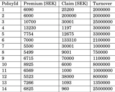
The method itself will be conducted on two different insurance products and their respective claim history. Further on the separated insurance portfolios will be referred to portfolio A and portfolio B. Now, each set of data follows the structure of a policy Id, premium, the loss amount and its policy’s characteristics. The insurance which is represented by portfolio A has its premiums based on the policyholders turnover and its chosen insurance amount where as insurance B is combined by several smaller insurance covers and therefore has ten different insurance amounts and the policyholder’s turnover as arguments for determine the premium. Our characteristic vectors are then seen as c_{A= (c1}, c₂) where c₁ corresponds to the turnover of the policyholder and c₂ the insurance amount. For cB= (c1, ..., c10) the first component is the turnover and the following are

several insurance amounts. The portfolios’ premium and loss vectors are referred to as P(c) and y(c). The structure of the data can be seen in the appendix where the two tables, A.1 and A.2, contains the two portfolios. Note that the insurances selected are the ones in the portfolio with claim history.

In the second part of the method and later on brought up for discussion is the application of the method on the entire portfolio. We will use the entire data set of Portfolio A, including the non-claim insurances, and with the help of the scoring function investigate its ordered Lorenz curve as well. The entire portfolio is constructed by 1321 different insurances and their corresponding characteristics. Unfortunately could the entire set of the non-claim insurances with its characteristics from Portfolio B not be retrieved from any database so the final analysis will only be conducted on Portfolio A.

CHAPTER 3. THE ORDER LORENZ CURVE METHOD

3.2

The Classic Lorenz Curve Method

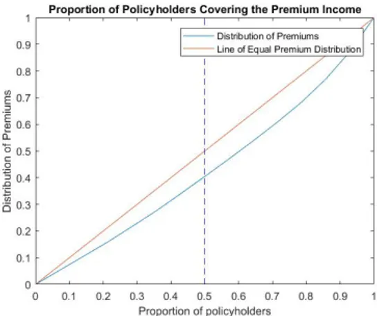
This section’s purpose is formulate the classic Lorenz curve in an insurance portfolio context. We study how the premium is distributed among the policyholders with only using the premium p as our sorting variable, following the structure of p_{i< pi+1< pn}. The empirical distribution for the premium is calculated according to

(3.1) FˆP remium(p) = Pn i=1PiI(Pi≤ p) Pn i=1Pi .

The classic Lorenz curve, "income versus people distribution", is then in terms of insurance business the premium distribution over the people. For the both portfolios the curve follows as below. Worth nothing is that portfolio B has a more evenly spread among their insurance premiums than portfolio A. Observing the lower 50th percentile of the policy holders, one sees that in Portfolio A they only cover almost 25% of the total premium while in Portfolio B it is closer to 40%.

Figure 3.1: Premium vs. Policyholder distribution of Portfolio A

Figure 3.2: Premium vs. Policyholder distribution of Portfolio B

3.3. SORTING CLAIMS AND PREMIUMS

3.3

Sorting Claims and Premiums

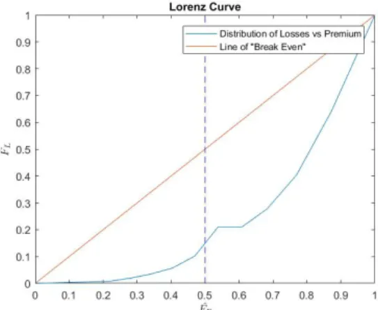
For each portfolio we let the claim be sorted as yi< yi+1. . . < yn and determine the empirical

distribution as (3.2) FˆL(s) = Pn i=1yiI( yi≤ s) Pn i=1yi .

combined with the sorted premiums in equation 3.1 we can then produce the loss and premium distribution in a graph for both portfolios.

Figure 3.3: Loss versus premium distribution of portfolio A

CHAPTER 3. THE ORDER LORENZ CURVE METHOD

3.4

Constructing the Ordered Relative Distributions

Begin by define the matrix which contains the characteristics of the insurance, cAand cB. The

matrix size correspond to the number of insurances included and the number of characteristics plus one. Remember that in 2.8 we also define_β0 and solve for it in 2.16, hence the characteristic matrix is extended with a column of ones, see 2.17. For the sake of not have to deal with large numbers which can affect the matrix calculations, we scale the characteristics by 106. Now, in portfolio A we have 16 insurances and 2 characteristics influencing the premium, for portfolio B the numbers are 14 and 10 making nA= 16, kA= 2 and nB= 14, kB= 10. Once the matrices

are defined the next step is to perform the regression analysis and determine the regression coefficients_β0. . .βk. Before we can determine the coefficients we need to determine the score S

based on our claims. As described in 2.6 we use the expected claim given the set of characteristics

c as our base for scoring. Based on the data given from portfolio A and B we can calculate the

expected claim as (3.3) _{S(c) = E[y|c] =}1 n n X i=1 yiI(ci= cj) ∀ j = 1...n.

Once the score is determined the relativity, here interpreted as a relative loss, can be calculated according to 2.18. There are several ways to define the relative variable R, but should be chosen such that it is clear to the user what the variable is intended to measure. In order to construct the ordered distributions for the premium and loss, the step variable r determine the distribution. Based on the relativity and its value from the characteristics, the empirical distribution functions

ˆ

Fp(s) and ˆFL(s) are now sorted on the same variable R(c).

(3.4) Fˆ_{P(r) =} Pn i=1P(ci) I(R(ci) ≤ r) Pn i=1P(ci) (3.5) FˆL(r) = Pn i=1yiI(R(ci) ≤ r) Pn i=1yi .

If we now plot the two ordered distributions against each other, they produce according to the theory section a valid ordered Lorenz curve which yield, from an analytic perspective, a deeper visual understanding of the portfolio’s performance rather than just the loss versus premium curve. To make distinguished comparisons between portfolios the Lorenz curve is well suited to the mathematics of the well established measure of difference between two distributions, the Gini index.

3.5. CALCULATE THE GINI INDEX

3.5

Calculate the Gini Index

As mentioned in the theory section, the Gini index can be interpreted as the area of which the Lorenz curve cover between the line of "break even" and the horizontal axis. In general theory the measure is coherent with spanning from (0,1). By the following extended definition of the Gini Coefficient we will let the measurement take the values between (-1,1), since it is a possibility that the portfolio is indeed underachieving. Since we are dealing with empirical functions, we cannot perform the theoretical measure 2.24, therefore we introduce the next step in the algorithm, the discrete Gini Coefficient. The discrete definition follows [5] deduction.

(3.6) G( ˆˆ FP, ˆFL) = 2 n−1 X i=1 ³ ˆ_{FP(i + 1) − ˆFP(i)}´³ ˆF_P(i + 1) + ˆF_P(i) 2 − ˆ F_{L(i + 1) + ˆ}F_L(i) 2 ´ (3.7) G( ˆˆ FP, ˆFL) = 1 − n−1 X i=1 ( ˆFP(i + 1) − ˆFP(i))( ˆFL(i + 1) + ˆFL(i))

C

4

R

The results and analytic value of the algorithm, performed on the two applied portfolios, will be presented in this section. Graphs from all three described Lorenz curves in the chapter regarding the method will be evaluated and the results from ordering the Lorenz curve by its relative will be presented. Furthermore, the results of the Gini index from corresponding graph are summarized and analyzed. If we recognize the stipulated aim of this report, one should remember that it is not the results of the digits which are of interest rather the results of the method’s application and what we intend to describe or measure.

4.1

Results of Portfolio A

Portfolio A contained 16 insurances with claim history and was described by its 2 characteristics, the turnover and the insurance amount. We begin by observing the graph 3.1 where the classical Lorenz curve is displayed with the premium as ordering variable. This figure is intend to give the observer a glance at the premium pricing distribution. What is relevant to notice is that the 50th-percentile of the people only covers roughly 25% of the premium, clearly the top 50% of the policyholders are covering the major part of the portfolios total income. Whether or not one can say that the results indicates that the likeliness of claim being more likely to occur for a policyholder with greater premium, since we only looking at the policies with existing claims in the entire portfolio, is not something that is evaluated by this method. Rather the result provides an easy understanding how this subset of this portfolio’s policyholders premiums are distributed.

The results from comparing the premium distribution with the loss distribution can be seen in the figure 3.3. The curve implies that the lower 50th percentile of the premiums covers around 35% of the total loss. Note that those policies which corresponds to the premiums are not connected

CHAPTER 4. RESULTS

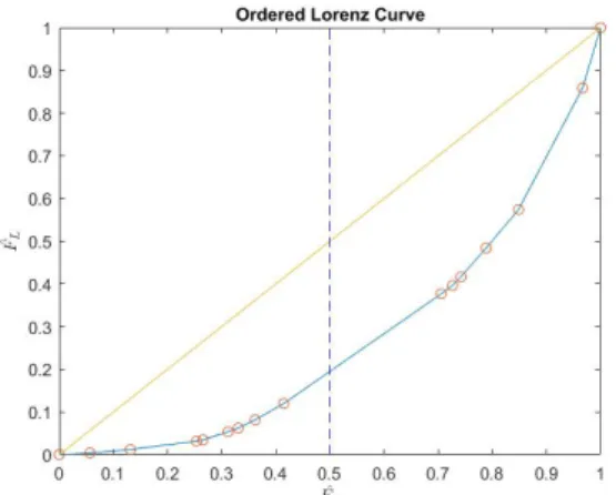
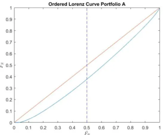
to the losses and therefore it is hard to reach any conclusion more than that the premium per policyholder in graph 3.1 where skewed to be top heavy while the premium versus losses seems to be more equal in distribution, therefore this Portfolio has greater variation in its losses. Further on, we study the results from the method of ordering the Lorenz curve by our relative variable. That is, our scoring variable the expected loss, divided by the policy’s premium. This graph 4.1 is presented below and results in the following. First, the result at the 50th lower percentile of the premium distribution covers only 20% of the losses. Here we see that, under the ordering of our relative loss, the portfolio is indeed top heavy. Second, the upper 5th-percentile covers the top 20% of the losses and compared to the 3.3 we see a much wider dispersion from the "line of equality". The losses and premiums are now connected through our relative variable which makes it easier to identify such insurances which puts a greater weight on the portfolio, hence we may construct a more profitable portfolio with these results.

Figure 4.1: Ordered Lorenz curve of portfolio A

Furthermore, the Gini index is calculated on all three graphs for assessment of the portfolio’s performance. As the figures are presented in table 4.1. Now, to compare the result from the classic Lorenz curve, that is the premium distribution versus the policyholders, with the two other does not provide much sense. However, the result of that Gini index will be of interest further on in the discussion between the two portfolio’s performance. When comparing the ordered Lorenz curve’s and the non-ordered’s Gini index there is a greater distinction between their results.

Premium vs. Policyholders Premium vs. Losses Ordered Lorenz Curve 39.38% 22.12% 46.16%

Table 4.1: The estimated Gini index for each of Portfolio A’s graphs

4.2. RESULTS OF PORTFOLIO B

4.2

Results of Portfolio B

The second portfolio which we performed the analysis on contained a set of 14 policies with each a corresponding claim. The policies for this portfolio was described by the ten characteristics

cB. With the classical approach and Lorenz curve, that is the policyholder versus the premium

distribution, the results in graph 3.2 visualize a portfolio with a flatter curve, closer to the line of even distribution. Comparing with Portfolio A, the result shows that for Portfolio B we see that about 50% of the lower percentiles of the policyholders cover 40% of the premiums. Observing the results from the graph 3.4 there is a larger dispersion from the line where we established even distribution between losses and premiums.

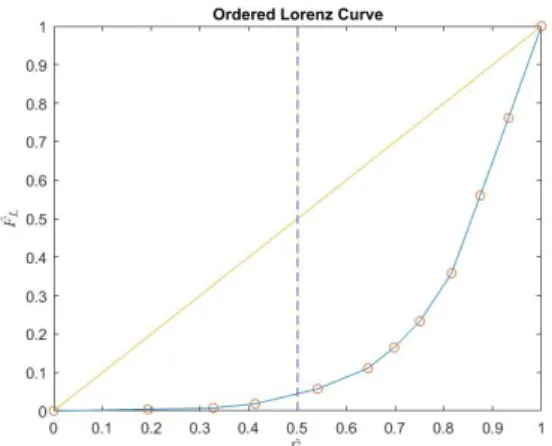
Now, the results show that the lower 50th percentile of the premiums cover 15% of the losses. However due to the sorting of the loss and premiums the result is not of further interest as described in the theory section. We continue by looking at the result that the ordered Lorenz curve yields. The curve is observed in the graph 4.2. The results show that by ordering through the set relative variable R(c) it yields a curve with a further attraction to the south east corner (1,0). The lower 50th percentile of the ordered premiums cover less than 10% of the losses. Furthermore, the Gini indices, which tells us something about the profitability of the portfolio, are evaluated as well for Portfolio B and visualized in table 4.2. As our empirical understanding of the curve tells us, the Gini index of the Ordered Lorenz curve shows a larger profitable segment of policies. With the result from both Portfolio A and B and their Gini indices, an analyst could now go ahead and compare and draw conclusions from their respective digits.

Figure 4.2: Ordered Lorenz curve of portfolio B

Premium vs. Policyholders Premium vs. Losses Ordered Lorenz Curve 14.71% 51.39% 64.57%

CHAPTER 4. RESULTS

4.3

Results of the Non-Claim Insurances in Portfolio A

With the regression coefficients determined, the insurances which had no previous claim his-tory could be rated. In the same procedure as before, the ordered Lorenz curve could then be determined based on its relative variable, i.e. 2.18. With its larger sample size, the distribution tends towards less dispersion from the line of equality and its lower 50th-percentile is now covering closer to 40% of the potential losses. While the curve is still below the line of equality this indicates a profitable portfolio and those insurances which are in the upper range could now be easier to locate and for an analyst perhaps re-structure the portfolio. Since we are looking at a portfolio with a sample of 1321 different insurances, this result indicated that refining the portfolio structure with the lower 70th-percentage of the premiums, which are related to 50% of the losses, would yield a profitable portfolio and lowering the risk of insurances with a higher relative loss. The Gini index, which can be seen in table 4.3 would in turn also be even higher with a re-structuring of the portfolio.

Figure 4.3: The ordered Lorenz curve of the entire portfolio A

Ordered Lorenz Curve 18.26%

Table 4.3: The estimated Gini index of the entire Portfolio A’s graph

C

5

D

This section intends to evaluate the theory, method and the results which was provided by the data. The underlying aim for this discussion is not to stipulate a formal conclusion for the application of this method, rather the text will be formulated in such way that the reader may comprehend the method and its abilities to lead them into thoughts for their own application and further development in the real world scenarios.

5.1

Discussing the Method and its Improvements

The theory behind the Lorenz curve is well established by economics and forms a basic intuition of any economical distribution relation one wish to examine. For an analyst in the insurance business the relation of premium and risk or losses would always be of interest. Are their relation in line with the strategy an insurer or broker has set up before covering such portfolios. Now, as a simple first step using the general Lorenz curve by observing the premium versus policy holder distributions, seen in graphs 3.1 and 3.2, they surely provides a basic understanding of how the portfolio’s premiums are distributed. One may discover fairly easy how Portfolio B’s premiums follows a more even distribution than Portfolio A. Likewise the following measure of the corresponding Gini index follow the understanding that the premiums in Portfolio B is distributed rather more evenly than Portfolio A with a much smaller figure, 0.1471 compared to 0.3134. Intuitively, the Gini measure for this case can be viewed as risk measure, rather than profitability as described for the Lorenz curve where one observe the premium versus losses. Hence the importance of understanding what one intend to describe. A portfolio structured similar to Portfolio B would be less sensitive to a drop or change of policyholders since their cumulative premium are closer to an even spread than Portfolio A, in which contrary will be more exposed to risk since the upper 50th percentage of policyholders carries a greater portion of the

CHAPTER 5. DISCUSSION

total premium in the portfolio. So the general Lorenz curve method does provide information but only with so much. Regarding relative exposure against losses the ordered Lorenz curve method provide deeper insight.

The method was based purely on observations and empirical distributions. Surely it is an easy and straight forward method but if one would dive deeper in the statistics of the method, a more theoretical approach would be of interest to ensure the statistical validity even further. Since data points are available an approach to assign a distribution to the random variable would be to observe the data points, fit a distribution which seems reasonable and with the use of a quantile-quantile plot, see [9], verify its validity. Once the distribution functions are known, the distributions could be plotted with its continuously curve and the insurance scoring could be better determined and statistically validated through confidence intervals.

Looking back at the intended purpose of this analysis, it was asked for a method which could identify specific block of policyholders based of their characteristics. Based on the order Lorenz curve method an insurance analyst can , based on the distribution be it the empirical or theoretical, identify the blocks of insurances which are above a set mark and re-balance the insurance portfolio with policyholders, having desired characteristics, and increase the profitability and reduce the risk of higher losses. For further analysis it is suggested to observe the characteristics which belongs to the insurances which are, according to the analyst performing well, and try to identify their treats and what separates them from the riskier ones.

5.2

The Scoring Function

Based on the data the theory showed that a scoring function, 2.8 could be determined based on solely a few data points. The scoring function 2.6 could be determined in several ways, but for this reports purpose of explaining the basics of a scoring function, a simple case of a linear function fulfills the criteria. Nevertheless, for the purpose of further develop a discussion of more elaborated approaches will follow in this section.

Now, this method elaborates only with the standard linear case. In some scenarios a rating plan is proposed but one would want re-think the characteristics which are suggested to be used when determine such a scoring function. A well known method to investigate the influence under ones measure is by its variable is the Principle Component Analysis. In short terms, this method seeks a maximize the variance and separation between groups and identify the driving variables, i.e. under which component tends the objects in the group be separated at most. With the use of Principle Component Analysis, an insurance analyst could use it to it advantage and reduce the number of characteristics being used in the scoring function. For further reading and explanation,

5.2. THE SCORING FUNCTION

see [3].

By evaluate the theoretical distribution of the data set, one could perform a regression analysis with a function closer in coherence with the theoretical distribution function for the losses. With the inclusion of the characteristics in the scoring function as variables. As an example, in [5] they determine the data of insurance losses to be of exponential distribution, hence assigning the scoring function to be exponential.

B

[1] URLhttps://it.wikipedia.org/wiki/File:Economics_Gini_coefficient.png.

[2] B. C. A. Albert W. Marshall, Ingram Olkin.

Inequalities: Theory of Majorization and Its Applications. Springer New York Dordedrecht Heidelberg London, 2011. [3] W. F. C. Alvin C. Rencher.

METHODS OF MULTIVARIATE ANALYSIS Third Edition. John Wiley Sons, Inc., Hoboken, New Jersey, 2012.

[4] C. W. . H. Best.

The SAGE Handbook of Regression Analysis and Causal Inference. SAGE Publications Ltd, 2013.

[5] A. D. C. Edward W. Frees, Glenn Meyers. Summarizing insurance scores using gini index.

Journal of the American Statistical Association, 106(495):1085–1098, 2011. [6] A. D. C. Edward W. Frees, Glenn Meyers.

Insurance ratemaking and a gini index.

The Journal of Risk and Insurance, 81(4):335–366, 2014. [7] J. L. Gastwirth.

A General Definition of the Lorenz Curve. The Econometric Society, 1971.

[8] J. L. Gastwirth.

The estimation of the lorenz curve and gini index.

The Review of Economics and Statistics, 54:306–316, 1972. [9] O. H. C. J. R. Henrik Hult, Filip Lindskog.

Risk and Portfolio Analysis, Principles and Methods. Springer Science+Business Media New York, 2012.

BIBLIOGRAPHY

[10] E. S. Shlomo Yitzhaki.

The Gini Methodology, A Primer on a Statistical Methodology. Springer New York Heidelberg Dordrecht London, 2013.

A

A

A

A

PolicyId Premium [SEK] Claim [SEK] Turnover [SEK] Insurance Amount [SEK] 1 10082 102003 54000000 5000000 2 3014 107500 1700000 5000000 3 3711 735313 2000000 10000000 4 3761 468433 170000000 10000000 5 9134 508750 30000000 10000000 6 7531 100000 24000000 10000000 7 3087 1480000 2000000 5000000 8 11360 43750 150000000 10000000 9 15500 350000 16400000 10000000 10 12516 826524 347207000 10000000 11 2983 15000 1156000 5000000 12 19462 100000 288000000 20000000 13 16762 200000 94627000 20000000 14 8619 100000 141172000 10000000 15 7429 20100 34000000 5000000 16 7958 42375 12700000 10000000

APPENDIX A. APPENDIX A

PolicyId Premium [SEK] Claim [SEK] Turnover 1 6090 25200 2000000 2 6000 200000 2000000 3 10700 30001 25000000 4 13230 1197 3000000 5 7754 12675 3300000 6 7000 133310 2100000 7 5500 30001 1000000 8 5499 9001 750000 9 6715 70000 1100000 10 8925 6000 8000000 11 6569 1000 10000000 12 5523 38000 800000 13 7266 1093 1350000 14 6825 960 25000000

Table A.2: Insurance portfolio B

PolicyId 1 2 3 4 5 6 7 8 9 10 1 5 17 2 2 0,444 0,8 0,1 6,15 0 0 2 5 17 2 2 0,444 0,8 0,1 6,15 0 0 3 5,05 17 2 5 0,445 1 0,1 6,15 0 0 4 5,05 17 5 2 0,445 1,2 0,1 6,15 0,09 5,34 5 5,248 17 2 2 0,443 2,12 0,1 6,15 0,015 2 6 5 17 2 2 0,444 0,8 0,1 6,15 0 0 7 5 17 2 2 0,444 0,8 0,1 6,15 0 0 8 5,248 17 2 2 0,443 1,1 0,1 6,15 0,015 0 9 5,248 17 2 2 0,443 1,24 0,1 6,15 0,015 2 10 5 17 2 2 0,445 0,8 0,1 6,15 0,015 5 11 5 17 0 2 0,445 0,8 0,1 6,15 0,015 0 12 5,196 17 2 2 0,445 1,12 0,1 6,15 0,015 0 13 0 17 5 2 0,445 0 0 6,15 0 0 14 5,05 17 2 2 0,445 1 0,1 6,15 0 0 Table A.3: Insurance portfolio B, insurance amounts in MSEK

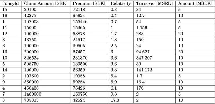
PolicyId Claim Amount [SEK] Premium [SEK] Relativity Turnover [MSEK] Amount [MSEK] 15 20100 72118 0.3 34 5 16 42375 95624 0.4 12.7 10 1 102003 155446 0.7 54 5 11 15000 15365 1 1.156 5 12 100000 58878 1.7 288 20 8 43750 24517 1.8 150 10 6 100000 39505 2.5 24 10 13 200000 67457 3 94.627 20 10 826524 231370 3.6 347.207 10 5 508750 139500 3.6 30 10 14 100000 26359 3.8 141.172 10 2 107500 19958 5.4 1.7 5 9 350000 59254 5.9 16.4 10 4 468433 76426 6.1 170 10 7 1480000 150756 9.8 2 5 3 735313 42524 17.3 2 10

Table A.4: Portfolio A ordered by the relativity variable

PolicyId Score Premium Relativity Turnover 1 2 3 4 5 6 7 8 9 10

4 1197 13230 0.1 3 5.05 17 5 2 0.445 1.2 0.1 6.15 0.090 5.34 14 960 6825 0.1 25 5.05 17 2 2 0.445 10 0.1 6.15 0 0 13 1093 7266 0.2 1.35 0 17 5 2 0.445 0 0 6.15 0 0 11 1000 6569 0.2 10 5 17 0 2 0.455 0.8 0.1 6.15 0.015 0 10 6000 8925 0.7 8 5 17 2 2 0.455 0.8 0.1 6.15 0.015 0.5 5 12675 7754 1.6 3.3 5.248 17 2 2 0.443 2.12 0.1 6.15 0.15 2 8 9001 5499 1.6 0.75 5.248 17 2 2 0.443 1.1 0.1 6.15 0.015 0 3 30001 10700 2.8 25 5.05 17 2 5 0.445 10 0.1 6.15 0 0 7 30001 5500 5.5 1 5 17 2 2 0.444 0.8 0.1 6.15 0 0 12 38000 5523 6.9 0.8 5.196 17 2 2 0.455 1.12 0.1 6.15 0.015 0 9 70000 6715 10.4 1.1 5.248 17 2 2 0.443 1.24 0.1 6.15 0.015 2 1 112600 6090 18.5 2 5 17 2 2 0.444 0.8 0.1 6.15 0 0 2 112600 6000 18.8 2 5 17 2 2 0.444 0.8 0.1 6.15 0 0 6 133310 7000 19 2.1 5 17 2 2 0.444 0.8 0.1 6.15 0 0

Table A.5: Portfolio B ordered by the relativity variable. The insurance amounts and turnovers are in MSEK while the Score and Premium are in SEK

TRITA -SCI-GRU 2019:372