Income
Inequality and
Economic Growth
BACHELOR
THESIS WITHIN: Economics NUMBER OF CREDITS: 15 ECTS PROGRAMME OF STUDY: International Economics and Policy
AUTHOR: Barbara Kandek and Veronika Kajling
JÖNKÖPING May 2017
What relation does regional inequality have with local
economic growth in US metropolitan areas?
Bachelor Thesis in Economics
Title: Income Inequality and Economic Growth Authors: Barbara Kandek and Veronika Kajling
Tutors: Charlotta Mellander and Emma Lappi Date: May 2017
Key terms: gini index, income inequality, economic growth, regional economics, united states
Abstract
Income inequality has been widely debated since the beginning of economic development. This topic is especially present in today’s economic world as the gap between the poor and rich only seem to widen, even in developed nations. Surprisingly, this is especially true for the United States where the top 1 percent own almost 50 percent of the nation’s income shares. Several studies have spoken on the impact inequality has on a nation, but few have commented on the effect it may have on a nation’s economic growth. Therefore, this paper aims to examine what relationship exists between regional inequality and local economic growth in 357 metropolitan cities in America. With the data gathered from the U.S. Census Bureau and several other databases, between the years 2010 and 2015, a series of OLS regressions are run. It is important to note research on the impact of income inequality on economic growth is few and far between, primarily on the city level due to data limitations. Thus, this disposition further contributes within the field of regional economics. The results in this paper, when regressing Gini to GDP Per Capita Growth and GDP Per Capita level, show Gini has a positive and significant relationship with GDP Per Capita Growth versus a negative and insignificant relationship with GDP Per Capita level.
Table of Contents
1. Introduction ... 1
1.1 Purpose ... 2
1.2 Disposition ... 3
2. Theories and Concepts ... 3
2.1 Theories on Income Inequality: Does Harm Growth ... 3
2.2 Theories on Income Inequality: Does Not Harm Growth ... 5
2.3 Regional Inequality in the United States ... 7
2.4 What Causes Cities to Grow? ... 9
3. Hypotheses and Expected Results ... 11
4. Methodology and Data ... 12
4.1 Empirical Model ... 12 4.2 Variables ... 12 4.2.1 Dependent Variables ... 12 4.2.2 Independent Variables ... 14 4.3 Econometric Method ... 16 5. Empirical Results ... 16 5.1 Descriptive Statistics ... 16 5.2 Correlation Analysis ... 17 5.3 Regression Analysis ... 18 6. Analysis of Results ... 20 7. Conclusion ... 24 8. Bibliography ... 26 9. Appendix ... 28
Tables
Table 1: Variables, Definitions, and Expected Signs ... 11
Table 2: Descriptive Statistics ... 16
Table 3: GDP Correlations ... 17
Table 4: Regression Equations GDP Growth ... 18
Table 5: Regression Equations Initial GDP ... 18
Table 6: Standardized Beta Values Initial GDP ... 28
Table 7: Standardized Beta Values GDP Growth ... 28
Table 8: Correlation Matrix ... 29
Figures
Figure 1: Scatterplot GDP Growth ... 13Figure 2: Scatterplot GDP Initial ... 14
Figure 3: Histogram Standardized Residual GDP Initial ... 30
Figure 4: Histogram Standardized Residual GDP Growth ... 30
Figure 5: P-P Plot of Standardized Residuals GDP Initial ... 31
1. Introduction
Income inequality has been a pressing issue since the development of nations. From ancient Greek philosophers to our now current politicians, income inequality and its impact has been widely debated. According to a report published by the IMF, “Widening income inequality is the defining challenge of our time. In advanced economies, the gap between the rich and poor is at its highest level in decades” (IMF 2015). Despite being highly developed, some Western nations have seen a steady increase in inequality in their own backyards. This is especially evident in the United States. As Alesina and Glaeser (2004) have found, America is relatively unequal for a developed country. Piketty and Saez (2003) highlight this further by researching how wealthy the richest 1 percent truly are in America; findings presented the 1 percent’s share of income rose by almost 14 percent just between 1979 and 2007.
In the next two years, from 2007 to 2009, the Great Recession took precedence over the United States. Americans experienced a long list of consequences due to the crash, from high unemployment rates, plummeting housing prices, and a labor market downturn (Fairlie 2013). The average real income declined by almost 18 percent during this time period (Saez 2013). For the top percentile, their average real income fell by 36.3%. The bottom 99 percent experienced a smaller fall of 11.6 percent, although the drop more than erased their 6.8 percent income gain from 2002 to 2007. After the recession, an uneven recovery occurred among Americans. The top percentile grew at a steady 11.2 percent while the bottom percentile shrunk by 0.4 percent. Despite the fall of income in the beginning of the crash, as households recovered, income inequality grew once again where in 2011, the top decile share equaled to 46.5%, the ‘highest ever since 1917’ (Saez 2013).
The recession highlighted the sharp inequality many Americans face today and how the recovery impacted households differently. Sampson (2016) argues inequality in America comes hand in hand with the ‘hollowing out of the middle class, stagnation of wages, and lack of upward mobility’. American individuals are now born and stuck in neighborhoods that are highly unequal, leading to a concentration of poverty, violence, and poor school quality at a regional level that, in the long term, creates a nationwide impact. Glaeser
(2009) believes local inequality is important to study, for crime rates are higher in unequal American cities and people are unhappier, leading to a higher possibility of political and social uprisings.
Panizza (1999) joins the debate on income inequality by finding channels linking inequality to economic growth. There exists many mixed theories and beliefs on how, if at all, income inequality and economic growth relate. Nevertheless, Panizza argues that political instability, imperfect capital markets, and redistribution pressure could be a reasoning behind a negative relationship. Nissan (2001) also studies the connection between inequality and economic growth by researching U.S. states, labeling his theory as ‘convergence’. This occurs when the income of regions approaches each other in the long run, thus the gap between the poor and the rich would also decrease. Nissan finds per capita personal income has shown to diverge during the 1980s despite a long-term tendency of convergence. Introducing growth into the equation, Nissan (2001) theorizes a reason for this change could be towards the disparate growth rates due to some central cities in the 1980s experiencing faster growth in their economies than others.
From poverty, violence, and lack of opportunity, the socioeconomic impact of income inequality can be debilitating in the development of a nation and its people. As Chernick et al. (2011) argues, one fifth of Americans live in the 100 largest cities in the nation. Thus, the growth and prosperity of cities are the key to the economic prosperity of a nation. This begins with furthering equality, so all Americans have the same opportunities and rights to better not only their situation, but the nation’s.
1.1 Purpose
The aim of this paper is to study what type of relationship exists between regional income inequality and local economic growth in 357 metropolitan cities in the United States. The time frame is a short-term of five years, specifically 2010 to 2015, which are also known as the recovery years after the Great Recession.
It is important to note there lacks specific research in this area, primarily when studying at the regional metropolitan level. This is due to a collection of factors, one of them being a limitation to data. Therefore, this paper contributes to the field of regional economics,
by studying if there exists a positive, negative, or no relationship with regional income inequality and local economic growth.
1.2 Disposition
This paper is organized as follows, Section 2 reviews the previous theories and concepts regarding income inequality. Section 3 shares the hypotheses tested in this paper. Section 4 presents the data, variables, empirical models, and methods. The empirical results are presented in Section 5, which are then analysed and discussed in section 6. Section 7 concludes the paper and provides suggestions for future research regarding the relationship between regional income inequality and local economic growth.
2. Theories and Concepts
In this section, existing theories on income inequality and its relationship with economic growth will be discussed. Concepts on both regional income inequality and local economic growth will follow.
2.1 Theories on Income Inequality: Does Harm Growth
Stiglitz (2012) argues inequality slows economic growth. According to Stiglitz, inequality weakens aggregate demand for individuals at the bottom and thus they spend a bigger portion of their income than those at the top. This makes sense intuitively; the poor often need to spend all their earnings simply to have the necessities to get by. Furthermore, Stiglitz argues the policy responses to fight weak demand can damage the economy. If monetary authorities decrease the interest rates, this can fuel bubbles that, upon bursting, may lead to a recession. Inequality of outcomes is linked with inequality of opportunity, thereby preventing individuals from low socio-economic backgrounds to reach their full potential. This indicates that income inequality has a negative effect even on future economic growth, putting families at risk of ending up in a poverty trap. Stiglitz points to rent seeking, when the rich seek to increase their own wealth rather than creating new wealth, as another important factor on how inequality can harm growth.
Much of the theoretical literature on inequality’s effect on growth presents imperfect capital markets, pressure for redistribution, and socio-political instability as plausible causes for a negative association between income inequality and economic growth.
Aghion et al. (1999) argues that inequality is harmful for growth in the presence of imperfect capital markets. If a functioning credit market is lacking, investments will depend on an individual’s own income and assets. The poor population may therefore not make any or enough investments that will raise their human capital. This is evident in the lack of investment in education within poorer communities. These poor individuals have higher marginal returns to investments than the wealthy. Hence, there is a potential for higher return on investment through redistribution. Imperfect capital markets can prevent the poor from educating themselves and their children, start businesses and afford insurances. These factors prevent the country itself from reaching the growth potential it might have faced with a more equitable distribution.
OECD (2014) finds a significant, negative relationship between inequality and economic growth in the OECD countries over a time span of 30 years. The gap between low income households and the remaining population was shown to be of greatest importance, while no evidence was found that the rich pulling away from the rest of the population harms growth. Their study revealed that in unequal societies, the poor invested less in their education and skills, while it barely had any impact on human capital investments among the middle and upper class. Hence, this implies that inequality will create an increasing education and earnings gap. The study divided the population into three different groups based on parents’ educational background (high, medium, low) and looked at numeracy scores within the three groups based on the OECD’s Adult Skills Survey. In unequal societies, the individuals from low socioeconomic background scored worse than they did in more equal societies. This can be considered economically inefficient, because a more skilled labour force can make greater contributions to the economy (Cingano, 2014). Persson & Tabellini (1994) discuss how conflict concerning the degree of distribution is likely to result in policies that impede growth. Economic growth takes place through accumulation of capital, human capital, and knowledge that is needed in production. Being able to appropriate the rewards of one’s efforts is important to incentivise individuals, thus redistribution policies risk distorting these motivations. Perotti (1996) refers to this as the fiscal policy approach with two different mechanisms. Equal societies demanding less redistribution (the political mechanism) results in lower levels of taxation, higher levels of investment, and growth (the economic mechanism). The fiscal policy approach implies a distinction between democracies and non-democracies. In democratic
societies, political outcomes are likely to reflect the wishes of the median voter. If inequality reaches high levels, the income of the median voter will be lower than the mean income of the economy. This creates a pressure for distributional policy actions. However, in a country that lacks a majority voting system, the fiscal policy approach does not predict any direct relationship between income inequality and growth.
Alesina & Perotti (1993) find that unequal societies are more politically unstable. Inequality causes social discontent, which in turn increases the degree of socio-political instability in a society. This unstable political and economic environment is harmful for economic growth by reducing investment, threatening property rights, and causing a larger number of coups and revolutions. Kelly (2000) considers the relationship between inequality and crime using data from urban counties in the United States, showing that inequality has an impact on violent crime. In a society with high inequality, the poor is faced with higher pressure and incentives to commit crime. An individual is more likely to turn to crime if they can expect a higher return from criminal activities than legal activities. In addition, when the rich become increasingly richer, the return of burglary is expected to increase (Chiu & Madden 1998).
A report from IMF has focused on the medium and long-term, analysing the growth rate over five-year periods through panel growth regressions and the length of growth spells. Their results show, for a given level of redistribution, lower net inequality is associated with faster and more robust growth. Furthermore, their research found a mostly benign effect of income distribution on growth. The IMF paper emphasises on the important distinction between market and net inequality. Net inequality is the inequality that prevails after taxes and transfers has been taking place. Hence, the inequality in disposable income. This distinction is important to make, for most countries differ more in terms of net inequality due to their varying distributional policies. In fact, because of these policies, there is almost no overall correlation between market and net inequality in the OECD countries (Ostry et al. 2014).
2.2 Theories on Income Inequality: Does Not Harm Growth
In neoclassical economics, there exists a trade-off between equality and efficiency. This is discussed by Okun (1975), he exemplifies transfers from rich to the poor as a “leaky bucket” were some money will be lost as it carried in the leaky bucket. Equality is
expected to affect incentives, and politicians must make a choice in whether to prioritize equity or economic efficiency. Kaldor’s (1955) reasoning for this trade-off is that the rich have a higher marginal propensity to save than the poor do. If one assumes that GDP growth has a direct relationship with the savings rate, this implies that unequal economies will experience faster growth. Furthermore, it implies that income redistribution, such as progressive taxation, will reduce the savings rate of the whole economy.
Another argument for how income inequality can be growth-enhancing, concerns the large costs involved in making investments, such as setting up new industries and implementing innovations. If wealth is more concentrated, at least some individuals have the sufficient resources to bring forward new investments (Aghion, et al. 1999). Mirrlees (1971) discusses the incentives concerning inequality and growth. In his model, output is dependent on unobservable effort borne by agents. If these agents are all rewarded with the same wage level, which is independent of their output, this will discourage an individual from putting in any additional effort. Hence, some inequality may be a necessity to foster growth and encourage productivity. Galor & Tsiddon (1997) claim that rising levels of inequality is observed during time periods characterized by major technological inventions. By improved mobility and a concentration of high-skilled workers in high-tech sectors, greater technological progress and growth will follow. Forbes (2000) finds a positive relationship between income inequality and growth in the short and medium run. This suggests that a trade-off between reducing inequality and improving a country’s growth performance may exist. Forbes questions some of the previous work which have found a negative relationship, claiming that they are likely to contain econometric problems such as measurement error and omitted-variable bias. Forbes’ work focuses on a shorter relationship within individual countries and she uses a panel estimation which enables control for time-invariant country-specific effects. Barro (1999) does not find any relationship between income inequality and growth. However, after dividing his sample into poor and rich countries, he finds a negative correlation for poor countries and a positive correlation for rich countries. He witnessed that in countries with a high initial level of GDP per capita (above $2000), the Gini coefficient exhibited a positive relationship with the growth of GDP. These results can
justify distributional policies in poor countries, whereas in rich countries redistribution might involve a trade-off with reduced economic growth.
Benhabib (2003) believes that the relationship between inequality and economic growth is in fact non-linear, proposing a “mildly hump-shaped” relationship. He argues that excessive inequality is disruptive of growth because it leads to rent-seeking while modest inequality boosts productivity. When inequality increases from low levels, it will have an enhancing effect on growth. However, past a certain point, inequality will start being harmful for growth. Hasanov & Izraeli (2011) also finds a non-linear, hump-shaped relationship between inequality and growth using data for 48 U.S. states over the time span 1960 to 2000. Their results suggest that stable inequality can be beneficial for growth, whereas both lowered inequality or a substantial increase can hurt growth performance.
2.3 Regional Inequality in the United States
Economic research on inequality has primarily focused on country level impact while studies on regional level inequality is few and far between. Reasoning behind this focus lies on the belief that convergence within cities and regions are less plausible, for institutional variables tend to equalize themselves in different regions over time (Nissan 2001). Panizza argues the comparison of regions actually offers a better and more controlled environment than of countries. This is primarily due to regional data being of ‘good quality and easily comparable across states’ (Panizza 1999). Sampson (2016) believes researching inequality at neighborhood and city level in the United States is fundamental in understanding the nationwide impact. Concentrated poverty, violence, and poor school quality tend to cluster together at neighborhood levels which harm the essential American notion. Upward contextual mobility is known to be the American Dream; individuals can triumph over their circumstances, such as growing up poor, and move to better neighborhoods which can give them better life opportunities (Sampson 2016). Glaeser supports the usage of studying regional level inequality from a more theoretical viewpoint. He believes local inequality is important to study for it has its own severity on a region. Crime rates are higher in more unequal cities and its individuals are less happy. The connection between crime and inequality is just as strong within urban areas as it is across countries (Glaeser 2009). These factors can easily generate political
uprisings, one of the elements that can harm both economic growth and income equality across not only nations but cities.
America is relatively unequal for a developed country, although specific areas in the states are more unequal than others (Glaeser 2009). While national inequality might hold constant, local inequality falls as people spread across spaces, specifically due to the fact the rich tend to live with the rich and poor with poor. Clearly this does not depict a better income distribution, if anything it is a skewed example. A perfectly integrated society, where the poor and rich are evenly distributed across spaces, would have highly unequal metropolitan areas that mirror better the country’s entire income distribution (Glaeser 2009). Glaeser found cities with both many college graduates and high school dropouts are areas that are particularly unequal. He discovered historical skill patterns play a huge role in the current location of college graduates, which could explain the current distribution of skills across regions. Generally, skilled people move to areas which have a larger return. As further studies show, places with more unequal skills grow quicker whereas areas with higher income inequality, while holding skills constant, have a slower income and population growth.
Eeckhout et al (2014) finds larger cities attract a disproportionate fraction of households from both the bottom and top of the income distribution. In one of his later papers, Glaeser further this belief by focusing on the concentration of the poor in American cities. His study finds that the poor live closer to the city center than the rich, primarily due to easy access to public transportation (Glaeser 2011). In 2011, suburbs had around 7.5 percent of the population living in poverty compared to 19 percent in central cities in America. A primary reason for this big difference is due to the large financial costs of automobiles which make it unattractive to lower income citizens. Behrens et al. (2014) focuses on the top of the income distribution by hypothesizing large cities attract rich households because of the higher returns to skills. This is deemed as the ‘superstar effect’ in ‘superstar cities’. There exists a tough selection process in cities which increase the returns to skills and earning inequality. The promise of better return incentives urban migration, causing an increase in more productive firms leading to large market shares and the ability to pay higher wages. While this seems like a positive occurrence, there is a negative side to the ‘superstar effect’ that mimics the survival of the fittest. Cities disproportionately reward the most skilled people while failing the least skilled. This occurs by cities offering
incentives for the most able to self-select employment options which offer high payoffs but the risk of failure increases because workers begin to compete against not only more, but better rivals. This unequal reward systems drives income inequality (Behrens et al. 2014.)
2.4 What Causes Cities to Grow?
The OECD (2015) claims that ‘productivity is the most important determinant of economic success’. This implies that to a great extent, the factors that determine productivity helps predict growth. When studying a metro area’s GDP growth one need to examine what affects the productivity of the metro. Different sectors in the economy do not have the same levels of productivity. Certain sectors generate a large amount of value added per worker, while other sectors generate relatively less value per worker. Thus, the composition of sectors within the metro’s economy plays an important role in determining its productivity and growth. Cities that are specialized in sectors that provide high levels of value added per worker, typically information technology, finance, and advanced manufacturing, is expected to achieve higher GDP per capita growth. However, for a city’s long-term growth, the ability to adapt and transform itself might be of greater importance, since sectors tend to mature and decline over time.
One important determinant of a city’s productivity is its levels of human capital. The highly educated on average display higher productivity, as reflected by their higher wages. Furthermore, they raise the productivity levels of the less educated. Moretti (2004) studies human capital spillovers, finding that plants in cities with a large stock of human capital are more productive compared to similar plants in smaller cities with less human capital. By increasing the share of university educated with ten percentage points, the productivity of those without university education was shown to increase with 5-6%. Florida (2003) suggest an extension of the human capital theory, that he refers to as the creative capital theory, identifying creative people as the key to economic growth. According to Florida, the three 3Ts – technology, talent, and tolerance – needs to be present in order for a place to attract these creative people, innovate and better its economic performance.
A report from Brookings (2013) discusses the importance of patenting and innovation as one of the driving force behind regional economic growth. Higher levels of patenting are
associated with greater productivity, more public corporations, and less unemployment. The authors point to research universities, a workforce educated in science and collaboration as important factors for driving the innovation of metros. They measure economic development in terms of economic output per worker and use control variables such as population, industry, housing prices and human capital, concluding that innovation seem to be a cause of growth.
The positive connection between growth and accumulation of human capital mentioned earlier implies a connection between a city’s size and growth. This could be due to large cities attracting more human capital and having a higher share of educated workers, argues the OECD (2015). Moreover, there are other agglomeration benefits suggesting a positive relation between growth and population size. A person migrating to a larger city is on average more productive there, this goes for both low- and high-skilled workers. A larger city has a larger labor market, making successful matching between employees and employer more likely. A person looking for a job can find a position that more closely matches his/her capabilities, hence the increased productivity. Investments involving large fixed costs might only be beneficial if many firms can ripe the benefits of it. Larger cities enable shared facilities and a greater degree of specialization. Furthermore, the existence of technology spillovers benefits larger cities. Businesses can exchange knowledge with and imitate each other. On the other hand, the presence of many firms increases competition within the city, which can incentivize higher productivity and innovativeness. Another benefit of being a larger metro is that it might be less vulnerable to sector-specific shocks (OECD, 2015).
Connecting the growth and development of a city with inequality brings us to the hypothesis of Kuznets (1955). Illustrated by an inverted U-curve, Kuznets’ theorizes in the early stages of development, inequality will first begin increasing. As a nation undergoes industrialization, cities will grow in importance and urbanization takes place. People working in agriculture will migrate to urban areas in order to find a job offering a higher income. Inequality increases due to a growing gap between an urban, high-productivity sector and a rural, low-high-productivity, and low-wage sector. Eventually, inequality tends to decrease as many have transitioned to the modern, high-productivity sector.
3. Hypotheses and Expected Results
The literature depicts conflicting predictions on the Gini coefficient’s effect on a country’s GDP per capita growth and the expected sign is ambiguous. Forbes (2000) studies a short-term relationship of five-year periods for the growth of GDP per capita. Since our paper is also looking at a five-year period, a positive relationship can be expected. Furthermore, this is in line with Barro’s (1999) finding that rich countries exhibit a positive relation between the Gini coefficient and GDP per capita growth. All the metros are classified as rich according to Barro’s definition. This leads to our first hypothesis:
H1: The Gini Coefficient displays a positive relationship with GDP per capita growth Our second hypothesis concerns how inequality have affected the level GDP per capita in 2010. Kuznets (1955) theorizes how inequality changes throughout a country’s phases of development. As an economy develops, inequality will initially rise but as the economy becomes more developed, inequality starts to decrease. According to the theory of the Kuznets curve, we would therefore expect metros with a lower Gini coefficient to be richer and more developed.
H2: The Gini Coefficient displays a negative relationship with GDP level
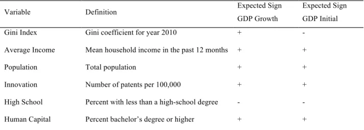
Table 1 summarizes the expected findings for our regression analysis, including the control variables.
Table 1: Variables, Definitions, and Expected Signs
Variable Definition Expected Sign
GDP Growth
Expected Sign GDP Initial
Gini Index Gini coefficient for year 2010 + -
Average Income Mean household income in the past 12 months + +
Population Total population + +
Innovation Number of patents per 100,000 + +
High School Percent with less than a high-school degree - - Human Capital Percent bachelor’s degree or higher + +
Crime Rates Number of violent crimes per 100,000 - -
4. Methodology and Data
In this section, the empirical model, variables, and econometric method are presented.
4.1 Empirical Model
The aim of this paper is to study the relationship between regional income inequality and local economic growth in 357 metropolitan areas in the United States. Based on the theoretical framework and previous research, the following models have been developed and, later, estimated with an OLS regression in Section 5:
(1) 𝑌 = 𝛽%𝐺 + 𝑙𝑔𝛽*𝐼 + 𝑙𝑔𝛽,𝑃𝑜𝑝 + 𝑙𝑔𝛽0𝑃 + 𝑙𝑔𝛽1𝐻𝑆 + 𝛽4𝐻𝐶 + 𝛽6𝐶𝑅 + 𝜀9 (2) 𝑋 = 𝛽%𝐺 + 𝑙𝑔𝛽*𝐼 + 𝑙𝑔𝛽0𝑃𝑜𝑝 + 𝑙𝑔𝛽0𝑃 + 𝑙𝑔𝛽0𝐻𝑆 + 𝛽*𝐻𝐶 + 𝛽0𝐶𝑅 + 𝜀9 where 𝑌 = 𝐺𝐷𝑃 𝐺𝑟𝑜𝑤𝑡ℎ 𝑋 = GDP Level 𝐺 = 𝐺𝑖𝑛𝑖 𝐼𝑛𝑑𝑒𝑥 𝐼 = 𝐴𝑣𝑒𝑟𝑎𝑔𝑒 𝐼𝑛𝑐𝑜𝑚𝑒 𝑃𝑜𝑝 = 𝑇𝑜𝑡𝑎𝑙 𝑃𝑜𝑝𝑢𝑙𝑎𝑡𝑖𝑜𝑛 𝑃 = 𝐼𝑛𝑛𝑜𝑣𝑎𝑡𝑖𝑜𝑛 𝐻𝑆 = 𝐻𝑖𝑔ℎ 𝑆𝑐ℎ𝑜𝑜𝑙 𝐻𝐶 = 𝐻𝑢𝑚𝑎𝑛 𝐶𝑎𝑝𝑖𝑡𝑎𝑙 𝐶𝑅 = 𝐶𝑟𝑖𝑚𝑒 𝑅𝑎𝑡𝑒𝑠 4.2 Variables 4.2.1 Dependent Variables
GDP Growth is expressed through the growth rate of GDP per capita of 2010 and 2015
in 357 metropolitan areas in the USA. This is calculated by subtracting the GDP of 2010 from 2015, then dividing it by the GDP of 2010. The data has been gathered from the U.S. Bureau of Economic Analysis (2015).
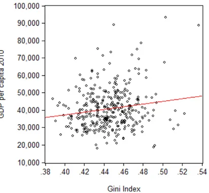
Figure 1: Scatterplot GDP Growth
Figure 1 presents GDP Growth and the Gini in a scatterplot. The fitted line between GDP per capita growth and Gini is close to flat, indicating there lacks a strong relationship between inequality and the growth for U.S. metros between the years 2010 and 2015. Most cities have slow growth rates, clustering below the 2 percent rate, while most cities are below 0.5 in the Gini Index range. An extreme outlier is Midland, Texas with a GDP growth of 65 percent and a Gini coefficient 0.5.
GDP Level is expressed through the growth rate of GDP per capita of 2010 in 357
metropolitan areas in the USA. The data has been gathered from the U.S. Bureau of Economic Analysis (2015).
Figure 2: Scatterplot GDP Initial
Figure 2, below, is a scatterplot showing the relationship between the variables, GDP Level and Gini. In this case, the data points are less clustered as with GDP growth. It appears, more unequal metros, on average, exhibit a higher level of GDP. Some of the metros with the highest levels of GDP in 2010, also exhibit some of the highest Gini coefficients. Midland, Texas is once again an outlier, the region has both the highest level of initial GDP and the highest GDP growth. It is the 8th most unequal metro in the United States.
4.2.2 Independent Variables
Gini Index is defined in Gini coefficients of 357 metropolitan cities in 2010. Values lie
between 0 and 1, where 0 signals ‘perfect equality’ and 1 signals ‘perfect inequality’. Data has been collected through the U.S. Census Bureau’s American Community Survey
from their 5-year estimate, 2006 to 2010.
Average Income is presented as the logged mean household income for the past 12
months in 2010. Data has been collected through the U.S. Census Bureau’s American Community Survey from their 5-year estimate, 2006 to 2010. An individual with high productivity is expected to earn a higher average income. Thus, metros with higher
average household incomes are predicted to be more productive and exhibit a higher GDP per capita growth.
Total Population is presented as the logged total population of 357 metropolitan cities in
2010. Data has been collected through the U.S. Census Bureau’s American Community Survey from their 5-year estimate, 2006 to 2010. Metros with a large population can ripe agglomeration benefits and they tend to attract a greater share of human capital, thus we expect a growing population size to have a positive relation with GDP per capita growth.
Innovation measures the amount of utility patents granted per 100,000 inhabitants in 357
metropolitan cities in the year 2010. The data is collected from U.S. Patent and Trademark Office (2010). An innovative, creative population is important for growing cities in today’s knowledge economy. Thus, we expect a positive relationship between the number of patents and the GDP per capita growth of a metro.
High School is measured as a percentage of the total population, between the ages of 18
and 24, with anything less than a high school diploma and is a proxy of the metros’ high school dropout rate and socioeconomic status. If a metro has a population with low levels of education, we expect less growth since human capital is suggested as an important factor for growth in much of the theoretical literature. Low socioeconomic status could also have other growth stunting effect such as poorer health. Data has been collected through the U.S. Census Bureau’s American Community Survey from their 5-year estimate, 2006 to 2010.
Human Capital focuses on the educational attainment in American cities. This is
measured as a percentage of the total population with, at the least, a bachelor’s degree in 2010, 25 years and older. Data has been collected through the U.S. Census Bureau’s
American Community Survey from their 5-year estimate, 2006 to 2010. A highly-educated population is expected to have a positive relation with growth, as education can rise an individual’s own productivity but also the productivity of others with lower education levels through human capital spillovers, as discussed by Moretti (2004).
Crime Rates measures violent crime rates per 100,000 inhabitants in 357 metropolitan
high level of crime in a metro is expected to be disruptive of growth by causing more social and political unrest.
4.3 Econometric Method
Changes in regional income inequality between 2010 and 2015 is examined over 375 metropolitan cities in the United States using a regression analysis. All independent variables are constructed with data from 2010 and the dependent variables show the change between the years 2010 and 2015. Thus, this paper uses cross-sectional data. When plotting the data, all variables show a liner relationship with the dependent variables. Therefore, an ordinary least square regression analysis is suitable.
A residual analysis has been performed to study whether the residuals in the model will impact the validity of the results given. Both independent variables appear to be normally distributed (Figure 3 and 4, Appendix), therefore no issues with heteroscedasticity are found.
5. Empirical Results
In this section, the findings of this paper will be presented. First, descriptive statistics and correlations are discussed, then the outcomes of the regression analysis will be presented.
5.1 Descriptive Statistics
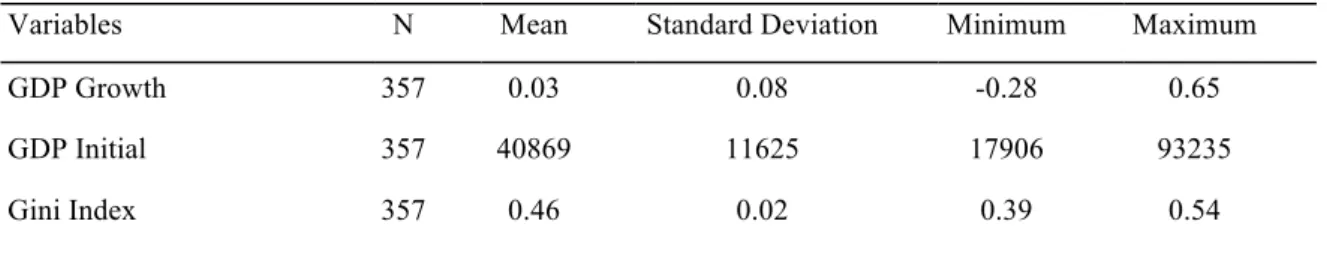
Table 2 provides descriptive statistics for the dependent and independent variables. As seen below, the mean value for the Gini Index is 0.46. This is a significant distance from the perfect equality standard of 0. GDP per capita’s mean value averages at around 50,000 US dollars. There seems to be a wide variation in GDP Growth, where the maximum value is 65% and the lowest being -28%. However, the mean value for GDP averages to about 3%. The remaining independent variables aim to explain any other variations in the dependent variables.
Table 2: Descriptive Statistics
Variables N Mean Standard Deviation Minimum Maximum
GDP Growth 357 0.03 0.08 -0.28 0.65
GDP Initial 357 40869 11625 17906 93235
Average Income 357 64214 11005 45141 130074 Population 357 704180 1575080 55375 1.87e+07 Innovation 357 28.27 48.82 0.41 561.57 High School 357 0.17 0.06 0.02 0.37 Human Capital 357 0.25 0.08 0.12 0.57 Crime Rates 318 372.14 164.39 53.40 1057 5.2 Correlation Analysis
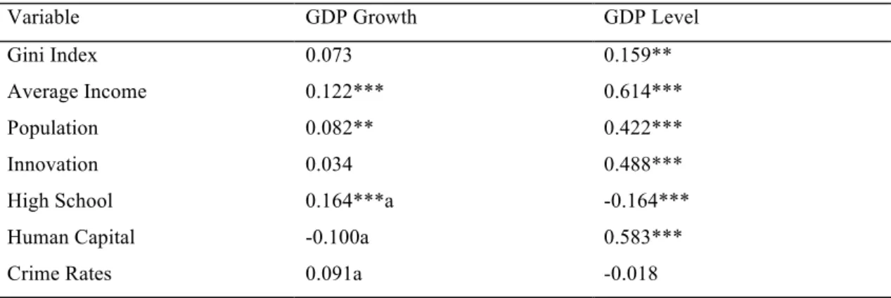
Table 3 displays the results of the bivariate analysis between the dependent variables and each independent variable. For GDP per capita growth, three variables are significant in a single regression analysis – average income, population and the rate of the population who are lacking a high-school degree. Gini Index, Innovation, Human Capital and Crime Rates do not show any statistically significant bivariate correlation. The High School variable and Crime Rates show signs which are conflicting with theory. For GDP Level, all variables except Crime Rates are significant. Gini Index at the 5% level, and the remaining at the 1% level.
Table 3: GDP Correlations
Variable GDP Growth GDP Level
Gini Index 0.073 0.159**
Average Income 0.122*** 0.614***
Population 0.082** 0.422***
Innovation 0.034 0.488***
High School 0.164***a -0.164***
Human Capital -0.100a 0.583***
Crime Rates 0.091a -0.018
*** Significant at 1% level ** Significant at 5% level a, variable show conflicting sign
Some of the independent variables are correlated with each other, as seen in (Table 8, Appendix). This indicates a potential problem of multicollinearity. Human Capital is highly correlated with several of the other regressors, particularly Innovation (0.678) and
Average Income (0.605). Thus, the highly educated are expected to have higher wages
and file for more patents. Human capital also exhibits quite a strong negative correlation with the High School variable (-0.546). Apart from Human Capital, Average Income is
correlated with both Innovation (0.534) and Population (0.474). Indicating that people in more populous metros, on average, have a higher income.
5.3 Regression Analysis
To study what extent income inequality and the controlled variables relate to GDP Growth and GDP Level in 357 metropolitan cities, an OLS regressions is run. Based on the F-statistics, all regression equations are significant at a 1 percent level. The results from the regressions are summarized in Table 4 and Table 5.
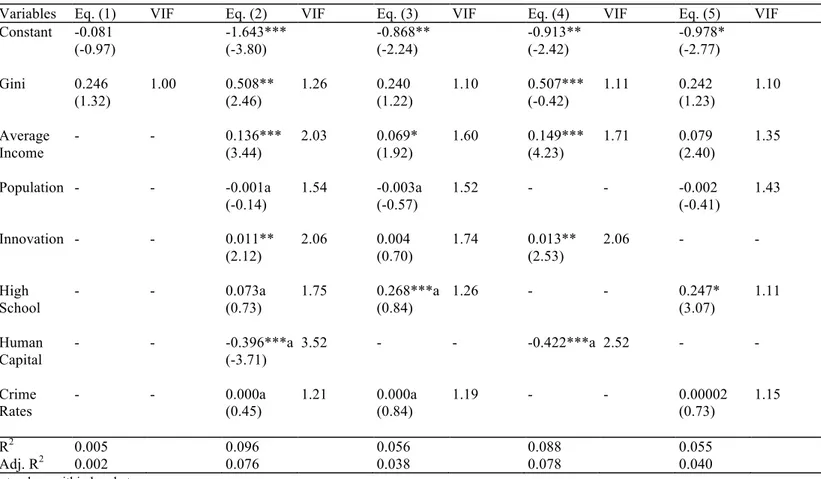
Table 4: GDP Growth Regression
Variables Eq. (1) VIF Eq. (2) VIF Eq. (3) VIF Eq. (4) VIF Eq. (5) VIF Constant -0.081 (-0.97) -1.643*** (-3.80) -0.868** (-2.24) -0.913** (-2.42) -0.978* (-2.77) Gini 0.246 (1.32) 1.00 0.508** (2.46) 1.26 0.240 (1.22) 1.10 0.507*** (-0.42) 1.11 0.242 (1.23) 1.10 Average Income - - 0.136*** (3.44) 2.03 0.069* (1.92) 1.60 0.149*** (4.23) 1.71 0.079 (2.40) 1.35 Population - - -0.001a (-0.14) 1.54 -0.003a (-0.57) 1.52 - - -0.002 (-0.41) 1.43 Innovation - - 0.011** (2.12) 2.06 0.004 (0.70) 1.74 0.013** (2.53) 2.06 - - High School - - 0.073a (0.73) 1.75 0.268***a (0.84) 1.26 - - 0.247* (3.07) 1.11 Human Capital - - -0.396***a (-3.71) 3.52 - - -0.422***a 2.52 - - Crime Rates - - 0.000a (0.45) 1.21 0.000a (0.84) 1.19 - - 0.00002 (0.73) 1.15 R2 0.005 0.096 0.056 0.088 0.055 Adj. R2 0.002 0.076 0.038 0.078 0.040
t-values within brackets ***Significant at 1% level. ** Significant at 5% level. * Significant at 1% level. a, variable show conflicting sign
Equation 1 examines GDP Growth and Gini. The model has an adjusted R2 of 0.002. Gini has a beta coefficient of 0.246, thus a 1 unit increase in GDP Growth leads to a 0.246 unit increase in Gini. However, Gini is insignificant with GDP Growth when running a simple bivariate analysis. Thus, we cannot state there exists a relationship between the two variables when excluding all other independent variables.
Equation 2 examines GDP Growth including all independent variables. The model has an adjusted R2 of 0.076. Gini is significant at the 5 percent level and is positive, indicating that as GDP per capita growth rises, so does inequality. If the control variables are fixed, then for each one unit increase in GDP per capita growth, the Gini coefficient increases by 0.508 units. This is in line with the expected results. The variables Average Income,
Innovation, and Human Capital are significant. The High School variable, although
insignificant, exhibits a positive sign which conflicts with theory. In this case, the model presents the opposite expectation; as the number of citizens with less than high school education grow, growth will follow and increase as well. The first equation faces a risk of multicollinearity issues, particularly the Human Capital variable, which shows a relatively high VIF value of 3.52.
Equation 3 examines GDP Growth including all independent variables but Human
Capital, due to not only a high VIF value but its high correlation with other variables as
detailed in Section 5.2. The model has an adjusted R2 of 0.038. Gini remains positive but becomes insignificant with the dependent variable. Meaning, we can no longer detect any statistically significant linear dependence between GDP per capita growth and inequality.
Innovation is no longer significant at the 1 percent level and instead is significant at the
10 percent level. High School becomes highly significant and continues to display a positive relationship with growth, despite expectations.
Equation 4 examines GDP Growth including all independent variables that were significant in the bivariate analysis. The model has an adjusted R2 of 0.078. This is a higher adjusted R2 than in equation 1, which could indicate that some of the variables do not add much explanatory power to the regression. In equation 3, the Gini Index is highly significant and positive in relation with GDP Growth. Average Income and Innovation are also highly significant and display positive relationships with our growth variable.
Human Capital becomes an outlier in this case, although significant there seems to be a
negative relationship with growth, which conflicts with the aforementioned theories and concepts.
Equation 5 excludes both Human Capital and Innovation to avoid multicollinearity at the fullest degree. These two variables are correlated with each other, as highly educated people are expected to innovate more. Furthermore, they are both correlated with Average
have a high correlation with each other which can be further explained in the correlation matrix (Table 8, Appendix). In this equation, only High School shows a statistical significance in explaining growth.
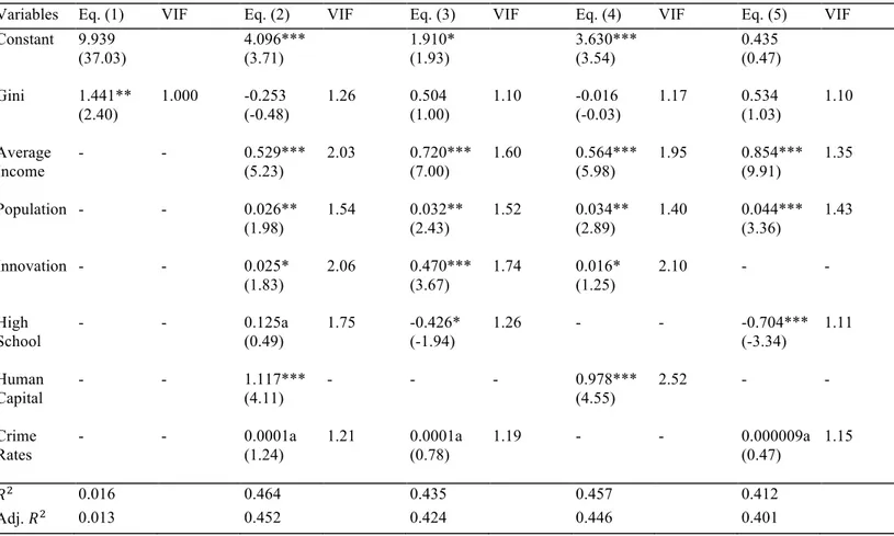
Table 5: GDP Level Regression
Variables Eq. (1) VIF Eq. (2) VIF Eq. (3) VIF Eq. (4) VIF Eq. (5) VIF Constant 9.939 (37.03) 4.096*** (3.71) 1.910* (1.93) 3.630*** (3.54) 0.435 (0.47) Gini 1.441** (2.40) 1.000 -0.253 (-0.48) 1.26 0.504 (1.00) 1.10 -0.016 (-0.03) 1.17 0.534 (1.03) 1.10 Average Income - - 0.529*** (5.23) 2.03 0.720*** (7.00) 1.60 0.564*** (5.98) 1.95 0.854*** (9.91) 1.35 Population - - 0.026** (1.98) 1.54 0.032** (2.43) 1.52 0.034** (2.89) 1.40 0.044*** (3.36) 1.43 Innovation - - 0.025* (1.83) 2.06 0.470*** (3.67) 1.74 0.016* (1.25) 2.10 - - High School - - 0.125a (0.49) 1.75 -0.426* (-1.94) 1.26 - - -0.704*** (-3.34) 1.11 Human Capital - - 1.117*** (4.11) - - - 0.978*** (4.55) 2.52 - - Crime Rates - - 0.0001a (1.24) 1.21 0.0001a (0.78) 1.19 - - 0.000009a (0.47) 1.15 𝑅* 0.016 0.464 0.435 0.457 0.412 Adj. 𝑅* 0.013 0.452 0.424 0.446 0.401
t-values within brackets ***Significant at 1% level. **Significant at 5% level. *Significant at 10% level. a, variable show conflicting sign
Equation 1 examines GDP Level with Gini. The model has an adjusted 𝑅* of 0.013 and a
beta coefficient of 1.441. This implies that a 1 unit increase in GDP Level will lead to a 1.441 unit increase in Gini. In this simple bivariate analysis, Gini is significant at the 5 percent level. Thus, we can assume there exists a significant relationship between GDP
Level and Gini when all other independent variables are excluded.
Equation 2 examines GDP Level including all independent variables, the model has an adjusted 𝑅* of 0.452. Gini shows a negative but insignificant relationship with growth.
Thus, we cannot prove that there is any linear dependency between inequality and a metro’s level of GDP per capita. Crime Rates and High School are insignificant as well. The former exhibiting a negative relationship and the latter a positive relationship, both
of which contradict the theoretical framework. The only variables that are significant at a 1 percent level are Human Capital and Average Income, while Innovation and Population are significant at the higher levels. The VIF values are almost all below 2.0, this could be interpreted as there being no existing multicollinearity. As mentioned in our correlation analysis, there are variables that exhibit strong correlations with each other. One of the variables with the highest correlations is Human Capital, which could be giving us biased results.
Equation 3 examines GDP Level including all independent variables except Human
Capital due to high correlations with other variables. In this model, the adjusted 𝑅* is
0.424. The only insignificant variables are Gini and Crime Rates, although Gini now shows a positive relationship with Growth. By excluding Human Capital, Innovation becomes highly significant at the 1 percent level. High School shares a negative relationship with growth and is significant at the 10 percent level. VIF values have become a small fraction lower when excluding Human Capital, decreasing the risk of multicollinearity.
Equation 4 examines GDP Level with all independent variables that were significant in the bivariate analysis, including Gini. Gini is insignificant, but continues to have a negative relation with GDP Level as in Equation 1. This indicates that the more unequal a metro, the lower the level of GDP per capita. However, due to the lack of statistical significance we cannot prove that any relation between inequality and GDP level exists. All other variables are significant and seem to follow the same relationships as from Equation 1.
Equation 5 excludes Human Capital and Innovation as they are highly correlated with each other. Furthermore, they also share high correlation with Average Income and High
School (Table 8, Appendix). Gini is positive with GDP per capita, but remains
insignificant as it has been throughout all the regressions. Our regression results tell us that inequality does not seem to be a statistically important factor in explaining a metro’s level of GDP per capita. Average Income and Population are both highly significant and positive. The High School variable is highly significant and negative, supporting our expected results in 3.
6. Analysis of Results
GDP GrowthWith GDP Growth as the dependent variable, the Gini coefficient exhibits a positive relationship with Gini, as proposed by our first hypothesis. However, the Gini coefficient is not significant in the regression model with human capital excluded (Equation 2, Table 4). The inclusion of human capital may have imposed a multicollinearity problem, and therefore the results should be interpreted with some caution.
The positive relationship between inequality and short-term growth is supported by previous empirical work. One explanation for the positive relationship is larger cities are more unequal (Eeckhout, 2014). As cities grow, they tend to attract a disproportionate fraction of households from both the bottom and top of the income distribution which aggravates inequality (Eeckhout, 2014). As discussed by Behrens et al. (2014) a superstar effect can also be observed, a tough selection process takes places which tend to excessively reward the most skilled people. Meanwhile, as discussed in section 2.4, large cities often grow faster as they ripe agglomeration benefits and attract a greater share of human capital (OECD 2015). Metros that highly rewards skills might, to a greater extent, have been able to attract the high-skilled population necessary to foster growth in today’s knowledge-based society. This is also known as the skill premium, which increases inequality (Behrens 2014).
The theory that large cities grow more proposes a linkage between economic growth and population. However, in our regression output, Population is an insignificant variable that shows a conflicting sign with theory. Furthermore, the sign of Human Capital is also conflicting with the theoretical framework, despite it being significant in the two equations where it is included. Average Income shows a positive sign and is significant throughout the three regressions, implying that metros with a higher average household income experienced more economic growth during the five-year period. The higher incomes may be reflected by a higher productivity of the metro’s inhabitants.
Another reasoning behind the positive relationship between inequality and growth is the possibility that the relationship is non-linear, as suggested by Benhabib (2003). Unequal metros in the U.S. may still be experiencing the growth-enhancing effects of inequality
and are located on the upswing of the hump-shaped curve. However, if inequality keeps rising past a certain threshold, the relationship may reverse due to an increase in behaviours like excessive rent-seeking.
Some scholars claim that inequality tends to increase while a place is experiencing technological progress (Galor & Tsiddon 1997). Technological progress could be one of the explanations for a positive relationship, since new technology increases productivity and thus helps growing the economy. Metros who have gone through technological progress may witness both an increase in their level of inequality and economic growth.
GDP Level
When running a regression analysis for the first equation, all explanatory variables included, we find Gini has a negative relationship with GDP Level. This contradicts the analysis when GDP Growth is used as the dependent variable, where the relationship is positive. Gini is also significant at the 5 percent level with GDP Growth but insignificant when run with GDP Level. Although the negative relationship correlates with our hypothesis, because Gini is insignificant we cannot reject nor accept the hypothesis. In all four regression analyses, the Gini coefficient remains insignificant throughout. This indicates that inequality does not explain a metro’s level of GDP per capita. Instead, the factors that seem to determine how rich a metro is are, primarily, Average Income and Human Capital. Both variables are significant and positive at the 1% level in the equations (when included). The connection with average income might be intuitive; if the metro’s households have a higher mean income, GDP per capita is expected to be higher as well. As discussed in section 2.4, human capital accumulation is an important factor in growing an economy (Moretti 2004). Population and Innovation are also significant and positive in the regression which implies, metros with a larger population and a greater number of patents per capita are, on average, richer. Despite Gini’s insignificance, it is interesting to consider why Gini has a negative relationship with the dependent variable and how the control explanatory variables fit in the discussion.
Stiglitz (2012) mentions a ‘poverty trap’ that occurs due to income inequality, where the inequality of outcomes is linked to the inequality of opportunities. If certain individuals are born in low income neighborhoods, they are less able or inclined to have as many
investments as one from a higher income background. This leads to lack of financial resources to provide better opportunities, such as the chance for higher education or to live in safer and wealthier neighborhoods. Stiglitz (2012) indicates this has a negative effect on future economic growth, primarily if ‘rent seeking’ is evident. This occurs when the rich are increasing their own wealth rather than creating new wealth, which causes the poor to be stagnant or ‘stuck’ in a poverty cycle.
Cingano (2014) observes income inequality and economic growth over 30 years, the findings show low income households invest less in their education and skills due to the need to spend the income they do own just to survive. This reasoning could explain a negative relationship between a metro’s GDP per capita and the Gini coefficient. A negative relationship would also be predicted by the Kuznets hypothesis, since inequality is expected to decrease throughout the course of economic development. However, worth noting is that the coefficient for the Gini Index not appear to be very robust as it shifts sign between the different equations, depending on what control variables are included. Due to its lack of robustness and significance, we cannot conclude that inequality plays a role in determining a metro’s wealth.
7. Conclusion
This paper has studied the relationship between economic growth and inequality on a regional level in the United States, by using data from 357 metropolitan statistical areas. The theories on income inequality’s effect on economic growth is highly debated and, more commonly than not, offers an ambiguous answer. Those proposing a negative relationship stress how inequality can hurt educational attainment among the poorer classes, cause a pressure for redistribution policies, result in socio-political instability and excessive rent-seeking. Scholars suggesting a positive relationship generally highlight the incentives provided by high rewards and technological progress, which give rise to both inequality and growth.
Our regression results point to the existence of a tradeoff between inequality and economic growth in the short run. However, the relationship is not strong and robust enough to justify political action. Most of the metros are scattered in a nearly straight line, thus many metros have grown at similar rates despite varying levels of inequality. The
Gini coefficient loses its significance in the regression equation when human capital is excluded. This might be the case due to the high correlations human capital has with other explanatory variables. Moreover, there is a limitation in the study because there is a lack of observation when it comes to how inequality changes over a longer period of time. Therefore, the study examines how growth changes in a city but not how inequality does over the years. In our cross-sectional study, we are not able to observe how a change in a metro’s level of inequality will affect growth within that metro.
When using the initial level of GDP in 2010 as the dependent variable, Gini never exhibits statistical significance. Gini also shifts signs, from negative to positive in the regression equation when Human Capital is excluded. Thus, the level of equality or lack thereof does not seem to be an important explanatory factor for regional economic growth in the United States. Other variables, such as Human Capital and Average Income, appears to be more important for the initial GDP level as it remains significant throughout the regression.
It is also important to note correlation does not imply causation. Despite Gini having a positive relationship with GDP Growth and a negative relationship with GDP level, this does not necessarily mean inequality is beneficial for growth. Factors that might motivate inequality, could also be ones that increase growth such as technological progress, an unequal skill distribution, and city size. To expand the study, suggestions such as different time spans and studying the changes in inequality could highlight further the impact on growth. In conclusion, further research is recommended in the field to gain more knowledge on the impact regional inequality might have on local economic growth.
8. Bibliography
Aghion, P., Caroli, E., & García-Peñalosa, C. (1999). Inequality and Economic Growth: The Perspective of the New Growth Theories. Journal of Economic Literature
Vol.37(4), 1615-1660.
Alesina, A., & Glaeser, E. (2004). Fighting Poverty in the US and Europe: A World of
Difference. Oxford: Oxford University Press.
Alesina, A., & Perotti, R. (1993). Income Distribution, Political Instability, and Investment. NBER Working Paper Series, 4486.
Barro, R. (1999). Inequality and Growth in a Panel of Countries. Journal of Economic
Growth Vol.5(1), 5-32.
Behrens, K., & Robert-‐Nicoud, F. (2014). Survival of the Fittest in Cities: Urbanisation and Inequality. Economic Journal Vol.124(581), 1371-1400.
Benhabib, J. (2003). The Tradeoff Between Inequality and Growth. Annals of Economics
and Finance Vol. 4(2), 491–507.
Chernick, H., Langley, A., & Reschovsky, A. (2011). The impact of the Great Recession and the housing crisis on the financing of America's largest cities. Regional
Science and Urban Economics Vol.41(4), 372-381.
Chiu, W., & Madden, P. (1998). Burglary and income inequality. Journal of Public
Economics Vol.69(1), 123-141.
Cingano, F. (2014). Trends in Income Inequality and its Impact on Economic Growth. Paris: OECD Publishing .
Eeckhout, J., Pinheiro, R., & Schmidheiny, K. (2014). Spatial Sorting. Journal of
Political Economy 122(3), 554-620.
Fairlie, R. (2013). Entrepreneurship, Economic Conditions, and the Great Recession.
Journal of Economics & Management Strategy Vol.22(2), 207-231.
Florida, R. (2003). The Rise of the Creative Class: And how It's Transforming Work,
Leisure, Community and Everyday Life. New York: Basic Books.
Forbes, K. (2000). A Reassessment of the Relationship Between Inequality and Growth.
The American Economic Review Vol.90(4), 869.
Galor, O., & Tsiddon, D. (1997). Technological Progress, Mobility, and Economic Growth. The American Economic Review Vol.87(3), 363.
Hasanov, F., & Izraeli, O. (2011). Income Inequality, Economic Growth, and the Distribution of Income Gains: Evidence from the U.S. States. Journal of Regional
Science Vol.51(3), 518-539.
Kaldor, N. (1955). Alternative Theories of Distribution. The Review of Economic Studies, 83-100.
Kalpana Kochhar, E. D.-N. (2015). Causes and Consequences of Income Inequality: A Global Perspective. IMF Staff Discussion Notes.
Kelly, M. (2000). Inequality and Crime. Review of Economics and Statistics Vol.82(4), 530-539.
Kuznets, S. (1955). Economic Growth and Income Inequality. The American Economic
Review Vol.45(1), 1-28.
Mirrlees, J. A. (1971). An Exploration in the Theory of Optimum Income Taxation. The
Review of Economic Studies Vol.38(2), 175-208.
Moretti, E. (2004). Workers' Education, Spillovers, and Productivity: Evidence from Plant-Level Production Functions. The American Economic Review Vol.94(3), 656-690.
Nissan, E., & Carter, G. (2001). Income Inequality in Large U.S. Cities in the 1980s.
Review of Urban & Regional Development Studies Vol.13(1), 62-72.
OECD. (2015). The Metropolitan Century: Understanding Urbanisation and its
Consequences. Paris: OECD Publishing .
Ostry, J., Berg, A., & Tsangarides, C. (2014). Redistribution, Inequality, and Growth.
IMF staff discussion note.
Panizza, U. (2002). Income Inequality and Economic Growth: Evidence from American Data. Journal of Economic Growth Vol.7(1), 25-41.
Perotti, R. (1996). Growth, income distribution, and democracy: What the data say.
Journal of Economic Growth Vol.1(2), 149-187.
Persson, T., & Tabellini, G. (1994). Is inequality harmful for growth? The American
Economic Review Vol.84(3), 600(22).
Piketty, T., & Saez, E. (2003). Income Inequality in the United States, 1913-1998. The
Quarterly Journal of Economics Vol.118(1), 1-39.
Rothwell, J., Lobo, J., Muro, M., & Strumsky, D. (2013). Patenting Prosperity: Invention
and Economic Performance in the United States and its Metropolitan Areas.
Washington: Brookings.
Saez, E. (2013). Striking it Richer: The Evolution of Top Incomes in the United States.
IDEAS Working Paper Series.
Sampson, R. (2016). Individual and Community Economic Mobility in the Great Recession Era: The Spatial Foundations of Persistent Inequality. Economic
Mobility: Research and Ideas on Strengthening Families, Communities and the Economy, 261-287.
Stiglitz, J. (2012). The Price of Inequality: How Today's Divided Society Endangers Our
9. Appendix
Table 6: Standardized Beta Values Initial GDP
Variables Eq. (1) Eq. (2) Eq. (3)
Gini -0.022 0.045 -0.152 Average Income 0.340 0.421 0.315 Population 0.102 0.128 0.135 Innovation 0.120 0.206 0.097 High School 0.027 -0.926 0.230 Human Capital 0.320 - 0.296 Crime Rates 0.056 0.036 - 𝑅* 0.464 0.435 0.454 Adj. 𝑅* 0.452 0.424 0.446
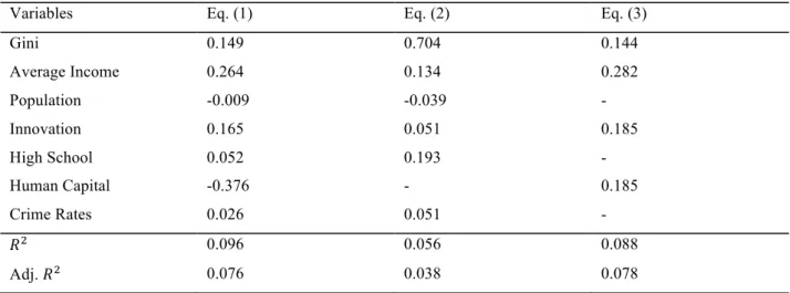
Table 7: Standardized Beta Values GDP Growth
Variables Eq. (1) Eq. (2) Eq. (3)
Gini 0.149 0.704 0.144 Average Income 0.264 0.134 0.282 Population -0.009 -0.039 - Innovation 0.165 0.051 0.185 High School 0.052 0.193 - Human Capital -0.376 - 0.185 Crime Rates 0.026 0.051 - 𝑅* 0.096 0.056 0.088 Adj. 𝑅* 0.076 0.038 0.078
Table 8: Correlation Matrix
Gini Index
Average Income
Population Innovation High School Human Capital Crime Rates Gini Index 1.000 Average Income 0.059 1.000 Population 0.223 0.474 1.000 Innovation 0.072 0.534 0.367 1.000 High School -0.055 -0.120 0.070 -0.360 1.000 Human Capital 0.276 0.605 0.363 0.678 -0.546 1.000 Crime Rates 0.209 -0.036 0.182 -0.190 0.248 -0.169 1.000
Figure 3: Histogram Standardized Residual GDP Initial
Figure 5: P-P Plot of Standardized Residuals GDP Initial