A study of turbulence and scalar mixing in a wall-jet using direct numerical simulation

(1)

A study of turbulence and scalar mixing in a

wall-jet using direct numerical simulation

by

Daniel Ahlman

April 2006 Technical Reports from Royal Institute of Technology

Department of Mechanics SE-100 44 Stockholm, Sweden

(2)

Akademisk avhandling som med tillst˚and av Kungliga Tekniska Högskolan i Stockholm framlägges till offentlig granskning för avläggande av teknologie licentiatexamen fredagen den 28 april 2006 kl 10.15 i D3, Huvudbyggnaden, Kungliga Tekniska Högskolan, Lindstedtsvägen 5, entréplan, Stockholm.

c

°Daniel Ahlman 2006

(3)

A study of turbulence and scalar mixing in a wall-jet

using direct numerical simulation

Daniel Ahlman

Dept. of Mechanics, Royal Institute of Technology SE-100 44 Stockholm, Sweden

Abstract

Direct numerical simulation is used to study the dynamics and mixing in a turbulent plane wall-jet. The investigation is undertaken in order to extend the knowledge base of the influence of the wall on turbulent dynamics and mixing. The mixing statistics produced can also be used to evaluate and de-velop models for mixing and combustion. In order to perform the simulations, a numerical code was developed. The code employs compact finite difference schemes, of high order, for spatial integration, and a low-storage Runge-Kutta method for the temporal integration. In the simulations performed the inlet based Reynolds and Mach numbers of the wall jet were Re = 2000 and M = 0.5, respectively. Above the jet a constant coflow of 10% of the inlet jet velocity was applied. A passive scalar was added at the inlet of the jet, in a non-premixed manner, enabling an investigation of the wall-jet mixing as well as the dynam-ics. The mean development and the respective self-similarity of the inner and outer shear layers were studied. Comparisons of properties in the shear layers of different character were performed by applying inner and outer scaling. The characteristics of the wall-jet was compared to what has been observed in other canonical shear flows. In the inner part of the jet, 0 6 y+₆_{13, the wall-jet was}

found to closely resemble a zero pressure gradient boundary layer. The outer layer was found to resemble a free plane jet. The downstream growth rate of the scalar was approximately equal to that of the streamwise velocity, in terms of the growth rate of the half-width. The scalar fluxes in the streamwise and wall-normal direction were found to be of comparable magnitude.

Descriptors: wall-jet, direct numerical simulation, turbulence, scalar mixing

(4)

Preface

In this thesis, dynamics and mixing in a plane wall-jet are studied by means of direct numerical simulation. In the following introduction, a brief background and the context of the work is presented. In the enclosed papers, the results and conclusions of the performed simulations are presented and the developed simulation code is documented. The thesis is based on and contains the follow-ing papers;

Paper 1. Ahlman D., Brethouwer G and Johansson A. V., 2006 “Direct numerical simulation of a plane turbulent wall-jet including scalar

mixing”, To be submitted

Paper 2. Ahlman D., Brethouwer G. and Johansson A. V., 2006 “A numerical method for simulation of turbulence and mixing in a compressible

wall-jet”, Technical Report, Dept. of Mechanics, KTH, Stockholm Sweden

(5)

Division of work between authors

The project was initiated and defined by Arne Johansson (AJ) and Geert Brethouwer (GB). The work was performed by Daniel Ahlman (DA) under the supervision of AJ and GB.

The simulation and computation of statistics in Paper 1 was performed by DA. The paper was written by DA and examined by GB and AJ.

The code development described in Paper 2 was performed by DA. The report was written by DA and examined by GB and AJ.

(6)

(7)

Som f¨or vindarnas v˚

ald ett moln f¨orsvinner,

som i klingande b¨ack en v˚

ag f¨orrinner

liks˚

a m¨anniskans dagar

rastl¨ost ila sin kos.

Erik Johan Stagnelius (1793–1823)

(8)

(9)

Part I

Introduction

(12)

CHAPTER 1

Introduction

1.1. Turbulence and combustion

One of the most prominent features of turbulent flows is the diffusivity. The turbulent flow state infers rapid mixing and transfer of fluid properties such as mass, momentum and heat. Turbulent mixing rates are significantly higher than mixing rates in laminar flows, where it occurs exclusively at the molecular level. In fact turbulent diffusivity is the reason why we stir our cup of coffee after adding milk, to quickly mix it evenly. Relying on the slow molecular mixing would leave us waiting till the coffee had cooled off.

The diffusivity of turbulence also has important implications in turbulent combustion. In technical applications such as automobile engines or gas tur-bines, combustion nearly always takes place in turbulent flow fields. The reason for this stems mainly from the fact that combustion is enhanced by the turbu-lence. For combustion, characterized by high rates of heat release, to occur, the participating species have to be mixed to the right proportions on the molec-ular level. The high rates of transport and mixing inherently present in the turbulent environment, generate a faster combustion and energy conversion rate. Combustion processes also include heat release, which through buoyancy and gas expansion can generate instabilities.

From this brief description it is evident that the combustion is strongly coupled to the turbulent flow field. Turbulence close to the flamefront may interact with the flame in a number of ways depending on the scale and strength of the turbulent fluctuation. Large, high intensity velocity fluctuations, may convolute the flame, increasing the flame surface and also the reaction rate. As the fluctuation scale becomes small and eventually of the order of the flame thickness it can enhance the mixing close to the flamefront but also quench the it locally through high strain.

The influence of combustion on turbulence, apart from the altered fluid dynamics due to density and temperature changes, is less prominent. However, when the temperature increases in the vicinity of the flame, owing to heat transfer from the reaction zone, the viscosity of the fluid increases and may locally modify the turbulence.

Gaseous turbulent combustion is subdivided into different r´egimes, describ-ing the species initial mixdescrib-ing situation. The reaction processes are described as premixed, non-premixed or partially premixed turbulent combustion. In the

(13)

1.1. TURBULENCE AND COMBUSTION 3 premixed r´egime the participating species are thought to be perfectly mixed before ignition. This is generally the case in spark-ignition engines, where the fuel and oxidizer are mixed by turbulence for sufficiently long time, prior to the spark ignition of the mixture. Premixed flames also possess an inherent flame speed. As the reaction progresses in the premixed r´egime, the flame propagates relative to the unburnt mixture.

When fuel and oxidizer enter the combustion chamber in separate streams prior to reaction, the combustion is instead termed non-premixed. The flames present in this combustion r´egime are commonly referred to as diffusion flames, indicating that diffusion processes are essential for bringing the fuel and oxi-dizer into contact. Contrary to flames in a premixed environment, diffusion flames do not possess an inherent flame speed. In aircraft turbines, the liquid fuel is injected into the combustion chamber. The liquid evaporates before it burns, typically in a non-premixed way in the form of diffusion flames. In-coming reactants from non-premixed streams must be continuously mixed and ignited by burnt gases, in order for the combustion to proceed. This process is referred to as flame stabilization and is often accomplished fluid dynamically by creating recirculation zones. Intermediate to these canonical r´egimes is par-tially premixed combustion. This occurs when fuel and oxidizer are injected separately but are able mix partially before ignition. This is generally speaking the case in diesel engines.

Combustion of fossil fuels globally constitutes the dominating source of en-ergy. Energy from other sources such as hydroelectric, solar, wind and nuclear energy account for less than 20% of the total energy consumption. Combus-tion of fossil fuel will therefore prevail as a key energy conversion technology at least in the next few decades. However, the negative environmental impacts of excessive fossil fuel combustion are becoming evident. Emissions of CO2

contribute to global warming. Other pollutants produced such as unburnt hy-drocarbons, soot and nitrogen oxides (NOx) have also been found to have a

negative impact on the environment. Nitrogen oxides in particular contribute to acidification, photochemical smog and influence the ozone balance in the stratosphere. More rigorous regulations concerning emissions are presently en-forced in the automotive industry and on power plants to reduce emissions and environmental impact. To reach these goals, an improved understanding of combustion and mixing processes is needed, as well as improved models to be used in the development of cleaner combustion applications.

The present thesis concerns the investigation of turbulent dynamics and mixing near a wall, by means of direct numerical simulation. The study is part of a long term project, with the aim of simulating combustion near cold solid walls. In the present work, simulations of passive scalar mixing in a turbulent plane wall-jet have been performed. Information of the underlying mixing pro-cesses is of importance for evaluation and development of combustion models. Since the wall-jet configuration contains a solid wall, a study of the wall in-fluence on the dynamics and mixing is facilitated. In the following sections,

(14)

4 1. INTRODUCTION

the interaction of the wall and turbulent combustion in the near-wall region is described. The role of numerical simulation in the study of combustion phe-nomena is outlined, and an overview of the area of combustion modeling is presented. In the section on modeling, the importance of accurately represent-ing the mixrepresent-ing situation is emphasized.

1.2. Mixing and combustion near walls

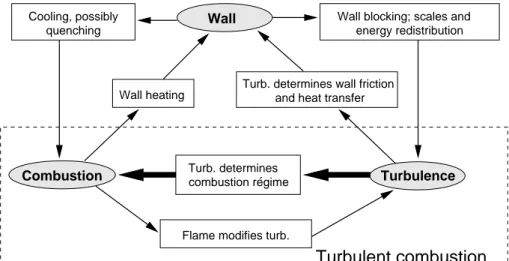
In order to generate power, combustion processes often take place in chambers. Inside a chamber, some of the reaction and mixing is likely to occur close to, and be affected by, the solid enclosing walls. In the near-wall area, the interaction of the wall and the turbulent combustion will be complex. These interactions are outlined in figure 1.1. Since the solid wall usually is significantly colder

Wall heating

Wall blocking; scales and energy redistribution Cooling, possibly

quenching

Turb. determines combustion regime

Turb. determines wall friction and heat transfer

Wall

Turbulence

Flame modifies turb.

Combustion

Turbulent combustion

Figure 1.1. The interaction between the wall and the turbu-lent combustion (modified from Poinsot & Veynante (2001)).

than the burning mixture, a heat flux is generated towards the wall. The wall thus cools the flames. This can lead to flame quenching. In internal combustion engines, flame wall interaction is one of the dominant sources of unburnt hydrocarbon emission. Another influence of the wall is on the mixing of the reacting components. Close to the wall turbulent fluctuations are damped, resulting in reduced mixing.

Clearly the wall influences the mixing and combustion in the vicinity of the wall in a profound way. It is therefore of interest to study processes in this region, and to add to the knowledge of the complex interaction. Simulations of mixing and combustion near walls are useful for a number of reasons. Accu-rate experiments in this region are difficult since the region of interest is very close to the wall. Highly resolved simulations can be used to support model development. Most combustion models are developed for isotropic conditions

(15)

1.3. THE ROLE OF SIMULATIONS 5 far from walls. It is not fully known how accurate the present models can cap-ture wall effects on the mixing and combustion. Considering that walls have a profound impact, it is of interest to evaluate and develop accurate mixing and combustion models for the near-wall region.

1.3. The role of simulations

Direct numerical simulations (DNS) has emerged as a valuable tool in the study of mixing and combustion phenomena. Increasing computational resources have facilitated high resolution simulations, but also simulation of more com-plex phenomena including coupled fluid dynamics and chemistry.

The benefit of DNS in investigations of mixing and combustion is that it provides access to the complete solution, because all length and time scales are resolved. Higher order statistics such as correlations, probability density func-tions and conditional averages can be computed. The largest disadvantage of DNS is the computational cost. Since all scales have to be resolved, simulation of engineering application is not possible. The range of scales present in these makes the simulation prohibitively computationally demanding, even for the foreseeable future.

For simulations of reacting flows, the description of the reactions also have to be simplified. A complete mechanism for the simple reaction of hydrogen and oxygen gas typically involves 19 reactions and 9 species (Conaire et al. 2004). The combustion of a primary reference fuel (PRF) of iso-octane and n-heptane, used to evaluate the octane number of gasoline, is described by a mechanism of 4238 reactions and 1034 species (Curran et al. 2002).

Considering the limitations, DNS should be regarded as a useful tool for model development and evaluation. Highly resolved simulations of simplified model problems can produce information on how to construct accurate mod-els, and can be used to test which model approach provides the most accurate prediction. Bilger (2000) presents an overview of the issues of current interest in turbulent combustion, including the status and outlook of present computa-tional models. The recent progress in the application of DNS to study premixed turbulent combustion is reviewed by Poinsot et al. (1996), and non-premixed combustion is reviewed by Vervisch & Poinsot (1998).

Using experiments, measurements of the complete reaction phenomena and in some cases directly in the technical application, are possible. Also experimen-tal techniques have exhibited a fast evolution. The advent of laser measurement technique has allowed for the development of fast and accurate measurement techniques. In comparison to simulation, experimental investigations however provide more localized information.

Studies of combustion near walls employing DNS include Poinsot et al. (1993) who studied flame-wall interaction of laminar and premixed combustion, through compressible two-dimensional DNS, using a simple reaction. Bruneaux et al. (1996) employed incompressible three-dimensional simulations of pre-mixed combustion in a channel using a simple reaction. They found that

(16)

6 1. INTRODUCTION

quenching distances decrease and maximum heat fluxes increase in compari-son to those of laminar flames. Their DNS data was also used in Bruneaux et al. (1997) to develop and evaluate a flame surface density model. Using a complex reaction mechanism consisting of 18 reactions involving 8 species, one-dimensional premixed and non-premixed flame interaction with an inert wall was simulated by Dabrieau et al. (2003). Wang & Trouv´e (2005) used DNS to study flame structure and extinction events of non-premixed flames interacting with a cold wall. Their simulation was fully compressible, two-dimensional and the reaction was described using a single step model containing four species.

1.4. Combustion models

Numerical computation of turbulent combustion is often divided into three categories in terms of the resolution of the computation. The highest level of resolution is reached by solving the governing equations without resorting to models, referred to as direct numerical simulation (DNS). The application of DNS to combustion was discussed in the previous section.

In large eddy simulation (LES) the large scales are resolved, while the smaller, unresolved scales, are modelled. By reducing the resolved range of scales the computational effort is also reduced. A review of the application of LES to combustion, and its modelling issues, is presented by Pitsch (2006).

The classical, and least computationally demanding approach, is to fully av-erage the governing equations. This introduces unclosed terms that have to be modelled. During the last decades, a wide variety of combustion models based on this approach have been developed. Some of the more prominent mod-els, presently used and still under development, include probability-density-function (pdf) models (Pope 1985), flamelet models (Peters (1971,2000)) and conditional moment closure methods (Klimenko & Bilger 1999). A recent overview of the state-of-the-art in combustion modeling has been published by Veynante & Vervisch (2002), but can also be found in Bilger (2000) and in the books of Poinsot & Veynante (2001) and Peters (2000).

1.4.1. Averaged conservation equations

Reacting flows in general include heat release, and therefore also significant density fluctuations. This has implications for the averaging of the governing equations. When averaging the conservation equations for constant density flows, Reynolds decomposition of the flow variables, into a mean ¯f and fluctu-ating f0_{component, is conventionally used. Applying this to flows with varying}

density introduces unclosed correlations involving the fluctuating density of the type ρ0_f0_{. To reduce the number of unclosed terms, mass-weighted averages,}

also called Favre averages, are usually employed. Favre decomposition of an instantaneous variable f is performed through

f = ρf_¯ f + f

(17)

1.4. COMBUSTION MODELS 7 where ef denotes the mass-weighted mean and f00the corresponding fluctuating part. Using this decomposition and formalism, the averaged equations for conservation of mass, momentum and the mass fractions θk= mk/m, of species

k = 1, . . . , N involved in the reaction becomes ∂ ¯ρ ∂t + ∂ ∂xi (¯ρeui) = 0 (1.2) ∂ ¯ρeui ∂t + ∂ ∂xj (¯ρeuieuj) = − ∂ ¯p ∂xi + ∂ ∂xj ³ ¯ τij− ρu00iu 00 j ´ (1.3) ∂ ¯ρeθk ∂t + ∂ ∂xi (¯ρeuiθek) = ∂ ∂xi µ ρDk ∂θk ∂xi − ρu 00 iθk00 ¶ + ˙ωk (1.4)

The Favre averaged equations are formally identical to the Reynolds averaged equations for constant density flows. The unclosed terms appearing in the equa-tions are the Reynolds stresses ρu00

iu00j, the scalar fluxes ρu00iθ00k and the reaction

source term ˙ωk. Closure for the Reynolds stress term is usually achieved with

a RANS-type turbulence model, e.g. a k–² model.

An often used model for the scalar flux is formulated in terms of a classical gradient diffusion assumption

ρu00 iθ00k = ¯ρ ]u00iθk00= − µt Sckt ∂ eθk ∂xi (1.5) where µtis the turbulent viscosity, estimated from the turbulence model, and

Sckt is the turbulent Schmidt number, which is usually of the order of one. In

the case of reactive flow a gradient based model is a poor approximation for a number of reasons. The model can be argued to fail at the reaction zone, where the reaction influences the scalar flux. Furthermore it is assumed that the scalar flux is aligned with the mean gradient, which in general is not true (Wikstr¨om et al. 2000).

Modeling the reaction source term ˙ωkcan be regarded as the key difficulty

in modeling turbulent combustion. The problem can be appreciated by study-ing the simple reaction F + O → P . The mean reaction rate of the Fuel species F is of the form

wF = −ρ2θFθOk = −ρ2θFθOBe(−Ea/RT ) (1.6) where k(T ) is the Arrhenius reaction rate constant and Eathe activation energy

of the reaction. The reaction rate is highly temperature dependent, which can have implications in computations in terms of stiffness of the solution. Also, the reaction rate is a function of the product of the instantaneous species concentrations, which can be termed as the mixing. In fact if the reaction rate is sufficiently fast, which it often is, the combustion rate depends directly on the mixing rate. The full expression is highly non-linear, indicating that modeling in terms of mean variables is not suitable.

(18)

8 1. INTRODUCTION

1.4.2. The eddy break up (EBU) model

An early attempt to model the mean reaction rate was proposed by Spald-ing (1971). In premixed combustion the model is formulated in terms of the progress variable c = (T − Tu)/(Tb− Tu), reaching from 0 in the unburnt (Tu)

to 1 in the completely burnt (Tb) mixture. Assuming that the reactions are

sufficiently fast, the turbulent mixing becomes the rate-determining process, and the reaction rate is modelled as

˙ω = ¯ρCEBU p f c002 τEBU = ¯ρCEBU ² k q f c002 _(1.7)

where CEBU is a model constant, τEBU is a characteristic time scale of the

reaction and c002 _{is the variance of the progress variable. Since fast reactions}

are assumed, the time scale is estimated to correspond to the integral time scale of the turbulent flow field τEBU = k/².

Also assuming that the flame is infinitely thin, the species can only take two values since it is either fresh or fully burnt. In this case the mean reaction rate can be written as

˙ω = ¯ρCEBU²

keck(1 − eck) (1.8)

in terms of the known mean quantities. Due to the simplicity of the description, the eddy break up model is found in most commercial combustion codes. The obvious limitation of the model however is that no effects of chemical kinetics is included.

1.4.3. Non-premixed combustion models

In order to provide an example of how passive scalars enter into models of combustion, examples from the the modeling of non-premixed combustion are also presented here.

Models of non-premixed combustion are usually derived using a set of sim-plifying assumptions. Typical assumptions include constant and equal heat capacities for all species, low Mach numbers and unit Lewis numbers. Employ-ing these assumptions, the flame position can be related to a scalar quantity, z, termed the mixture fraction. Using global conservation of species, linear combi-nations of the species and temperature, Zj, can be constructed that eliminates

the source terms. The scalars Zjare all governed by the same balance equation,

∂ρZ ∂t + ∂ ∂xi(ρuiZ) = ∂ ∂xi µ ρD∂ρZ_∂x i ¶ (1.9) when the diffusivity D has been assumed constant and equal for all species. Since the source term is eliminated, Z is a conserved scalar, subjected to dif-fusion and convection only. Reactions however plays an indirect role for the density and velocity fields by controlling the heat release. Normalization of the

(19)

1.4. COMBUSTION MODELS 9 variables Zj can be performed through

zj=

Zj− ZjO

ZF j − ZjO

(1.10) where superscript F denotes values in the fuel stream and O values in the oxidizer stream. The normalized variables zjare governed by the same balance

equation and subjected to the same boundary condition; zj = 1 in the fuel

stream and zj = 0 in the oxidizer stream. Hence all normalized variables are

equal, reducing the problem to the solution of one conserved scalar, the mixture fraction z.

In turbulent combustion models, the solution of the averaged mixture frac-tion is sought. Using Favre averaging this becomes

∂ ¯ρez ∂t + ∂ ∂xi(¯ρeuiz) =e ∂ ∂xi µ ρD_∂x∂z i − ¯ρ ]u 00 iz00 ¶ . (1.11)

In the averaged equation, the mixture fraction scalar flux ]u00

iz00is usually

mod-elled using a gradient diffusion assumption of the form in (1.5). This gradient assumption is more justified for the mixture fraction, since it is a conserved scalar.

The introduction of a mixture fraction is used in many models. The reason for this is that it provides a possibility to avoid the direct closure of the species source term, which was seen in section 1.4.1 to be a hard task. The definition of the mixture fraction can essentially be used to split the solution of the mean flame properties, the mixture fractions and the temperature, into two problems; a mixing problem and a flame structure problem. The first problem consists of describing the underlying mixing situation, which is provided from the mixture fraction. For an accurate description, both the mean field ez and higher order statistics, preferably the full pdf p(z), are needed. Usually at least the variance fz002 _{is provided. In the following flame structure problem,}

the flame properties, mass fractions, temperature and species source terms, are recovered by using the mixture fraction information i.e. the flame properties are expressed conditionally on the mixture fraction and its higher moments.

When the pdf of z, p(z) is known, the procedure to compute the average values, using the information of the underlying mixing can be expressed as

¯ ρeθk= Z 1 0 ³ ρθk|z∗ ´ p(z∗)dz∗, ρ e¯T = Z 1 0 ³ ρT |z∗´_p(z∗_)dz∗ _(1.12) ¯ ρ ˙ωk = Z 1 0 ³ ρ ˙ωk|z∗ ´ p(z∗_)dz∗_. _(1.13)

Here z∗ _{is used to represent the mixture fraction and its higher moments e.g.}

the scalar dissipation rate χ described in section 1.4.5. (f|z∗_{) denotes the}

conditional average of the quantity f for a set of mixture fraction statistics z = z∗_.

(20)

10 1. INTRODUCTION

As an example, using the flamelet model approach, the flame structure is characterized by the mixture fraction and the scalar dissipation rate at the reaction front χst. Flame structure functions of the form θk(z, χst) are

pre-calculated for laminar flames and stored in “flamelet libraries”. The averaged property can then be computed from

¯ ρ eθk= Z ∞ 0 Z 1 0 ρθk(z, χst)p(z, χst)dzdχst (1.14)

where p(z, χst) is the joint pdf of the mixture fraction and the scalar dissipation

rate at the reaction front.

1.4.4. Infinitely fast chemistry

In the limit of infinitely fast chemistry, the combustion is determined solely by the mixing. Moreover, since reaction is instant, the flame structure depends only on the mixture fraction z. The mean quantities can be computed as

¯ ρeθk= Z 1 0 ρθk(z)p(z)dz, ρ e¯T = Z 1 0 ρT (z)p(z)dz (1.15) The only unknown in the infinitely fast chemistry limit is thus p(z). The determination of the pdf of the mixture fraction in a reacting mixture is still an open question. Two possible routes are to either estimate the pdf using an assumed shape, or to solve a transport equation for the pdf (Pope 1985). For engineering purposes the first possibility is often sufficient. The most common assumed pdf is the β-function, which is defined as

p(z) = z

a−1_{(1 − z)}b−1

B(a, b) (1.16)

where B is a normalization function. The parameters a and b are determined from the mean ez and variance fz002 _{of the mixture fraction as}

a = ez µ e z(1 − ez) f z002 − 1 ¶ , b = a e z − a. (1.17)

The structure of the pdf and also the complete flame is defined through the assumed pdf. The determination of the pdf requires information of the mixture fraction ez and its variance fz002_.

1.4.5. Scalar variance transport equation

Most combustion models require information on a scalar variance for closure. As was seen in the previous section, even in the limit of infinitely fast reactions using an assumed pdf approach, information on the passive scalar variance z002

is needed.

Regarding the mixing information contained in the mixture fraction, the mean field value ez can be seen to represent the global location and the struc-ture of the flame. For information of the local mixing situation, higher order statistics are needed. The mixture fraction variance fz002_{provides the first level}

(21)

1.4. COMBUSTION MODELS 11 of information of the local mixing. The scalar variance can be employed di-rectly for closure in moment methods and in models employing assumed pdfs. In fact most higher level combustion models include assumed pdfs in their for-mulation. Both models using the flamelet approach, and conditional moment closure models include assumed pdfs.

In the RANS approach the variance is obtained from a transport equation. The transport equation for the mixture fraction variance fz00 _reads

∂ ¯ρ fz002 ∂t + ∂ ∂xi ³ ¯ ρeuizf002 ´ = −_∂x∂ i ³ ρu00 iz002 ´ | {z } I + ∂ ∂xi Ã ρD∂z 002 ∂xi ! | {z } II − 2ρu00 iz00 ∂ez ∂xi | {z } III − 2ρD∂z 00 ∂xi ∂z00 ∂xi | {z } IV (1.18)

when D is constant. The the various right hand side terms are identified as (I) turbulent transport, (II) molecular diffusion, (III) production and (IV ) dissi-pation. Closing the equation requires models for all the right-hand-side terms. For the turbulent transport, a gradient transport model of the form in (1.5) can be used. Molecular diffusivity is usually neglected, assuming sufficiently large Reynolds numbers. The scalar flux term in the turbulent production is modeled using a gradient model in conjunction with the transport term.

The dissipation term identified (IV ), often referred to as the scalar dis-sipation rate, is an important quantity in combustion modeling. The scalar dissipation rate is a direct measure of the fluctuation decay. This can be seen by considering homogeneous combustion, i.e. negligible mean mixture fraction gradients, in which case the mixture fraction balance equation reduces to

∂ ¯ρ fz002 ∂t = −2ρD ∂z00 ∂xi ∂z00 ∂xi = −¯ρe χf (1.19)

which shows that the decay is fully governed by the turbulent micro-mixing in terms of the scalar dissipation rate. This reflects the nature of the non-premixed flames where fresh fuel and oxidized have to be mixed on the molecular level and the reaction is mainly controlled by turbulent mixing. A commonly used model for the scalar dissipation rate eχf is to relate it to the turbulence time

scale τtas e χf = c ² kzf 002_{= c}zf002 τt (1.20) where k and ² are the turbulent kinetic energy and dissipation rate, and c is a model constant of order unity. The assumption implies that the respective scalar and turbulence time scales are proportional to each other.

The concept of scalar dissipation varies throughout the combustion lit-erature. The main difference is whether it concerns the mean scalar or the fluctuation, i.e. z or z00_{, in the turbulent non-premixed case. A total Favre}

(22)

12 1. INTRODUCTION

averaged scalar dissipation rate eχ can be formulated as ¯ ρeχ = 2ρD_∂x∂z i ∂z ∂xi = 2ρD ∂ez ∂xi ∂ez ∂xi + 4ρD ∂z00 ∂xi ∂ez ∂xi + 2ρD ∂z00 ∂xi ∂z00 ∂xi (1.21) 1.4.6. Conclusion; scalar mixing

In conclusion, scalar mixing can be stated to be of utmost importance in com-bustion modeling. In models of non-premixed comcom-bustion the mixing situation is characterized by a single conserved scalar, the mixture fraction ez, and its higher order statistics. Scalar variances are often used in closures and in pre-scribed pdfs.

The scalar dissipation rate eχ was found to be a key concept in combustion models, since it can be interpreted as a measure of the scalar fluctuation decay rate from turbulent micro-mixing. In fact either eχ or a closely related quantity can be found in any model. Apart from the micro-mixing description, accurate modeling of the scalar flux term ]u00_z00 _{is also important, since it has a large}

influence on ez and fz002_{. From this description DNS can be used to develop}

combustion models, and to evaluate presently used models, since it can provide highly resolved information on the scalar mixing. Of particular interest is to evaluate the scalar dissipation and the validity of gradient based closures of scalar fluxes.

(23)

CHAPTER 2

Simulation of turbulent flow and mixing

2.1. Simulation code development

In order to study turbulence and scalar mixing by means of direct numerical simulation, a simulation code has been developed. All results in this chap-ter and the enclosed paper are produced using this code. The background of the code, the numerical techniques employed and the implementation are de-scribed in Ahlman et al. (2006). The simulation code was originally written by Dr. Bendiks Jan Boersma, and has previously been used in simulation of the sound field produced by a round jet (Boersma 2004). The basic structure, the computational techniques and the method for parallel computation have been maintained from the original implementation. The essential numerical method involves compact finite differences for the spatial integration and a Runge-Kutta method for the temporal integration. To reduce reflections, boundary zones are applied adjacent to in- and outlets.

The code solves the fully compressible fluid governing equations. This formulation was used in order to facilitate a later extension to reactive flow, including heat release and density fluctuations of significant magnitudes. The present study has required changes to the computational domain, redesign and tuning of the inlet and boundary conditions and the implementation of a pas-sive scalar equation in order to study mixing. The spanwise direction was made periodic and a wall, with a no-slip boundary condition, was added at the bottom of the domain. To simulate a plane wall-jet, appropriate inlet profiles were developed. At the top of the domain an entrainment inflow was devised, using information from the experimental results of Eriksson et al. (1998). In the developing process it was found that large vortices, propagating into the quiescent region, were initiated at the simulation startup. These large scale structures were also very persistent and considerably affected the statistics. A parallel coflow was therefore added above the jet in order to advect the vortices out of the computational domain.

The purpose of the present study was to investigate turbulent mixing and dynamics in a plane wall-jet, therefore an effort was made to provide efficient inlet disturbances to trigger the transition. Early simulations, using random noise added at the inlet, showed that the transition took place far downstream of the inlet. It can be noted that random noise is not the ideal candidate to trigger transition, because the introduced length and time scale are very small,

(24)

14 2. SIMULATION OF TURBULENT FLOW AND MIXING

of the order of the node spacing and time, increment respectively. Considering that the flow case, a wall-jet can be seen to require a longer transition region than a plane jet (see e.g. Stanley et al. 2002). Effective disturbances are re-quired to enforce a reasonably fast transition to turbulence. For the wall-jet simulations three types of inlet disturbances are used; correlated disturbances, streamwise vortices and periodic streamwise forcing. Correlated disturbances are produced using a digital filter (Klein et al. 2003) using an assumed au-tocorrelation. Streamwise vortices are added in the upper shear layer of the wall jet in the light of the investigation of Levin et al. (2005), who found that streamwise streaks in the upper shear layer enhanced the breakdown in a plane wall-jet.

In the simulations, spurious negative scalar concentrations appear in the outer part of the jet. The reason for this, is the steep gradients present in this region.

The compact finite difference scheme uses a central form, which is known to have dispersion errors. The errors introduced could possibly be reduced by applying an upwind scheme to the scalar equation. However, the development of an effective and high order upwind formulation for a turbulent flow, is a difficult task.

In the simulation, the streamwise grid stretching is adjusted to decrease the node separation over the transition region, where strong disturbances are produced. Filters of reduced order where tested in order to remove the high scalar gradients. To completely remove the negative scalar instances required a second order filter. During simulation the second order filter is continuously applied to the scalar, however with a reduced frequency than the filters applied to the other variables, to reduce the introduced diffusivity.

To reduce the negative scalar concentrations the grid was stretched in the streamwise direction, increasing the node density in the transition region, and a low order filter was applied to the scalar. The negative scalar instances were completely removed in the transition region by a second order filter. The frequency of the filter applications was reduced in order to minimize the intro-duced diffusivity, and a higher order filter was used in the downstream region with turbulent flow.

2.2. Early simulation results

The aim of the current research is to simulate dynamics and mixing in a wall-bounded domain. The flow setup used in this study is a plane wall-jet. All simulations performed have employed an inlet based Reynolds and Mach num-ber of Re = Uinh/ν = 2000 and M = Uin/a∞ = 0.5, where h is the jet

height at the inlet and a∞ the ambient speed of sound. A parallel coflow of

Uc = 0.10Uin was applied above the jet. The computational domain used in

the simulations is depicted in figure 2.1. Early results from the plane wall-jet simulations have been presented at the 10th European Turbulence Conference

(25)

2.2. EARLY SIMULATION RESULTS 15 Wall Jet inlet Coflow y x h x y z

Figure 2.1. Plane wall-jet computational domain.

in Trondheim Norway in 2004 (Ahlman et al. 2004) and at the Fourth Interna-tional Symposium on Turbulence and Shear Flow Phenomena in Williamsburg, Virginia, USA in 2005 (Ahlman et al. 2005). The results presented at the latter conference were generated from a wall-jet simulation using a computational box of size 37h × 16h × 8h in the streamwise, wall-normal and spanwise direction, respectively, and the resolution was 256 × 192 × 96 nodes. The flow statistics were compared to the experimental data of Eriksson et al. (1998). Their wall-jet experiments were carried out in a water tank, using an inlet Reynolds number of Re = 9600, and comprised measurements in the viscous sublayer of the wall. In the simulation the spreading of the wall-jet, in terms of the growth rate of the half-width, y1/2, was found to be approximately linear. The half-width of

wall-jet is defined as the distance from the wall to the position where the mean velocity is 1

2(Um− Uc), where Umis the local maximum jet velocity and Uc is

the coflow velocity. The scalar half-width is defined in analogy as the distance from the wall to the position with mean scalar concentration of Θ = Θm/2,

where Θm is the local maximum scalar concentration, occurring at the wall.

The linear half-width development also holds for free plane jets, where it can be derived from classical self-similarity analysis (Pope 2000). The magnitude of the growth rate is however reduced in the wall-jet in comparison to that of a plane jet in agreement with wall-jet experiments reviewed by Launder & Rodi (1983).

Using separate inner and outer scaling the wall-normal velocity fluctua-tions were found to agree well with the experiments, despite the difference in Reynolds number. In the inner region, close to the wall an inner scaling led to collapse of the profiles, and in the outer part an outer scaling provided an approximate collapse. This indicated that the inner and outer layer possess fundamentally different properties. Concerning the mixing, the scalar flux was found to consist of a single peak positioned in the outer layer, with the max-imum at the scalar half-width position. Mixing is thus dominant in the outer layer. This is expected since the outer region contains larger length scales.

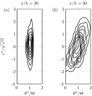
The mixing processes in the inner and outer shear layers were further stud-ied using pdfs. In figure 2.2 joint pdfs of the wall normal fluctuating velocity and the fluctuating scalar concentration are reproduced from Ahlman et al.

(26)

16 2. SIMULATION OF TURBULENT FLOW AND MIXING θ00_/Θ v 00/ p v 00 2 x/h = 30 0 1 2 -3 -2 -1 0 1 2 3 (a) θ00_/Θ x/h = 30 0 1 2 -3 -2 -1 0 1 2 3 (b)

Figure 2.2. Joint pdfs of the wall-normal velocity fluctua-tion, scaled by the local rms-value, and the scalar fluctuafluctua-tion, scaled by the local mean. Pdfs acquired at wall normal dis-tances of u00_(y

in) = u00inner peak (a) and yout/yθ_1/2= 1 (b)

(2005). The velocity fluctuation is normalized by the local root-mean-square (rms) of the fluctuation while the scalar fluctuation is normalized by the local mean scalar concentration. Both pdfs shown are extracted from the DNS at a downstream distance of x/h = 30, where the wall-jet is fully turbulent, but at different distances from the wall. The inner pdf is obtained from the position of maximum streamwise fluctuation, and the outer is obtained at the velocity half-width position. The pdfs at the inner and outer location reveal a signif-icant difference in the respective regions. The inner pdf is aligned with the vertical direction, hence indicating that the velocity and scalar fluctuations are uncorrelated. The outer pdf on the other hand exhibits a positive inclination, indicating that low concentration fluid is correlated to velocity fluctuations towards the wall and vice versa.

The turbulence transition region of the simulation was found to occupy a substantial part of the computational domain in the simulations. The applied inlet disturbances consisted of correlated inlet disturbances (Klein et al. 2003). The disturbance length scale was however short, l ¿ h, which most likely reduced the effect of the disturbances on the transition. In the next simulation, an effort was therefore made to improve the inlet disturbances.

(27)

2.3. SUMMARY OF RESULTS IN PAPER 1 17

2.3. Summary of results in paper 1

The simulation in paper 1 concerns a plane wall-jet of the same inlet Reynolds and Mach number as in previous simulations, Re = 2000, M = 0.5. The com-putational domain was increased to 47h × 18h × 9.6h, and the resolution to 384 × 192 × 128 nodes in the streamwise, wall-normal and spanwise directions, respectively. The larger computational domain allowed a more thorough study of the self-similarity of the wall-jet and comparison with the experimental data of Eriksson et al. (1998). Inlet disturbances were generated through a super-position of filtered correlated disturbances, using a length scale of l = h/3, streamwise vortices positioned in the upper shear layer and a periodic forcing in the streamwise component. To reduce negative concentrations in the outer layer, the grid was refined to contain more nodes in the transition region and a second order filter was applied to the scalar over the transition region. The Schmidt and Prandtl numbers of the jet were Sc = 1 and P r = 0.72. Statis-tics of the flow field and the scalar mixing were sampled over a time period of tsamp= 309tj where tj = h/Uinis the inlet time scale of the jet.

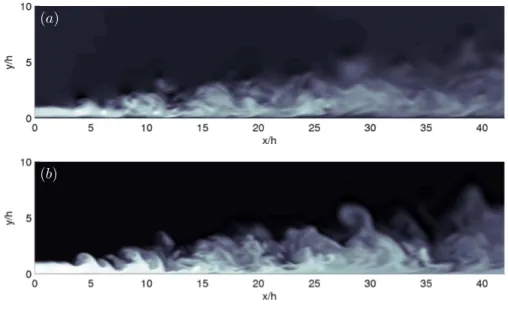
A view of the simulated wall-jet is shown in figure 2.3, where instantaneous solutions of the streamwise velocity and the scalar concentration are plotted in an xy-plane. The jet enter the domain at the lower left corner, and it is seen that the inlet disturbances enforce a quick transition.

(a)

(b)

Figure 2.3. Instantaneous plots of the streamwise velocity, u (a) and the scalar concentration θ (b) in an xy-plane. For the velocity light areas represent positive values and dark negative, while for the scalar light areas represent finite concentration and dark areas correspond to zero concentration.

(28)

18 2. SIMULATION OF TURBULENT FLOW AND MIXING

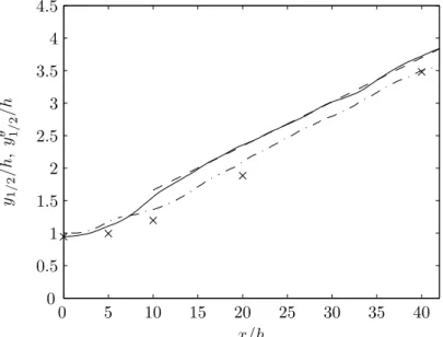
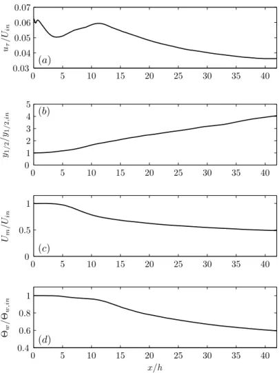
Concerning the spreading rate of the wall-jet, the velocity half-width in-creases approximately linearly with downstream distance, dy1/2/dx = 0.068.

The velocity and scalar half-width exhibit an approximately equal growth rate, which is in contrast to the mixing situation in a plane jet, where the mean scalar profile is wider than the velocity profile. The growth rates obtained from the DNS and the measurements of Eriksson et al. (1998) are shown in figure 2.4.

x/h y1/ 2 /h , y θ 1/ 2 /h 0 5 10 15 20 25 30 35 40 0 0.5 1 1.5 2 2.5 3 3.5 4 4.5

Figure 2.4. Wall-jet growth rate; velocity half-width y1/2/h

(solid), linear fit (dashed), scalar half-width yθ

1/2(dash-dotted)

and experimental values for the velocity half-width by Eriksson et al. (1998) (×).

The maximum streamwise velocity decay, in terms of (Uin− Uc)2/(Um−

Uc)2, is also approximately linear downstream of x/h = 15, whereas in the

ex-periments of Eriksson et al. (1998) the linear behavior is observed at x/h > 70. This difference is presumably owing to the strong disturbances applied in the simulations as well as the difference in Reynolds number.

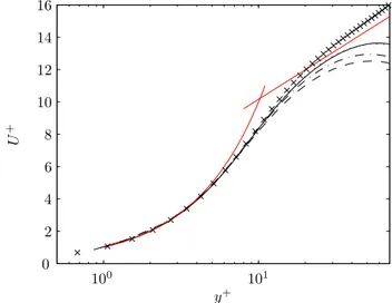
The properties of the inner and outer shear layers were investigated by applying respective inner and outer scaling. In figure 2.5 the mean streamwise profiles are shown in inner scaling, using the friction velocity uτ =

p

τw/ρ and

the corresponding inner length scale l∗ _{= ν/ν}

τ, in accordance with classical

boundary layer scaling. Using inner scaling the mean velocities profiles collapse in the inner region 0 6 y+ ₆_{13. Profiles of the fluctuation intensities were}

also found to collapse in this region using the same inner scaling. A viscous sublayer is found in the profiles, extending out to y+_{= 5, and the position of}

(29)

2.3. SUMMARY OF RESULTS IN PAPER 1 19 layers. The near wall region in a plane-wall jet is thus concluded to resemble a turbulent zero pressure gradient boundary layer. The outer part of the mean

y+ U + 100 ₁₀1 0 2 4 6 8 10 12 14 16

Figure 2.5. Mean velocity profiles in inner scaling (U+_{= U/u}

τ, y+= yuτ/ν) at different downstream positions;

x/h = 15 (dashed), x/h = 20 (dashed-dotted), x/h = 30 (dotted) and x/h = 40 (solid). The linear vis-cous relation U+_{= y}+_{, the logarithmic inertial relation}

U+= _0.381 ln(y+) + 4.1 and DNS data (Reδ∗ = 200) from Skote et al. (2002) (×) are also shown.

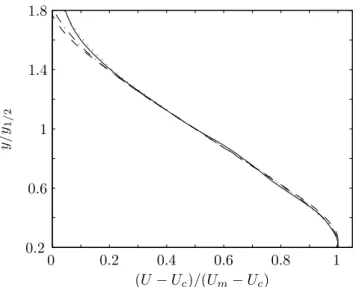
streamwise profiles, from the maximum position and further out, are shown in figure 2.6 using an outer scaling. The velocity difference (Um− Uc) and the

half-width y1/2 are employed for outer scaling, in analogy with what is used

in self-similar plane jets. The outer scaling is found to lead to a collapse of the outer part of the profiles, and hence this region is found to resemble a free plane jet.

The scalar fluctuation intensity is constant in the viscous sublayer in the DNS. In the outer layer the values of the scalar fluctuation intensities corre-sponds to what is observed in a plane jet.

The scaling of the streamwise and wall-normal turbulent scalar flux was also studied. In the outer part of the jet, the flux components are of comparable magnitudes, although the mean scalar gradient is approximately perpendicu-lar to the wall. In the inner region the streamwise flux intensity increases with downstream distance, attaining significant values at x/h > 30. Non-zero streamwise flux has previously been observed in channel flow and in plane jets, and can be explained by observing that the production term of the scalar flux transport equation is non-zero.

(30)

(U − Uc)/(Um− Uc) y /y 1 / 2 0 0.2 0.4 0.6 0.8 1 0.2 0.6 1 1.4 1.8

Figure 2.6. Mean velocity profiles in the outer shear layer, using an outer scaling adjusted for the coflow. Profiles at in-creasing downstream positions; x/h = 15 (dashed), x/h = 20 (dashed-dotted), x/h = 30 (dotted) and x/h = 40 (solid)

(31)

Acknowledgements

I would first and foremost like to express my gratitude to my supervisors, for their invaluable guidance and support. Professor Arne Johansson; your vast knowledge in fluid mechanics, in combination with your management skills, are ever encouraging. Doctor Geert Brethouwer; thank you for introducing me to direct numerical simulations, and for taking the time to answer all my questions on it.

The Centre for Combustion Science and Technology (CECOST) and the Swedish Energy Agency (Energimyndigheten) are gratefully acknowledged for financing this work.

Computer time have been provided by The Swedish National Allocation Committee (SNAC). The simulations were carried out using resources at The Center for Parallel Computers (PDC) at The Royal Institute of Technology (KTH).

A special thanks is extended to Doctor Bendiks Jan Boersma, for providing the original version of the simulation code, and for extensively answering my questions on numerical techniques.

I would like to thank Docent Tony Burden for examining and providing valuable feedback on the combustion background. I am also indebted to Doctor Gunnar Tibert for scrutinizing the thesis, and for fatherly guiding me in the art of scientific typesetting. Anders Ros´en is acknowledged for discussions on any and all aspects of computers, at just about any time of the day.

All colleagues at the Department of Mechanics are thanked for providing a friendly and inspiring environment. In particular I would like to thank the past and present inhabitants of Plan 8, for always bringing a smile to my face. The lunch gang are greatfully acknowledged for providing me with numerous oppor-tunities for uncontrollable laughter. All great friends outside of the Department are thanked for being precisely that.

Slutligen vill jag tacka min familj för all kärlek, stöd och uppmuntran!

(32)

Bibliography

Ahlman, D., Brethouwer, G. & Johansson, A. V.2004 Simulation and mixing in a plane compressible wall jet. In Advances in Turbulence X , pp. 369–372. Ahlman, D., Brethouwer, G. & Johansson, A. V.2005 Direct numerical

sim-ulation in a plane compressible and turbulent wall jet. In Fourth international symposium on Turbulence and Shear Flow Phenomena, pp. 1131–1136.

Ahlman, D., Brethouwer, G. & Johansson, A. V.2006 A numerical method for simulation of turbulence and mixing in a compressible wall-jet. Tech. Rep. Dept. of Mechanics, Royal Instutute of Technology.

Bilger, R. W.2000 Future progress in turbulent combustion research. Prog. Energy Combust. Sci. 26, 367–380.

Boersma, B. J. 2004 Numerical simulation of the noise generated by a low Mach number, low Reynolds number jet. Fluid Dyn. Res. 35 (6), 425–447.

Bruneaux, G., Akselvoll, K., Poinsot, T. & Ferziger, J. H.1996 Flame-wall interaction simulation in a turbulent channel flow. Combust. Flame 107, 27–44. Bruneaux, G., Poinsot, T. & H., F. J.1997 Premixed flame-wall interaction in a turbulent channel flow: budget for the flame surface density evolution equation and modeling. J. Fluid Mech. 349, 191–219.

Conaire, M. O., Curran, H. J., Simmie, J. M., Pitz, W. J. & Westbrook, C. K. 2004 A comprehensive modeling study of hydrogen oxidation. Int. J. Chem. Kinet. 36, 603–622.

Curran, H. J., Gaffuri, P., Pitz, W. J. & Westbrook, C.2002 A comprehensive modeling study of iso-octane oxidation. Combust. Flame 129, 253–280. Dabrieau, F., Cuenot, B., Vermorel, O. & Poinsot, T. 2003 Interaction of

flames of H2+ O2with inert walls. Combust. Flame 135, 123–133.

Eriksson, J. G., Karlsson, R. I. & Persson, J.1998 An experimental study of a two-dimensional plane turbulent wall jet. Experiments in Fluids 25, 50–60. Klein, M., Sadiki, A. & Janicka, J. 2003 A digital filter based generation of

inflow data for spatially developing direct numerical or large eddy simulations. J. Comp. Phys. 186, 652–665.

Klimenko, A. Y. & Bilger, R. W.1999 Conditional moment closure for turbulent combustion. Prog. Energy Combust. Sci. 25, 595–687.

Launder, B. E. & Rodi, W. 1983 The turbulent wall jet – measurements and modelling. Ann. Rev. Fluid Mech. 15, 429–459.

(33)

Levin, O., Chernoray, V. G., L¨ofdahl, L. & Henningson, D.2005 A study of the blasius wall jet. J. Fluid Mech. 539, 313–347.

Peters, N.1971 Laminar flamelet concepts in turbulent combustion. In Twenty-First Symposium (Int.) on Combustion, pp. 1231–1250. The Combustion Institute, Pittsburgh.

Peters, N.2000 Turbulent Combustion. Cambridge University Press.

Pitsch, H.2006 Large-eddy simulation of turbulent combustion. Ann. Rev. Fluid Mech. 38, 453–482.

Poinsot, T., Candel, S. & A., T.1996 Applications of direct numerical simulation to premixed turbulent flames. Prog. Energy Combust. Sci. 21, 531–576. Poinsot, T., Haworth, D. C. & G., B.1993 Direct simulation and modeling of

flame-wall interaction for premixed turbulent combustion. Combust. Flame 95, 118–132.

Poinsot, T. & Veynante, D.2001 Theoretical and Numerical Combustion. R.T. Edwards.

Pope, S. B.1985 Pdf methods for turbulent reactive flows. Prog. Energy Combust. Sci. 11, 119–192.

Pope, S. B.2000 Turbulent Flows. Cambridge University Press.

Skote, M., Haritonidis, J. H. & Henningson, D.2002 Varicose instabilities in turbulent boundary layers. Phys. Fluids 14 (7), 2309–2323.

Spalding, D.1971 Mixing and chemical reaction in steady confined turbulent flames. In Thirteenth Symposium (Int.) on Combustion, pp. 649–657. The Combustion Institute, Pittsburgh.

Stanley, S. A., Sarkar, S. & Mellado, J. P.2002 A study of flow-field evolution and mixing of in a planar turbulent jet using direct numerical simulation. J. Fluid Mech. 450, 377–407.

Vervisch, L. & Poinsot, T. 1998 Direct numerical simulation of non-premixed turbulent flames. Ann. Rev. Fluid Mech. 30, 655–691.

Veynante, D. & Vervisch, L.2002 Turbulent combustion modeling. Prog. Energy Combust. Sci. 28, 193–266.

Wang, Y. & Trouv´e2005 Direct numerical simulation of nonpremixed flame-wall interactions. Combust. Flame 144, 461–475.

Wikstr¨om, P. M., Wallin, S. & Johansson, A. V.2000 Derivation and investi-gation of a new explicit algebraic model for the passive scalar flux. Phys. Fluids 12_{, 688–702.}

(34)

(35)

Part II

Papers

(36)

(37)

Paper 1

(38)

(39)

Direct numerical simulation of a plane

turbulent wall-jet including scalar mixing

By Daniel Ahlman, Geert Brethouwer and Arne V.

Johansson

KTH Mechanics, SE-100 44 Stockholm, Sweden To be submitted

Direct numerical simulation is used to study a turbulent plane wall-jet including the mixing of a passive scalar. The inlet based Reynolds and Mach numbers are Re = 2000 and M = 0.5 respectively. A constant coflow of 10% of the inlet jet velocity is applied above the wall-jet. The passive scalar is added to the jet, at the inlet, in a non-premixed manner, enabling the investigation of the wall-jet mixing as well as the dynamics. The mean development and the respective self-similarity of the inner and outer shear layers are studied. Comparisons of properties in the shear layers of different character are performed by applying inner and outer scaling. The characteristics of the wall-jet is compared to what is reported for other canonical shear flows. In the inner part, out to approximately y+_{= 13, the wall-jet is found to closely resemble a zero pressure}

gradient boundary layer. The outer layer is found to resemble a free plane jet. The downstream growth rate of the scalar is approximately equal to that of the streamwise velocity, in terms of the growth rate of the half-width. The scalar fluxes in the streamwise and wall-normal direction are found to be of comparable magnitude.

1. Introduction

A plane wall jet is obtained by injecting fluid, with high velocity parallel to a wall, in such a way that the velocity of the fluid over some distance from the wall supersedes that of the ambient flow. The structure of a turbulent wall jet can be described as composed of two canonical shear layers of different character. The inner shear layer, from the wall to the point of maximum streamwise velocity, resembles a boundary layer, while the outer layer from the maximum velocity out to the ambient fluid resembles a free shear layer. A consequence of the double shear layer structure is that properties such as momentum transfer and mixing will exhibit distinctively different character and scalings in the two shear layers.

Plane wall jets are used in a wide range of engineering applications. Many of these applications apply wall jets to modify heat and mass transfer close

(40)

30 Daniel Ahlman, Geert Brethouwer and Arne V. Johansson

to walls. Well known examples of these are e.g. film-cooling of leading edges of turbine blades and in automobile demisters. In the first applications, the purpose is to use a cool layer of fluid to protect the solid surface from the hot external stream, while in the case of the demister, warm jet fluid is used to heat the inside of the wind shield. An important aspect in these applications is turbulent mixing in the vicinity of walls. However, the mixing processes in this region are presently not fully understood, and it is therefore of interest to add to this knowledge. An extended understanding of the mixing properties close to walls is also of relevance for applications containing combustion. In most combustion systems, such as in internal combustion engines and in gas turbines, part of the combustion takes place in the vicinity of walls. The aim of the present simulation effort is hence to study the dynamics and mixing in a plane wall jet.

The first experimental work on plane wall jets was carried out by F¨orth-mann (1936). He concluded that the mean velocity field develops in a self-similar manner, the half-width grows linearly and that the maximum velocity is inversely proportional to the square root of the downstream distance. Glauert (1956) studied the wall jet theoretically, seeking a similarity solution to the mean flow by applying an empirical eddy viscosity model. However, because different eddy viscosities are needed in the inner and outer part of the jet he concluded that a single similarity solution is not possible. Bradshaw & Gee (1960) were the first to present turbulence measurements from a wall-jet and reported that the shear stress attains a finite value at the point of maximum velocity. Tailland & Mathieu (1967) reported a Reynolds number dependency of the half-width growth and maximum velocity decay.

The wall jet experiments carried out prior to 1980 have meritoriously been compiled and critically reviewed by Launder & Rodi (1981,1983), using the fulfilment of the momentum integral equation as a criterion to asses the two-dimensionality of the experiments. In the experiments considered to be satis-factorily two-dimensional, the linear spreading rates were found to fall within the range dy1/2/dx = 0.073 ± 0.002. The position of zero shear stress was

concluded to be displaced from the position of maximum velocity, however the uncertainties in the turbulence statistics were reported to be high. In the exper-iments reviewed no near-wall peak in the energy was found. This was assumed to result from the strong influence of the free shear layer on the inner layer. In the study of Abrahamsson, Johansson & L¨ofdahl (1994), inner maxima were found in the experimental streamwise and lateral turbulence intensities, however the calculated kinetic energy did not possess an inner peak, only a tendency towards a plateau.

Schneider & Goldstein (1994) used LDV to measure turbulence statistics in a wall-jet at Re = 14000. They found the Reynolds stresses in the outer region to be higher than the previous data acquired using hot-wire measurements, which underestimated properties in this region. LDV was also used by Eriksson, Karlsson & Persson (1998), to perform highly resolved velocity measurements

(41)

DNS of a plane turbulent wall-jet including scalar mixing 31 in a wall jet of Re = 9600 all the way into the viscous sublayer, enabling direct determination of the wall shear stress. In accordance with other flows, scaling laws for the velocity and Reynolds stress profiles, have been sought for the plane wall jet. One first choice is to make use of the velocity and jet height at the inlet as the characteristic scales, but this does not lead to a collapse the data from different experiment in an convincing manner (see e.g. Launder & Rodi 1981). Using a different approach, Narashima, Narayan & Parthasarathy (1973) suggested that the mean flow parameters should scale with the jet momentum flux and the kinematic viscosity. The same approach was employed by Wygnanski, Katz & Horev (1992) in an effort to remove the inlet Reynolds number dependency and to determine the skin friction from the decrease in momentum flux. Wygnanski et al. (1992) also reported that the assumption of constant Reynolds stress in the overlap region does not hold for a wall jet. Irwin (1973) used a momentum balance approach, neglecting viscous stresses, to derive that in the case of jets a coflow, the ratio of the streamwise velocity to the coflow must be kept constant for strict self-similarity to be possible. Also for the wall jet in an external stream Zhou & Wygnanski (1993) proposed a scaling based on the work of of Narashima et al. (1973).

Concerning the wall jet in quiescent surroundings, George et al. (2000) performed a similarity analysis of the inner and outer part of the wall jet. Both the inner and outer region were reported to reduce to similarity solutions of the boundary layer equations in the limit of infinite Reynolds number, however for finite Reynolds numbers, neither inner nor outer scaling leads to a complete collapse of the data.

The task of computing solutions to the plane wall jet has proven to be challenging. Part of the problem arises from the combination of two distinct shear layers in the wall jet. Since the two regions interact strongly, many char-acteristics of wall jets differ from those of other canonical shear layers. Early computational efforts using RANS type methods are reviewed by Launder & Rodi (1983), more recent attempts are reviewed by Gerodimos & So (1997). Tangemann & Gretler (2001) proposed an algebraic stress model and compared it to the standard k–² model and a full Reynolds stress model by computing a two-dimensional wall jet in an external stream. They found the algebraic and the Reynolds stress model, but not the k − ² model, to be able to produce a region of negative production of turbulent kinetic energy where the inner and outer shear layers interact. Dejoan & Leschziner (2005) performed a highly resolved large eddy simulation (LES) matching the experiments by Eriksson et al. (1998). The simulation was found to agree well with the experiments, also for the Reynolds stresses. By examining the budgets of the turbulent energy and Reynolds stresses, the turbulent transport was found to play a par-ticularly important role in the region where the outer and inner layers overlap. The transition process was reported difficult to accurately reproduce in LES, and a defect in the wall-normal stress in the simulation was attributed to this difficulty.

(42)

Reports of direct numerical simulations (DNS) of wall jets, have up to recently been scarce, even more so for investigations providing time averaged statistics. Wernz & Fasel (1996,1997) employed DNS to investigate the impor-tance of three-dimensional effects in the transition of wall jets. The breakdown of a finite-aspect-ratio wall jet was studied by Visbal, Gaitonde & Gogineni (1998). Recently Levin et al. (2005) studied a wall jet both experimentally and by means of DNS. In the simulation two-dimensional waves and optimal streaks corresponding to the most unstable scales were introduced in a wall jet at Re = 3090. The presence of streaks were found to suppress pairing and to enhance the breakdown to turbulence. In an extension to the previous work, Levin (2005) used the same forcing and a larger computational box to obtain turbulence statistics.

Despite the numerous investigations of wall jets, including theoretical, ex-perimental simulation studies, the question of self-similarity and proper scaling is not fully understood. The reason for this originates in the existence of two different types of shear layers. Each of the layers have a distinct set of charac-teristics and scalings which excludes a full self-similarity of the wall jet. Pre-sumably statistics close to the wall are governed by inner scales, in accordance to boundary layers, and likewise in the outer part, where some type of outer scales will be the appropriate ones. However, the definition of scalings is not clear, and may as well vary between different quantities.

The aim of the present investigation is to study the turbulent propagation of a plane wall-jet by means of direct numerical simulation. The study aims at increasing the knowledge of the dynamics and mixing present in this flow case. Presently, few simulations have been performed for this flow case, and this is to the authors’ knowledge the first to include scalar mixing.

In the simulation an effort is made to provide efficient inlet disturbances in order to facilitate a fast and efficient transition to turbulence. The research is part of an ongoing project with the aim of studying turbulent combustion through DNS. Since realistic simulations of combustion involve heat release and considerable density fluctuations, the fully compressible formulation of the fluid dynamics problem is used.

In terms of dynamics characteristics, both mean development and fluctua-tions of the wall-jet are of interest. The mean development is characterized by investigating the jet spread rate and the decay of the streamwise velocity. The different properties of the inner and outer layers are investigated by applying different scalings in the respective layers. It is of interest to determine the different dynamical properties of these layers and to relate them to what has previously been found for other canonical shear flows, such as e.g. boundary layers and free shear flows. The different scaling approaches are also valuable in assessing to what extent the wall-jet can be considered self-similar. In terms of mixing, the wall jet provides an interesting flow case with implications for engineering applications, since it involves mixing in the vicinity of a wall. Mix-ing in this region is of importance for example in development and investigation

(43)

DNS of a plane turbulent wall-jet including scalar mixing 33 of combustion models for accurate predictions in the presence of a wall. For this reason scalar properties in the wall-jet in the inner and outer region of the wall-jet, such as scalings and self-similarity, is studied in analogy to those of the velocity field.

2. Governing equations

The equations governing conservation of mass, momentum and energy (see e.g. Poinsot & Veynante 2001) are

∂ρ ∂t + ∂ρuj ∂xj = 0, (1) ∂ρui ∂t + ∂ρuiuj ∂xj = − ∂p ∂xi +∂τij ∂xj , (2) ∂ρE ∂t + ∂ρEuj ∂xj = − ∂qj ∂xj +∂(ui(τij− pδij) ∂xj , (3)

where ρ is the mass density of the fluid, ui the velocity components, p is the

pressure and E = (e + 1/2uiui) is the total energy. The fluid is considered

to be Newtonian with a zero bulk viscosity, for which the general form of the viscous stress is τij= − 2 3µ ∂uk ∂xkδij+ µ µ_∂u i ∂xj + ∂uj ∂xi ¶ , (4)

where µ is the dynamic viscosity. The heat diffusion is approximated using Fourier’s law for the heat fluxes qi = −λ∂T/∂xi where λ is the coefficient of

thermal conductivity and T is the temperature. In the simulations a Prandtl number of

P r = ν λ/(ρCp)

= 0.72, (5)

is used. The fluid is furthermore assumed to be calorically perfect and to obey the perfect gas law. The compressibility of the jet is parameterized by the Mach number. To keep the compressibility effects small, while maintaining reasonably large simulation time steps, a moderate Mach number is used. The inlet Mach number of the simulation is set to M = Uin/a = 0.5, where Uin is

the velocity at the inlet and a is the speed of sound.

The mixing in the plane wall jet is studied by introducing a passive scalar in the simulations. The scalar is conserved i.e. no production or destruction of the scalar is present and the scalar is passive in the sense that the motion of the fluid is unaffected by the presence of the scalar. The equation governing the passive scalar concentration, θ, is (see e.g. Poinsot & Veynante 2001),

∂ρθ ∂t + ∂ ∂xj (ρujθ) = ∂ ∂xj µ ρD ∂θ ∂xj ¶ (6) where D is the diffusion coefficient of the scalar. In the simulations the scalar diffusivity in terms of the Schmidt number is Sc = ν/D = 1.

(44)

3. Numerical method

3.1. Spatial integration

Spatial integration of the governing equations is achieved by employing a for-mally sixth order compact finite difference scheme for the first derivative (Lele 1992). In the non-periodic directions, schemes of reduced order are used at the nodes close to the boundary. At the node directly on the boundary, a one-sided third order scheme is used. At the consecutive node a central fourth order scheme is used.

3.2. Temporal integration

For the temporal integration an explicit Runge-Kutta scheme of third order is employed. The scheme is four stage, formulated in low-storage form and is presented in Lundbladh et al. (1999). During simulation the linear CFL number is kept constant, varying the time step.

3.3. Computational domain

The computational domain used in the simulations consists of a rectangular box. The physical domain size, in terms of the jet inlet height h, is Lx/h =

47, Ly/h = 18 and Lz/h = 9.6 in the streamwise, wall-normal and spanwise

directions respectively. The inlet of the jet is positioned directly at the wall with the flow parallel to it. In the simulation, the streamwise and the wall-normal directions are non-periodic, while the spanwise direction is treated periodically.

3.4. Grid stretching

The computational domain is discretized using a structured grid. The number of nodes used in the simulation is 384 × 192 × 128, in the streamwise, wall-normal and spanwise direction respectively, amounting to a total of 9.4 × 106

nodes. The grid employed is stretched in the wall-normal and the streamwise direction but uniform in the spanwise.

In the streamwise direction a third order polynomial is used to stretch the grid. The grid spacing is finest in the transition region of the jet, and coarsest at the outlet, maintaining a node separation of 10 < ∆x+_{< 12 in terms of wall}

units in the developed region used for turbulent statistics 15 6 x/h 6 40. Also in wall units, the spanwise node separation decreases from ∆z+(x/h = 15) = 8.2 to ∆z+_{(x/h = 40) = 5.5 in the developed region.}

In the wall-normal direction, the grid is stretched using a combination of a hyperbolic tangent and a logarithmic function. The combination allows for clustering of nodes close to the wall while maintaining a high resolution of the outer layer. In the inner region, the viscous sublayer, y+ _{< 5, is always}

resolved with three or more nodes. In the outer layer the wall-normal node spacing equals that of the spanwise direction at a wall distance y = 2.9h.