of the inflation rate?
and can it be improved?
Author:
Serdar Akin
Master’s Thesis
Economics
couraging guidance, insightful comments, support during the writing of this thesis and helping me into exploring reproducible econometrics.
Abstract
The focus of this paper is to evaluate if forecast produced by the Central Bank of Sweden (Riksbanken) for the 12 month change in the consumer price index is unbiased? Results shows that for shorter horizons (h < 12) the mean forecast error is unbiased but for longer horizons its negatively bi-ased when inference is done by Maximum entropy bootstrap technique. Can the unbiasedness be improved by strict ap-pliance to econometric methodology? Forecasting with a linear univariate model (seasonal ARIMA) and a multivari-ate model Vector Error Correction model (VECM) shows that when controlling for the presence of structural breaks VECM outperforms both prediction produced Riksbanken and ARIMA. However Riksbanken had the best precision in their forecast, estimated as MSFE.
Keywords: Inflation rate, VECM, Structural Breaks, Rolling-event forecast, Maximum Entropy bootstrap, ARIMA
1 Introduction 1
2 Forecasting 3
2.1 Data. . . 3
2.2 Strategy . . . 4
3 Forecast evaluation for Riksbanken 7 4 Econometric Model building 7 4.1 Structural Breaks . . . 8
4.2 Variable Selection . . . 10
4.3 Forecast evaluation for ARIMA. . . 11
4.4 Forecast evaluation for VECM . . . 12
5 Comparing the forecasts 13 6 Discussion 13 Appendix A: Graphs 17 Appendix B: Tables 21
List of Figures
1 Descriptive statistic. . . 172 Mean Forecast Error (MFE) for Riksbanken (RB) . . . 18
3 MFE for ARIMA and VECM . . . 19
1
Introduction
The cause and consequence of hyper-inflation created the need for an independent central bank that was legally committed to refuse the governments demand for unsecured credit. The aftermath of world war one showed why price stability is desirable. Price stability facilitates the role of the payment system, reduces uncertainty in firms and households investment decision and prevents arbitrary redistribution of income and wealth (Berg,2000, 4). In 1931, Sweden became the first country to make stabilization of the domestic price level the official goal of its monetary policy (Berg,2000). In November 1992 Sweden were forced to abandon the fixed exchange rate and conduct policy aiming at inflation targeting. The objective is to keep the inflation rate at 2± 1 per cent measured as the yearly change in the consumer price index. Nowadays the tolerance band is removed (Assarsson, 2010, 47). In an effort to make the Riksbanken more effective in monetary stability as well as stabilizing the real economy a number of legislative changes came into force at January 1999 that made the Riksbanken more independent. The institutional framework for Riksbanken rest on three pillars (Svensson,2009, 1),
(1) A mandate for monetary policy from the government or parliament, normally to maintain price stability.
(2) Independence for the central bank to conduct monetary policy and fulfill the mandate.
(3) Accountability of the central bank for its policy and decisions.
The second pillar means that there is no appliance for Riksbanken to tie it self into a strict inflation targeting. Flexible inflation targeting means that monetary policy aims at both stabilizing the inflation around the inflation target and to stabilize the real economy. The importants of this trade-off is best understood by considering a negative supply shock that both raises prices and decreases output. If Riksbanken, in an effort to apply strict inflation targeting, would raise the repo rate without considering the effect it has on the real economy, a likely cause would be that the unemployment rate would increase further. Since investment is negatively correlated with the real interest rate a rise in the repo rate during this stage would further dampen output and causing the recession to become more severe (Svensson, 2009, 2). Later years Riksbankens responsibility has increased by aiming at stabilizing asset prices e.g., real estate prices. Riksbanken has to prevent asset price bubbles to burst since this affects real-economic variables and the inflation rate negatively (Assarsson, 2010, 48). Policy instrument at Riksbankens disposal is the repo rate which due to transmission mechanism is set by judgemental forecasting procedure. Forecasting procedure for the Riksbanken is first to estimate
a future path of e.g., the inflation rate, using econometric models like the so-called “RAMSES”1, which incorporates open economy aspects and Bayesian VAR2, where
non-sample information can be used (Hallsten and T¨agtstr¨om, 2001, 73). The reported forecast in the inflation report is the product of judgments made by the executive board, which based on their analytical ability as well as experience make the necessary changes that they perceive to best reflect the economic condition at the time as wells as prediction produced by econometric models (Hallsten and T¨agtstr¨om, 2001, 72).
The last pillar, accountability, makes Riksbankens monetary policy important to analyze. Since Riksbanken cannot control the inflation rate perfectly and that it lacks perfect knowledge of the way their policy are going to affect the economy their is going be deviation between outcome and prediction. For a forecast to be optimal a necessary condition is unbiasedness, In a paper for testing whether the Riksbanken systematically over/under predicted the forecast of inflation rate, Lundholm (2010) showed that there is a negative bias in the mean forecast error up to a one years forecast horizon and a positive bias above one year3. This implies that there is a
systematic tendency for the Riksbanken to not produce optimal prediction. This paper focuses on testing whether the Riksbanken:s forecast on the inflation rate still is biased for the time period 1999:M6-2011:M3. Test of unbiasedness is done by regression method called “rolling-event forecast surveys”. Results shows that for forecast horizons less than one year all inference methods are almost significantly unbiased4 but for 12-25 horizons there is a significant negative bias when estimation
are formed from the ME bootstrapping technique.
Those estimation will be the reference point when testing whether econometric models yield better prediction than do Riksbanken. Forecasts are produced by a linear seasonal Autoregressive Integrated Moving Average (ARIMA) model and by a multivariate model Vector Error Correction Model (VECM). Most unbiased horizons were found for when controlling for the presence of Structural Breaks (SB) using the forecast produced by the VECM. In this context, if SB is one factor that causes bias will be analyzed.
This paper unfolds in the following way. Section2describes the dataset collected from Riksbanken and changes that has happened during the sample period, followed by theoretical discussion on rolling-event forecast surveys. In section3the empirical
1 Riksbankens Aggregerade Makromodell f¨or Studier av Ekonomin i Sverige
2 Research in the area has shown that for short term horizons econometric models like Vector
autoregression (VAR) does a very good job at forecasting the inflation rate (IR)Riksbanken (Inflation report 2006, p.57)
3 Lundholm(2010) uses Maximum Entropy (ME) bootstrapping for this to hold and between
time period 1999-2007
4 Results are estimated by Ordinary Least Square (OLS), Heteroskedasticity and Autocorrelation
results from the forecast evaluation of Riksbanken using the method of rolling-event forecast are presented. Section 4 discusses econometrics models and the selection process for the VECM. This sections concludes with empirical results produced from the econometric models. Section (5) estimates the precision estimated as MSFE and compares the forecast for all three forecasters. The final section concludes. Graphs and tables that underpins this paper are presented in the appendix, A further digest of econometric theory is shown in the accompanied technical documentation.
2
Forecasting
2.1
Data
Inflation is defined as a “a rise in the general level of prices of goods and services in an economy over a period of time”. The first aim is to collect a dataset that is comparable during the time-period of interest. The inflation rate is the 12 month change updated monthly from the consumer price index. In an effort to have a high degree of transparency Riksbanken publishes inflation reports that consist of forecast of e.g., the repo rate, inflation rate and other different sorts of statistics. Those reports are the source from where each vector of prediction that the Riksbanken produce are collected from. The total number of inflation reports that are published between 1999:Q2-2009:Q1 is 39, henceforth will be called target dates. Between 1999-2005 inflation reports were reported four times a year5 and
afterward it were reduced to three reports a year. Linear interpolation is done for the last quarter in 2006 and follow-up reports are used for the last quarter between years 2007-2008. This gives a total of 40 target dates.
The choice of target horizon is very contingent on the lag with which monetary policy affects inflation rate6 and experience in Sweden has suggested that the lag
before policy elicits its main effect is 1-2 years (Berg, 2000, 15). In an effort to show to the public how the development of inflation is affected by temporary effects Riksbanken increased there forecast horizon from year 2006 onwards to 36 months
Riksbanken (Inflation report 2005, p.50). In this paper the forecast horizon will be 25 months throughout each target dates. Hence the final dataset will be a (25 × 40)
matrix. This makes it necessary to have data until 2011:M3 since pseudo out of sample forecasting is done to the final target date at 2009:Q1.
5 Mostly they were published in Mars, June, October and December but can differ sometimes. 6 The so-called transmission mechanism of monetary policy can be divided into two phases, first
how it affects nominal interest rates (Stibor rate is the interest rate that intermediate financial institutions borrow and lend money to each other) which in turn affects the aggregated demand. The second phase is of how the aggregated demand succeeds in affecting the inflation rate. Both phase is considered to take approximately 12 months eachBain and Howells(2009, 123)
Before January 2005 the forecast of inflation rate were based on an assumption of constant repo rate during the reported forecast horizon. In 2005 it were decided that this assumption was not a realistic assumption, so instead the repo rate would move according to implicit forward rate over the forecast horizon Riksbanken
(Inflation report 2005, p.50). Since February 2007, the forecast for inflation rate is based on the Riksbankens best forecast for the future repo rate (Svensson, 2009, 6). As of December 1997, Riksbanken uses forecast with uncertainty intervals, visualized as fan charts for different confidence interval. Those graphs are then used for communicating with the public about their perceived future path of e.g., the inflation rate. Confidence interval are based on historical forecast error.
Figure (1) (page 17) shows the mean and variance for the forecast error (FE), and the repo rate along with its target. FE is defined in equation (2.3). Seemingly there is two areas with negative means and large variation in figure (1a). At the same time the yearly inflation rate were outside its former tolerance band of 2± 1
per cent seen in figure (1b). Sudden increases in the inflation rate are mostly caused by increased energy and/or food prices. For instance at the beginning of 2001 one factor of the sudden price increase in the inflation rate was because of a increase in the food prices brought to about by the mad cow and foot-and-mouth diseases. And in year 2003 the increase in the inflation rate were due to increases in the energy prices. Extremely high electricity prices brought by cold and dry weather caused the inflation rate to increase to high levels and were followed by unusually low inflation rate when electricity prices decline during summer and spring of 2003. The inflation rate were reinforced due to the so-called dotcom crisis and terrorist attack on the US at 9/11. The next larger increase in the inflation rate and negative mean were due to the financial crisis which began late 2007. At 2007-10 for instance, the mean forecast error were -0.8 and dropped to -2.3 at 2008-07. Both crisis gave rise to a negative mean forecast error since Riksbanken over-predicted the future path of the inflation rate. Only at years 2005-2007 did the mean forecast error become very close to equal zero.
For reproducible econometric this paper uses open source program. To keep everything in a single file Docstrip7 is being used, writing is in LATEX mode using
text-editor GNU Emacs 23.2. For statistical programming R2.12is used in ESS 5.12. This study has a accompanied technical document which consist of tables and further detailed exposition of the methods used that underpins this paper. R-codes is shown in “rcode.pdf” which is produce in an effort to make reproducibility more easier.
2.2
Strategy
Inflation bias is caused when (1) governments see votes in higher output and (2) governments see votes in generous public service (Bain and Howells,2009, 235). The problem when the Riksbanken perceives a higher output to be favorable relative to a stable inflation rate can be seen when Riksbanken relaxes their policy instrument and knows the location of the aggregated demand curve, the negative correlation between investment and the real interest rate will cause a shift to the right. Inflation pressure is build up since the economy exceeds the long-term production capacity. This will cause wages to rise. Firms will compensate this by further increasing the prices on their output. Eventually equilibrium is restored but with a higher inflation rate. So Riksbanken can only affect the real economy at the expense of a higher inflation rate. This is sometimes called the Taylor Rule8
Their is lots of conceivable reason for why forecast errors arises. One reason may be due to the assumptions inherent in symmetric versus asymmetric loss function, meaning that there is different cost associated with the gains and losses. Clements and Hendry (2000) mean that if there is asymmetry loss function, so that there are proportionately greater cost attached to, say under-prediction than over-prediction, an optimal predictor would on average over-predict. For example, a trade union bargaining over nominal wages, which intent on obtaining a minimum real wage for its members, may attach greater costs to under-predicting the inflation than being wrong in the other direction (Clements and Hendry, 2000, 34). An optimal predictor for a quadratic loss function given the information set It is as follows,
(2.1) Pt +h|T= argminE
�
(et +h|T)2|It
� ,
where the FOC becomes
E�−2et +h|T�=E�et +h|T�= 0,
(2.2)
Equation (2.2) shows that in order for Pt +t |T to be a optimal predictor unbiasedness
is a necessary condition. Testing for unbiasedness is done with rolling-event forecast surveys which holds the horizon (h) fixed between the target dates. Then the Forecast error (e) at time T for horizon h is calculated as:
(2.3) et +h|T=At +h−Pt +h|T,
where notations are the following. Actual (A) and Predicted (P) at time T for horizon h. Test of unbiasedness will be done with the regression suggested by
8 The rule stipulates that for each one-percent increase in inflation, the central bank should raise
Holden and Peel (1990) (Clements and Hendry, 2000, 57), (2.4) At +h|T−Pt +h|T= τ + �t +h|T,
if E[At +h−Pt +h] = 0 , then τ = 0 which is same as (2.2) hold (MFE= 0). If �t +h|T is
a white noise then At +h|T−Pt +h|T= 0 gives expectation E��t +h|T�= 0 and variance
V��t +h|T�= σ. The null-hypothesis in eq. (2.4) is:
H0:MFE= 0 against H1:MFE�= 0.
(2.5)
Accepting the null-hypothesis means that the Riksbanken has made an unbiased forecast at timetfor horizon h. A positive MFE means that the forecaster has under-predicted the inflation rate, while a negative MFE reflects tendency to over-predict. Due to possible serial correlation inference using the OLS may not be valid. To take this into account inference is made with heteroskedasticity and autocorrelation consistent errors HAC and ME bootstrapping (Lundholm,2010, 2). HAC deals with autocorrelation by suggesting the use of linearly decaying weights where the lag is chosen by automatic bandwidth selection procedure and prewhitening the covariance matrix using a VAR(1), which aims at reducing the bias (Zeileis, 2004, 5-6). The principle of Maximum Entropy states: When one has only partial information about the possible outcomes one should choose the probabilities so as to maximize the uncertainty about the missing information, entropy is a measure of the uncertainty associated with a random variable. The advantage of ME bootstrap is that is does not require stationarity (Vinod and de Lacalle,2009). The ME bootstrap shuffle the data J times with replacement9 from where draws allows for (i) close to to original
values, (ii) outside the closed interval defined by sample minimum and maximum ± sample trimmed mean, (iii) preserves the time structure of the data. Around each observation is then an interval formed bounded by the nearest lower and higher values and it is from this interval the bootstrapped value replacing the original observation is drawn (Lundholm,2010, 5).
When the purpose is to compare forecast models for the different horizons the MSFE is a measure of forecast precision. First note that the MFE and MSFE has the following relation,
MSFE(h) = T−1 T � t =1 e2 t +h|T and MFE(h) = T−1 T � t =1 et +h|T, (2.6)
and the variance for the eh,
9 For this study the number of replicates isJ = 999where confidence interval is formed by the
(2.7) V(eh) = T−1 T � t =1 e2 t +h|T− � T−1 T � t =1 et +h|T �2 =MSFE(h) − (MFE(h))2.
Then from (2.7) its clear that the MSFE is:
(2.8) MSFE(h) =V(eh) + (MFE(h))2.
for each h = 1,...,25. If on the other hand all horizons are unbiased then from (2.8) its clear that MSFE will equal the variance for each horizon.
3
Forecast evaluation for Riksbanken
Table (1) (page 21) shows when we fail to rejected null-hypothesis (H0) and (2.2)
holds. Estimates are presented in column two for all three inference techniques. For OLS and HAC almost all horizons are unbiased. However, considering the ME bootstrap the MFE is equal to zero in the interval for 4 -11. The mean of MFE in column 3-5 shows that most of the negative bias in for horizons more than a year (h≥ 12). Graphs has the advantage of putting a very large number of estimates into a small and delimited space. This gives a better comparability than e.g., a table. In figure (2) (page 18) results derived from all three inference methods is shown. The red horizontal dashed line shows that when its between the confidence interval of the respective method then this horizons is unbiased. ME bootstrap has no confidence interval at horizons between 1-3 which means that there is almost none variation between trimmed mean, or the maximum and minimum value. Its clear that for h≥ 12 estimates with ME bootstrap shows that none of the MFE is equal to zero. The 95% confidence interval for HAC estimates is not so large and is within the range of ±2, which indicates a small variation in the input data.
Conclusion drawn from a above is that Riksbankens forecast for horizons over 12 months has a systematic negative bias when estimation is done using the ME bootstrap. This means that the predication has been larger than the actual outcome over the longer horizon (see eq. 2.3). From (Clements and Hendry, 2000) then, this would suggest that their is a larger cost in under-predicting the inflation rate than being wrong at the other direction. Or it might reflect the inability for the Riksbanken to control the inflation rate for longer periods.
In this study the role of the tolerance interval which the Riksbanken reports as an estimate for uncertainty has lost its role here since this paper only analyzes a vector of predictions. The further away from the forecast origin the larger the e.g., the 90 per cent confidence interval gets.
4
Econometric Model building
In this section the purpose of testing whether strict appliance to econometric methods will produce optimal forecasts when using a quadratic loss function, meaning that cost and gains are viewed symmetric. When estimating a multivariate model a number of variables that has the power to affect the future path of the inflation rate are tested. In a paper covering the importance of variable selection during forecasting procedure of the Turkish inflation rate, the author found that economic variables like the exchange rate is a important determinant (Omer ¨¨ Ozcicek,
2001, 62) since this variable affects the aggregated demand and supply in the Turkish economy. Further, Omer ¨¨ Ozcicek (2001) shows that it’s important to select a small set of variables that are mainly used when forecasting the inflation rate. In general its accepted that a parsimonious model will produce more accurate forecasts.
Another issue is to increase the knowledge of the statistical properties inherent in the variables that presumably are going to be included in the econometric model. The starting point of this quest is to remove all SB that might prevail in the data. Then determine the integrating order of the variables10. When the integrated order
is known and differenced to become a stationary process, test for determine the predictive power between the inflation rate and all other variable will be done.
For the linear univariate model a seasonal ARIMA model is developed using the Box-Jenkins model selection criteria for parsimony and stationary IR. As for the multivariate model, the first consideration will be whether there is any cointegration between the variables. If not a VAR-specification will suffice for modeling and forecasting the inflation rate, else a VECM has to be modeled. For detecting cointegration both a pairwise and rank test according to the Johansen methodology will be done (L¨utkepohl,2004, 151).
4.1
Structural Breaks
Forecasting without taking into account the presence of a SB causes bias and this bias will be shown here in the context of VAR-specification. A future SB will most likely never be known with certainty but controlling for them within the input data at hand does yield a better forecast than ignoring for this fact. Basically SB are not allowed to affect the forecast.
The occurrence of a SB can be caused by e.g., new legislation that affects the economy or by a new definition of the data series (Pfaff, 2008, 107), e.g., in Sweden a new definition of the Unemployment Rate (UR) is that it includes student as job seekers from 2005:M3 and onwards. If a break occurs at only one point in time
10Else the risk for spurious regression will be predominant, consider two variable X∼I(0) and
and last for the remaining period of the sample, the structural shift is modeled by introducing a step dummy variable in the following way,
Dt=
�
1 if t ≥ T
0 if t < T
Testing for the presence of SB in the variables a linear model that consists of a intercept, trend and seasonality parameters will be employed. More specific the following regression model will detect the presence of SB,
(4.1) xt = β0+ β1t + 12 � i =1 βiSi t+ B � b =1 βb 0+ βb 1t + 12 � i =1 βb iSt b Db t + �t,
where Db t, b = 1,...,B are dummy variable dividing data. B is the optimal number
of breaks11. Intercept correction with a step dummy controls for deterministic shift
that may have happened. Results from the linear model is shown at table (7a) (page 26). A common SB is at dates 08-05 and 08-10. The first date is found for in the indexes as Consumer Confidence Indicator (CCI) and Macro index (MA), and the latter for IR, repo rate or UR. Probably both these dates can be derived to the recent financial crisis that started late 2007.
As said in the beginning of this section its important to controlling for any SB that might be in the data. Removing the SB from the intercept, trend and season is the same as if they were controlled for within the estimated model12 and will reduce
the bias and completely remove it, only whenτ13 changes (so thatΥ∗= Υ)(Clements
and Hendry,2000, 198), E�e∗T+1|xT � = (τ∗− τ) + (Υ∗− Υ)xT, (4.2) E[˜eT+1|xT] = (Υ∗− Υ)∆xT. (4.3)
The conditional FE variance is given by: (4.4) V�e∗T+1|xT
�
= Ω and V[˜eT+1|xT] = 2Ω,
Hence the conditional MSFE is:
11Here breaks are set to include breakpoints up to 5, which imply 6 segments
12Forecasting is done recursively, meaning that the data are updated continually for each target
date.
13Not to be mistaken as notation for MFE as done above. In this section τ is the in-sample
M�e∗T+1|xT � = Ω + [(τ∗− τ) + (Υ∗− Υ)xT][(τ∗− τ) + (Υ∗− Υ)xT]� (4.5) M[˜eT+1|xT] = 2Ω + (Υ∗− Υ)∆xT∆x�T(Υ∗− Υ)�. (4.6)
The second term in (4.5) is then the bias.
4.2
Variable Selection
The initial selected variables that are conceivable on affecting the aggregating demand or supply are discussed here. Since any variable that might affect demand or supply might also might help in predicting the future path of the inflation rate. In the below enumerate a short description for why it is selected in the regression are done.
(i) inflation rate: Is the 12 months change in the consumer price index with the base year 1980 and reported by Statistical Sweden.
(ii) Interest rates: Stibor.3M is the 3 month interest rates/cost that the interme-diate banks have to pay when borrowing money from each other (Interbank market). Data is downloaded as monthly averages between time period 1993:M1-2011:M0214. Government bonds is the long-term interest rate (5 year)
and are issued to finance the governments borrowings needs. The basic stance is that a increase in government bonds is done for financing stimulus packages created by the governments. Repo Rate is the rate the Riksbanken uses to control the Interbank market rate.
(iii) Consumer Surveys: The CCI provides a quick qualitative indication of house-hold plans to purchase durable goods and consumer sentiment on the economic situation in Sweden, personal finances, inflation and savings. The survey cov-ers a sample of 1.500 Swedish households which are interviewed each month. Firms may look at the CCI in order to plan their future inventory and other investments. If CCI views are pessimistic then firms may hold their inventory at low levels and delay investments. Two indexes of inflation expectation today and 12 months ahead will also be tested, as wells as micro and macro index. Mikro index shows how household perceive their own economy to be and macro index for the whole swedish economy.
(iv) Gross Domestic Product (GDP): Is downloaded with the base year 2009 and since GDP is only available in frequency of quarters a linear transformation is done in order to change the frequency to monthly observations. Since the first
quarter of the GDP is reported to the market at approximately at late May or June the first quarter is set to 1993:M6.
(v) Unemployment Rate: Is defined asU/(U+E), and with the population between age 16-64. An excess demand will cause firm to hire more human capital. (vi) Import Index: Is a price index consisting of a total index excluding durable
goods like food and tobacco. Base year is 2005. A sudden rise in the in the relative price of some domestic product will cause, depending of how close of a substitute the product is, increase the level of import. Since Sweden has a floating currency, when the RB raises the repo rate the currency will appreciate due to a increase in capital inflow.
(vii) Total Competitiveness Weights: Is a basket of currencies which enables us to compare the Swedish krona. The starting value is at 18 November 1992. By studying the index one can estimate how the krona has change. A high value means that the krona has deprecated against the basket.
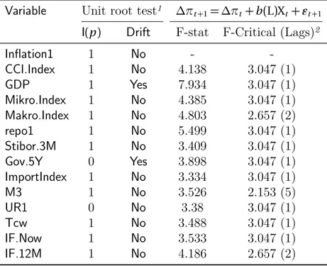
(viii) Money supply: Is the change in the money supply at a given time measured as notes and coins (currency) in circulation outside the RB and other depository institutions. In essence inflation is caused by to much money and to few goods. Table (2) (page22) shows all the test for the above explained variables. Column 2-3 shows the integrating order and drift term for each of the variables. For example the GDP is a random walk with drift. Column 4-5 shows the estimated F-statistic and its critical 5 per cent value estimated by Auto Distributed Lag model. GDP for instance had the largest test statistic. Using those estimates and economic theory the final selection of variables is shown in the first column at table (8) (page 27). The last column is the variables used for predicting the inflation rate were chosen by Granger Causality test15. Table (3b) shows that the Macro index has
a cointegrated relationship between GDP and the Consumer Confidence Indicator. Using the Johansen method the rank test reveals that there is one cointegration vector rank(1)16.
4.3
Forecast evaluation for ARIMA
In this section the procedure for forecasting a linear univariate seasonal ARIMA will be discussed. This model takes account of any seasonal pattern exhibit in the
15See the technical documentation for a further exposition of Granger Causality.
16Since there are 40 target dates the rank test is done recursively. Test shows that 30 out of 40 is
for a Rank (rk)(1) usingλtrace. Forλmax 29 out of 40. Results for rk(2) showed no significance
inflation rate. In addition to the regular AR and MA operators, there are operators in seasonal powers of the lag operator. Such operators can sometimes result in a more parsimonious parameterization of a complex seasonal serial dependence structure than a regular non-seasonal operator (L¨utkepohl,2004, 27).
The aim here is to update the seasonal ARIMA model every time the Riksbanken publishes their inflation report, namely target dates. Since new information enters the input data its possible that the identification process selects another operator than were selected before. The lag operator are decided by the akaike information criterion. For example when controlling for the presence of SB, the first target date were forecasted with the ARIMA(0,1,2)(2,0,0) and for the last target date ARIMA(1,1,0)(1,0,0)17.
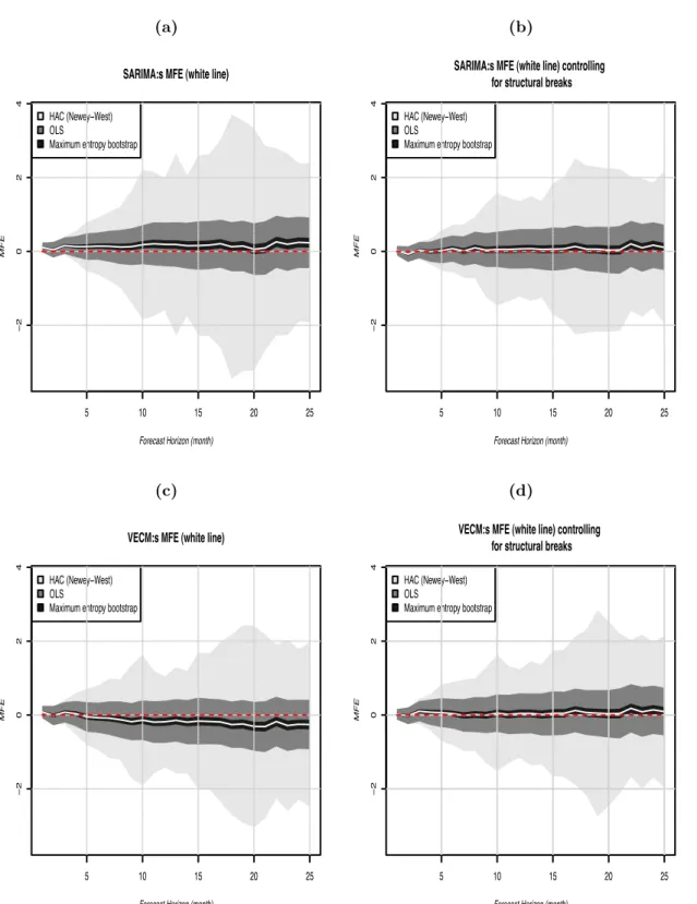
In figure (3a) and (3b) (page 19), the forecast of the ARIMA model is plotted with and without controlling for the presence of SB. In both of the plots all of the estimates are very close to the red dashed line. The interval for HAC corrected standard errors are larger for the model when SB are ignored. When controlling for the presence of SB the variation in the residuals also reduces and this gives a narrower confidence interval. More horizons are also unbiased. In table (4a) (page24) its more clear how improved the models are by controlling for SB. The unbiased estimates in ME bootstrap increases from three to 19. The mean of MFE when controlling for SB shows that most of the positive bias is in the longer horizon. But their is not much difference between the short and long term as for when ignoring the presence for SB. Then ARIMA is positively biased and thus over-predicts the inflation rate. Overall, ARIMA produces unbiased estimates when controlling for SB.
ARIMA models are oftentimes used as a benchmark of whether the researchers own model is better than the pure technical ARIMA model. Hence a researcher should at least ”beat” the ARIMA model for there own model to make sense. Seemingly its a hard task since almost all the estimates are unbiased for all three methods. This will be considered in the next section.
4.4
Forecast evaluation for VECM
The VECM is modeled using the GDP, Macro index and Consumer Confidence Indicator as explanatory variables. Granger casualty test showed that indexes does improve the forecast of inflation rate. Those variables will be held fixed during all of the target date. The only new estimation is with choosing the lag-length of the model and for parsimonious reason the max lag-length is set to 6. Number of lags are selected using akaike information criterion.
Figure (3c) and (3d) (page19), shows the MFE for both when SB are ignored and
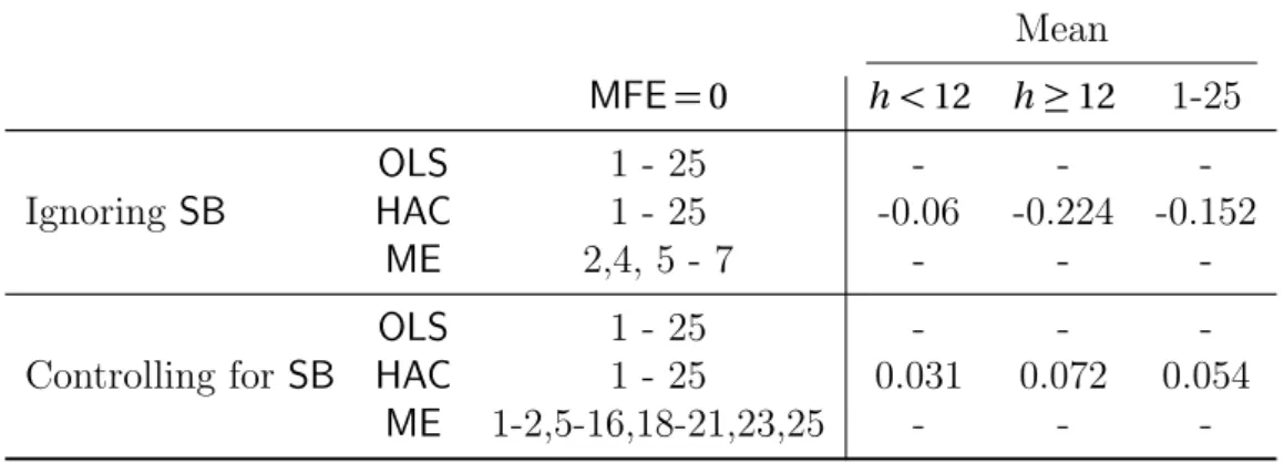
controlled for. Initially their seem to be a negative bias and not as many horizons for the ME bootstrap that are unbiased. This change however when controlling for SB, the MFE seem to be following the red dashed line. The 95% confidence interval for HAC does not change much however. A glance at table (4b) (page 24) conforms this, from only having five horizons that are unbiased and increase for unbiased horizons to 20. The mean of MFE also is reduced, from being negative to being close to zero and positive. When ignoring SB for some reason VECM is negatively biased for the longer horizon. Hence the model under-predicts the inflation rate.
Advantage in using the VECM is that it can describe the dynamic behavior of the time series analyzed. Intervention analysis can evaluate policy change and how one unit change in one variable changes the other.
5
Comparing the forecasts
Table (5) (page 24) compares all estimates that have a MFE equal to zero. When controlling for SB, the VECM produced forecasts had most horizons which are unbiased. ARIMA is closely behind the VECM by one ME bootstrap estimate less. For Riksbanken only seven horizons were unbiased when inference are made by the ME bootstrap. For OLS and HAC methods almost all of the results were unbiased. HAC however has a very wide 95% confidence interval. Another important conclusion to draw is that control for the presence of SB when forecasting, produces more unbiased estimation than for some reason just ignoring the presence of SB. In table (6) the mean of MFE for all method and short term versus long term are shown.
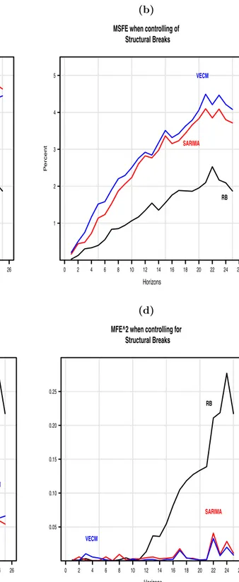
How is the precision then? Inspection on figure (4a) and (4b) (page 20), shows that the best precision18 is found for Riksbanken. The worst, when controlling for
SB is for VECM. The reason why is answered by decomposing the MSFE according to equation (2.8). Figure (4c) and (4d) (page 20), shows that when horizons are unbiased their MFE2 is almost constant over the horizons. This makes the MSFE
equal to the variance of the forecast horizon. Their is more movement in fig. 4c
than for when controlling for SB. The line for Riksbanken shows that after horizon 12 their is a sudden increase in the MSFE. But the overall is due to the variance for each horizon. Especially horizons 24, which is the peak for the MFE2.
6
Discussion
In this paper the MFE of Riksbanken were compared with the ones produced by econometric models. A further treatment were to compare the forecast when
controlling for the presence of SB and when for some reason the forecaster is ignorant of this fact. First of all when controlling for SB and not allowing it to affect the forecast does yield unbiased estimates. For the ME bootstrap the unbiased horizons increased considerably for both econometric models. In the context of precision not much happened for the VECM as it did for the seasonal ARIMA model. When not controlling for SB then ARIMA model systematically under-predicted and VECM over-predicted the inflation rate. Moreover not many horizons are unbiased. So when controlling for SB both ARIMA and VECM outperformed the Riksbanken in terms of unbiased horizons. Its likely that this happens because to omitted variable bias which causes biased and inconsistent estimates. The bias will persist even in large sample. This may be the reason for why the ME bootstrap yields more unbiased estimation since its satisfies the Ergodic Theorem19 when SB are removed.
When forecasting the inflation rate the Riksbanken has the most or best information set amongst all the forecaster. They use very advanced econometric models that are likely to yield better estimates than those analyzed in this paper. So from this viewpoint the bias resulted from the judgment of the executive board. A negative bias means that the forecast of the inflation rate has been systematically over-predicted and according to Clements and Hendry (2000) this would be due to that there is larger costs attached at being wrong at the other direction, that is under-predicting the inflation rate. This would mean that the loss function from Riksbanken is not symmetric. The same result were found for by Lundholm (2010) where, for longer horizons20 the positive bias had a a mean of MFE by 0.6 per cent.
Looking at table 6 this has been reduced to 0.3 meaning that the bias has been reduced. One consequence that may arise if Riksbanken sets its policy instrument based on information when the inflation rate is over-predicted for longer horizons, is that the repo rate also will be set to high than else necessary. This will result in lower output and higher unemployment rate. However the CPI as a measure may not be optimal and perhaps wage-inflation should be considered as target instead (Assarsson,2010, 57). CPI measures the total private consumption in the domestic market and a drawback is that it contains prices that are outside the control of Riksbanken (indirect taxes and subsidies) and prices that have perverse effects on monetary policy (mortgage interest cost) (Berg, 2000, 8). When Riksbanken raises the repo rate for decreasing the inflation rate the CPI can initial increase due the interest rate cost.
In a paper for the New Zealand’s central bank, Ranchhodinvestigated whether the forecast error from quarterly CPI inflation between 1992 and 2002 are unbiased for the central bank of New Zealand. Result showed that the current and 1 quarter ahead MFE are unbiased. The Reserve Bank had however consistently
under-19Which is a generalization of the Law of Large Numbers.
20Lundholm(2010) defines the forecast error asP
predicted the CPI for medium and longer horizons. Hence they view more cost in over-predicting the inflation rate and possibly setting the repo rate to low. In New Zealand the central-banks condition of employment depends on the target fulfillment, at the time being its hard to hold someone at the board responsible in Sweden for systematical deviation from target (Assarsson, 2010, 56).
The problem when forecasting with econometric models one has to thing about the so-called Lucas critique, which states that its naive to try to predict the effect of a change in economic policy entirely on the basis of relationships observed on historical data, especially highly aggregated historical data. Any change in policy will systematically alter the structure of econometric model (Lucas, 1976, 41). From the variable selection process it were clear that the GDP, Macro index, and Consumer Confidence Indicator are the variables that had the best predictive power on the inflation rate. Macro index is an index of that measures households purchasing plan and how the economy will evolve 12 months into the future. CCI measures the degree of optimism that consumers feel about the overall state at the economy and their personal financial situation. Hence those indices are important to follow as economic indicators for inflation rate. Here there might be some bias since selection of variables are based on the ability to collect data and select which variable that predicts the IR. Probably there is many more variables that are better candidates at forecasting the inflation rate.
References
Bengt Assarsson. Penningpolitiken i sverige 1995-2010. 2010. URL http://www.
ne.su.se/ed/pdf/39-3-ba.pdf.
Keith Bain and Peter Howells. Monetary Economics - Policy and its Theoretical Basis. palgrave Macmillan, 2009.
Claes Berg. Inflation forecast targeting: The swedish experience. (100), February 2000. URL http://ideas.repec.org/p/hhs/rbnkwp/0100.html.
Michael P. Clements and David F. Hendry. Forecasting Economic Time Series. Cambridge, 2000.
W Enders. Applied Econometric Time Series. Wiley, 2008.
Kerstin Hallsten and Sara T¨agtstr¨om. Beslutsprocessen - hur g˚ar det till n¨ar riksbanken ska best¨amma om repor¨antan. Penning – och valutapolitik, 2001 (1), 2001. URL http://www.riksbank.se/upload/Dokument_riksbank/Kat_
Robert Jr Lucas. Econometric policy evaluation: A critique. Carnegie-Rochester Conference Series on Public Policy, 1(1):19–46, January 1976. URL http://
ideas.repec.org/a/eee/crcspp/v1y1976ip19-46.html.
Michael Lundholm. Are inflation forecasts from major swedish forecasters biased? Research paper in economics 2010:10, Department of Economics, Stockholm University, 2010. URL http://swopec.hhs.se/sunrpe/abs/sunrpe2010_0010.
htm.
H L¨utkepohl. Applied Time Series Econometrics. Cambridge, 2004.
B Pfaff. Analysis of Integrated and Cointegrated Time Series with R. Springer, 2008.
Satish Ranchhod. Inflation forecast errors:preliminary findings. 2003. URL http:
//www.rbnz.govt.nz/research/forecastper/0133047.pdf.
Riksbanken. Inflationsrapport. Riksbanken, 2005(1), 2005. URL http://www.
riksbank.se/templates/ItemList.aspx?id=16028.
Riksbanken. Inflationsrapport. 2006(3), 2006. URL http://www.riksbank.se/
templates/ItemList.aspx?id=16028.
Lars E.O. Svensson. Evaluation monetary policy. Sveriges Riksbank, working pa-per series, Okt(235), 2009. URL http://www.riksbank.se/upload/Dokument_
riksbank/Kat_publicerat/WorkingPapers/2009/wp235.pdf.
Hrishikesh D. Vinod and Javier L´opez de Lacalle. Maximum entropy bootstrap for time series: The meboot R package. Journal of Statisticla Software, 29, January 2009. URL http://www.jstatsoft.org/v29/i05/paper.
Achim Zeileis. Econometric computing with hc and hac covariance matrix estimators. Journal of Statistical Software, 11(10):1–17, 11 2004. ISSN 1548-7660. URL
http://www.jstatsoft.org/v11/i10.
¨
Omer ¨Ozcicek. How important is variable selection for forecasting turkish inflation? Ege Academic Review, 1(2):61–72, 2001. URLhttp://ideas.repec.org/a/ege/
Appendix A: Graphs
Figure 1: Descriptive statistic
(a) The two second moments for the
forecast error of RB Target Dates P ercent −2.0 −1.5 −1.0 −0.5 0.0 0.5 1.0 1.5 2.0 2.5 3.0 3.5 4.0 1999 2000 2001 2002 2003 2004 2005 2006 2007 2008 2009 Variance Mean (b) Inflation rate and Repo rate
Time P ercent −0.5 0.0 0.5 1.0 1.5 2.0 2.5 3.0 3.5 4.0 4.5 1999 2000 2001 2002 2003 2004 2005 2006 2007 2008 2009 Repo Rate Inflation
Figure 2: MFE against horizon with 95 % Confidence Interval
Central Bank of Swedens MFE
Forecast Horizon (month)
MFE 5 10 15 20 25 − 2 0 2 4 HAC (Newey−West) OLS
Figure 3: MFE against horizon with 95 % Confidence Interval
(a) SARIMA:s MFE (white line)
Forecast Horizon (month)
MFE 5 10 15 20 25 − 2 0 2 4 HAC (Newey−West) OLS
Maximum entropy bootstrap
(b)
SARIMA:s MFE (white line) controlling for structural breaks
Forecast Horizon (month)
MFE 5 10 15 20 25 − 2 0 2 4 HAC (Newey−West) OLS
Maximum entropy bootstrap
(c) VECM:s MFE (white line)
Forecast Horizon (month)
MFE 5 10 15 20 25 − 2 0 2 4 HAC (Newey−West) OLS
Maximum entropy bootstrap
(d)
VECM:s MFE (white line) controlling for structural breaks
Forecast Horizon (month)
MFE 5 10 15 20 25 − 2 0 2 4 HAC (Newey−West) OLS
Figure 4: Estimating the precision using the MSFE according to eq. (2.8) and decomposing the MSFE according to eq. (2.8)
(a) MSFE when ignoring for
Structural Breaks Horizons P ercent 1 2 3 4 5 0 2 4 6 8 10 12 14 16 18 20 22 24 26 SARIMA VECM RB (b) MSFE when controlling of
Structural Breaks Horizons P ercent 1 2 3 4 5 0 2 4 6 8 10 12 14 16 18 20 22 24 26 SARIMA VECM RB (c) MFE^2 when ignoring for
Structural Breaks Horizons P ercent 0.05 0.10 0.15 0.20 0.25 0 2 4 6 8 10 12 14 16 18 20 22 24 26 SARIMA VECM RB (d) MFE^2 when controlling for
Structural Breaks Horizons 0.05 0.10 0.15 0.20 0.25 0 2 4 6 8 10 12 14 16 18 20 22 24 26 SARIMA VECM RB
Appendix B: Tables
Table 1: Testing eq. 2.4on et +h|T retrieved from RB
Mean
MFE= 0 h < 12 h ≥ 12 1-25
OLS 1 - 22 - -
-HAC 1 - 25 -0.015 -0.336 -0.195
-Table 2: Testing the predictive power of the variables
Variable Unit root test1 ∆π
t +1= ∆πt+ b(L)Xt+ �t +1
I(p) Drift F-stat F-Critical (Lags)2
Inflation1 1 No - -CCI.Index 1 No 4.138 3.047 (1) GDP 1 Yes 7.934 3.047 (1) Mikro.Index 1 No 4.385 3.047 (1) Makro.Index 1 No 4.803 2.657 (2) repo1 1 No 5.499 3.047 (1) Stibor.3M 1 No 3.409 3.047 (1) Gov.5Y 0 Yes 3.898 3.047 (1) ImportIndex 1 No 3.334 3.047 (1) M3 1 No 3.526 2.153 (5) UR1 0 No 3.38 3.047 (1) Tcw 1 No 3.488 3.047 (1) IF.Now 1 No 3.533 3.047 (1) IF.12M 1 No 4.186 2.657 (2)
1If I(1)and drift = Yes then the variable is a random walk with drift.
To make the variable a stationary process it has to be differenced once
2Lags start from 6 and the loop breaks when the p-value is less or
equal to the 5 per cent critical value, e.g., lag of 1 means that none of the lags were significant until lag 1 at the 5 per cent level
Table 3: Testing cointegration and control for serial correlation the following equation is used,∆ˆεt= a1εˆt−1+�ai +1∆ˆεt−i+ �t. If we reject the
null-hypothesis α = 0than we can conclude that the residual sequence are stationary and that the variable are cointegrated (Enders,2008, 374). A one indicates that the pairwise variables are cointegrated at the 5 per cent critical value.
(a) Unit-root test after the data selection
Without SB With SB I(p) Drift I(p) Drift
Inflation1 1 No 1 No GDP 1 Yes 1 No Makro.Index 1 No 0 No Stibor.3M 1 No 1 No UR1 0 No 1 No M3 1 No 1 No Tcw 1 No 1 No CCI.Index 1 No 0 No
(b)Testing pairwise cointegration.
Dependent variables IR GDP MA S.3M UR M3 TCW CCI IR - 0 0 0 0 0 0 0 GDP 0 - 1 1 0 0 0 0 MA 0 1 - 0 0 0 0 0 S.3M 0 0 1 - 0 0 0 0 UR 0 0 1 0 - 0 0 0 M3 0 0 0 0 0 - 0 0 TCW 0 0 0 0 0 0 - 0 CCI 0 0 1 1 0 0 0
-Table 4: Table for unbiased test
(a) Testing eq.2.4 on et +h|T retrieved from ARIMA
Mean MFE= 0 h < 12 h≥ 12 1-25 Ignoring SB OLS 1 - 25 - - -HAC 2 - 25 0.134 0.173 0.156 ME 18, 20 - 21 - - -Controlling for SB OLS 1 - 25 - - -HAC 1 - 25 0.029 0.088 0.062 ME 1,3,4,5,7,9,10-25 - -
-(b) Testing eq. 2.4on et +h|T retrived from VECM
Mean MFE= 0 h < 12 h≥ 12 1-25 Ignoring SB OLS 1 - 25 - - -HAC 1 - 25 -0.06 -0.224 -0.152 ME 2,4, 5 - 7 - - -Controlling for SB OLS 1 - 25 - - -HAC 1 - 25 0.031 0.072 0.054 ME 1-2,5-16,18-21,23,25 - -
-Table 5: Number of unbiased estimates for OLS, HAC corrected standard errors and the ME bootstrap methods
OLS HAC ME RB 22 25 7 ARIMA Ignoring SB 25 24 3 Controlling for SB 25 25 19 VECM Ignoring SB 25 25 5 Controlling for SB 25 25 20 1Testing the H
0 according to (2.5). More specific the test is all the estimates that has a
MFE= 0,∀ h ∈ {1,...25}. Here the total number of unbiased estimates are shown.
Table 6: The mean of MFE from the Riksbanken, VECM-model and ARMA model using equation (2.4)
Ignoring SB Controlling for SB
MFE h≤ 11M2 h≥ 12M 1-25 h≤ 11M h ≥ 12M 1-25
Riksbanken1 -0.015 -0.336 -0.195
VECM -0.06 -0.224 -0.152 0.031 0.072 0.054 ARIMA 0.134 0.173 0.156 0.029 0.088 0.062
1The Riksbanken is only calculated without controlling for the presence of SB in the
data
(a)Number of SB with the starting date at 1996:M1
Infla CCI.I GDP Mikro Makro repo1 Stibo Gov.5 Impor M3 UR1 Tcw IF.No IF.12 B 1 03-12 00-12 08-10 00-12 01-01 00-02 00-01 99-06 98-12 05-05 01-06 01-03 01-03 99-09 B 2 08-10 08-05 08-05 08-05 05-06 05-06 04-12 01-05 05-03 05-03 07-12 04-10
B 3 08-10 08-10 08-09 04-03 08-10 08-10 08-10
B 4 06-06
B 5 08-10
(b)Number of SB with starting date 1993:M6
Inflation1 GDP Makro.Index Stibor.3M UR1 M3 Tcw CCI.Index Break 1 1999-07 2008-07 2001-03 1996-03 1996-07 2005-11 1995-12 2001-01
Break 2 2008-05 2007-02 2001-08 2001-02 2008-05
Break 3 2005-03 2008-07
Cause Granger Instantaneous Grang Inst Grang Inst Grang Inst Grang Inst IR 2.262 10.019 2.277 11.727 2.606 2.652 2.679 2.155 3.308 1.106 GDP 3.049 46.001 2.777 43.38 2.807 43.167 3.247 42.939 2.004 8.771 MA 2.102 69.385 2.626 65.49 2.635 64.72 2.473 58.327 2.824 57.786 S.3M 1.119 11.863 0.997 15.166 - - - -UR 1.457 40.076 1.128 40.629 1.186 40.669 1.191 39.393 - -M3 1.75 7.35 - - - -TCW 0.903 35.71 0.72 30.726 0.374 28.771 - - - -CCI 4.007 57.966 5.842 56.601 6.533 55.992 6.652 56.218 8.358 55.702 Other VAR(p)2 4 - 3 - 3 - 3 - 3 -F-stat1 1.484 - 1.612 - 1.675 - 1.762 - 1.892 -χ21 14.067 - 12.592 - 11.07 - 9.488 - 7.815
-1The F-statistic and theχ2 has a critical value at the 5 per cent level
2Lag length is determined by Akaike information criterion (AIC)
3The Granger and Instantaneous statistics is obtained by using the bootstrap technique, with 1000 replication 4The Granger test hypothesis is H
0: y2t do not Granger-Cause the other variables and for the instantaneous test H0: No instantaneous causality betweeny2t and the other variables
couraging guidance, insightful comments, support during the writing of this thesis and helping me into exploring reproducible econometrics.
Abstract
The focus of this paper is to evaluate if forecast produced by the Central Bank of Sweden (Riksbanken) for the 12 month change in the consumer price index is unbiased? Results shows that for shorter horizons (h < 12) the mean forecast error is unbiased but for longer horizons its negatively bi-ased when inference is done by Maximum entropy bootstrap technique. Can the unbiasedness be improved by strict ap-pliance to econometric methodology? Forecasting with a linear univariate model (seasonal ARIMA) and a multivari-ate model Vector Error Correction model (VECM) shows that when controlling for the presence of structural breaks VECM outperforms both prediction produced Riksbanken and ARIMA. However Riksbanken had the best precision in their forecast, estimated as MSFE.
Keywords: Inflation rate, VECM, Structural Breaks, Rolling-event forecast, Maximum Entropy bootstrap, ARIMA
1 Programming and forecast 1
2 Econometric Method 1
2.1 Unit root-test . . . 1
2.2 SB and Cointegration . . . 3
3 Model building 5
3.1 Vector Error Correction Model (VECM) . . . 5
3.2 Granger- Causality Analysis . . . 8
3.3 Forecast . . . 9 4 ARIMA- model 10 Appendix A: Tables 12 Appendix B: Graphs 23
List of Figures
1 Data transformation . . . 24 2 Forecast . . . 251
Programming and forecast
This paper is written with the help of Docstrip, which allows for many documenta-tions in a single Rnw-file. Since the task for solving this papers purpose involves many loops and functions written in R-code, it essentials to make Sweave work as fast as possible. Hence I make use of RData-files. More explicit, I write R-codes and save these in a RData-file. In the Rnw-file I only load the latest RData-file that con-sist of all the object up until the most recent work. For example in the accompanied file ”rcode.pdf”, where all the R codes are shown, in line 1004 I use save() and in line 1010 a new file called ”arma.R” is created. Then from line 1010 and onwards to 1175 is only forecasting with the univariate model Autoregressive Integrated Moving Average (ARIMA). In Sweave only the last RData-file is loaded which contains all the object created shown in ”rcode.pdf”. As text-editor GNU Emacs are used and everything is written in LATEX mode.
The next step is to download the inflation rate (IR) from the Riksbanken (RB), a vector of prediction Predicted (P) with starting date 1999-06. Data is downloaded and each vector is taken together from different xls-files downloaded from RB. Before 2005 these report was published 4 times a year along with there forecast, after 2006 this was reduced to 3 times a year. Due to the financial crisis late 2007 there is a follow-up report approximately two months after each report. I will use the last of these reports data to test the FE. Another change is that the forecasting horizon has increased from approximately two years to three years. For comparability reasons I reduce each forecast horizon to 25 observations. Since the there is no follow-up in year 2006 I need to interpolate the last quarter of this year. I use will the R-function na.approx(), which is a linear function. Results for RB if whether the estimates are unbiased or not are shown in table (2) (page13), and for ARIMA and VECM in table (3), (4) (page 14, 15) respectively. These estimates are done with function BiasTest() in ”rcode.pdf” line 154.
2
Econometric Method
2.1
Unit root-test
Assuming that there is no structural breaks than the Augmented Dickey-Fuller (ADF) test suffice for detecting whether there is a stochastic trend or deterministic trend.
The test procedure is the following (Pfaff, 2008, 94): ∆yt= β1+ β2t + πyt−1+ k � j =1 γj∆yt−j+ u1t, (2.1a) ∆yt= β1+ πyt−1+ k � j =1 γj∆yt−j + u2t, (2.1b) ∆yt= πyt−1+ k � j =1 γj∆yt−j+ u3t (2.1c)
where the summation term is for controlling any serial correlation. In equation (2.1a), the null-hypothesis is: H0: φ3= (β1,β2,π) = (β1,0,0), which means that there
is no deterministic trend, but suspected stochastic trend. If H0 cannot be rejected
as listed in φ3 and τ3= (π) = 0, then the series has a suspected unit-root. Moving
on too test if the series is a random walk with or whit out drift, the null-hypothesis is H0: φ2= (β1,β2) = (β1,0). If H0 rejected then a conclusive answer is that the series
behaves as a pure random walk. Next we proceed to equation (2.1b) based on τ3
test. For the sake of completeness, it is now tested whether this model contains a drift or not. The null-hypothesis is H0: τ2= (β1,π) = (β1,0) if β1�= 0 and π = 0
than the variable is a random walk with drift. In the last equation (2.1c), testing if the series are a pure random walk is made only to amplify the inference drawn under (2.1b). If H0: τ1= 0 than the series is a pure random walk. Lastly a test for
determining the order of integration is done, and we reestimate (2.1a) and continue the the process mentioned above. If we can reject the null-hypothesis and accept H1:= π �= 0the series is said to be of order one (I(1)). Results are displayed in table
(5) and (6b) for the differenced data. The critical values is shown in table (6a). A problem that might occur is if there is a structural break in the variable. Then the ADF-test may have very low power if the shift is simply ignored (L¨utkepohl, 2004, 58).
The only difference when testing for unit-root with and without Structural Breaks (SB) is for the variables CCI.Index, Makro.Index, UR1 . With SB in the variable Consumer Confidence Indicator (CCI) is considered to be a I(0) process and without SB its a I(1) process, the same applies for the Macro index (MA). The contrary is for the Unemployment Rate (UR) were initially the variable is considered to be a Integrated of order one (I(1)) process but after removing the SB its a I(0) process. The test for the unit-root test is concisely described in the below enumerate.
(1) inflation rate has a φ3 and τ3 lower than the critical value in table 6a. The
walk. τ1 is in the region of accepting that the H0= 0. In table 6b testing which
order of integration the variable is, shows IR is I(1). This means that in order to make it stationary it has to be difference once.
(2) The Consumer Confidence Indicator has a φ3 and a τ3 that is inside the
accepting region for the H0. Since τ1 is between the 10 and 5 per cent region
CCI is a pure random walk. From table (6b) it clear that the variable is a I(1)
process (even its only at the margin, continuing the ADF test conforms that the first difference makes the data stationary).
(3) Gross Domestic Product Has aφ3 andφ1 over the critical value. τ1 shows that
we cannot reject H0, hence the variable is a random walk with drift and a I(1)
process.
(4) The Mikro.Index, repo rate is both pure random walks and I(1). (5) Stibor rate is a pure random walk and a I(1)process.
(6) Government bonds (5 year) is stationary and hence a Integrated of order zero (I(0)) process.
(7) Import Price Index Money supply (M3) and Total Competitiveness Weights (TCW) are pure random walks and I(1)process.
(8) The Unemployment Rate has a τ1 equal to -2.722, which makes it a I(0)process.
The cointegration process for the VECM specification is presented in section (2.2). The unit-root test for those variables, with and without controlling for Structural Breaks is presented in tables (7a) and (7b) (page18). The main difference is found the Gross Domestic Product (GDP) which should be a random walk with drift (see graph 1b (page24), but the test with a SB concludes that there is no such positive drift. For MA the one with SB conclude that the variable is a I(0) but without SB its a I(1)process.
2.2
SB and Cointegration
The procedure to detect any SB is done with the following linear model1
(2.2) xt = β0+ β1t + 12
�
i =1
βiSi t+ �t,
where β1 is the trend coefficient, and βi for i ∈ {1,2,...,12}are the parameters for
the seasonal dummies where the reference category is for month 12. Then using (2.2) for detecting any SB is done with the following regression model
(2.3) xt = β0+ β1t + 12 � i =1 βiSi t+ B � b =1 αb 0+ αb 1t + 12 � i =1 αb iSt b Db t+ �t,
where Db t, b = 1,...,B are dummy variable dividing data. B is the optimal number
of breaks2. If there is any SB its removed and the following variable are the one
that will be in the continuing of the study: (2.4) xt= ˆβ0+ ˆβ1t + ˆ�t.
This is done by a regression procedure and presented in the thesis.
The Engle-Granger methodology propose a four step procedure to determine if two variables are cointegrated. Here I report only two of those steps since Johansen procedure is the test when considering multi-dimensional equations like a VECM or Vector autoregression (VAR).
Step 1 Cointegration necessitates that two variables be integrated of the same order. The ADF can be used. This is done i table (5). If the variables are of different order it is possible to conclude that they are not cointegrated. Step 2 Estimate the long-run equilibrium (Equilibrium refers to a long-run
rela-tionship among non stationary variables) relarela-tionship in the form (2.5) yt = β0+ β1zt+ εt
In order to determine if the variables are cointegrated the residual{ˆε}in (2.5) will contain the deviation from the long-run relationship. If these deviations are found to be stationary then the sequence are cointegrated. The ADF suffice for testing this, more formally we test the following equation: (2.6) ∆ˆεt = α1εˆt−1+
n
�
i =1
αi +1∆ˆεt−i+ �t
where the H0 is that α = 0 the residual sequence is not stationary, hence if
we reject the null-hypothesis that α = 0 and the variables are cointegrated.
Since the aim is only to test the pair of the variable the explanation suffice for this purpose, Enders (2008, see, 374 for more) The chosen variable from the selection section is shown in the first column at table (7a). This selection process was done with R-function line 115 in “rcode.pdf”.
In table (8) testing the selected variables for pairwise cointegration is done. The pairwise cointegration is found for the TCW with GDP, acma and the UR. For the Stibor.3M (S.3M) cointegration is found between GDP and MA. Thus, a Rank (rk) test is necessary to determine how many cointegration vector there is in the matrix. But this will be done on the final selected variables, which is tested with the methods of Granger Causality.
The rk test on final selected variables is for the IR, GDP, MA and CCI and yields the following test statistic shown in table (11) (page 21). The length of significant for a rank of 1 is 30 out of the 40 observation. And for the eigen test is 29 out of the 40 observation. Test are explained more in depth in section (3). In line 203 function vec.test for this purpose is shown and in 1222 and 1226 the selection codes are shown (object r1 and r2).
3
Model building
3.1
VECM
Since the cointegration section showed that there is one cointegrating vector the concept of VECM is explained here. First some important notes in the matrix algebra concept that is related to the VECM.
Definition 1 (Conditions for nonsingularity). A sufficient condition for the non-singularity of a matrix is that its rows (columns) to be linear independent. When the dual condition of squareness and linear independence (see definition below) are taken together, they constitute the necessary–and–sufficient condition for nonsingu-larity (nonsingunonsingu-larity ⇔squareness3 and linear independence). When matrix A
is nonsingular, which means that the inverse A−1 does exist then a unique solution x=A−1d can be found.
Definition 2 (Linear Independence). The n vectors a1,a2,...,an in �m are linear
dependent if there exist numbersc1,c2,...,cn not all zero, such that
(3.1) c1a1+ c2a2+ ··· + cnan= 0
If this equation holds only in the “trivial” case when c1= c2= ··· = cn= 0, then the
vectors are linearly independent.
Theorem 1. The n column vectors a1,a2,...,an of the n× n matrix A= a11 a12 ... a1n a21 a22 ... a2n ... ... ... ... an1 an2 ... ann , where aj = a1j a2j ... an j (3.2)
are linearly independent if an only if |A| �= 0.
Thus, if the rows in A is linearly independent, the determinant must have a nonzero value. The discussion of nonsingularity can now be summarized. Given a linear equation system Ax= m a t d, where A is a (n × n) coefficient matrix,
|A| �= 0 ⇔ there is row (column) indepence in matrix A
(3.3)
⇔ A Is nonsingular
⇔ A−1exist
⇔ a unique solution x=A−1d exits
Definition 3 (Rank). The rk of a matrix A is defined to be the maximum number of linearly independent rows (columns) in A. The rk of an (m × n) matrix can at most be m or n, whichever is the smallest. Symbolically, this fact may be expresed as follows:
(3.4) r (A) ≤ min{m ,n}
which is read “The rk of A is less than or equal to the minimum of the set of two numbers m and n”. The rk of an (n × n) nonsingular matrix A must be n, in that case we write r (A) = n.
Definition 4 (Eigenvalues and eigenvectors). Suppose that there is a scalarλwith the special property that
(3.5) Ax= λx
A nonzero vector x that solves (3.5) is called eigenvector, and the associated λis called an eigenvector. It should be noted that if x is an eigenvector associated with the eigenvalue λ, then so is αx for every scalar α�= 0. Eigenvalues and eigenvectors are also called characteristic roots (values) and characteristic vectors, respectively. The way to find eigenvalues is to rewrite equation (3.5) as
This homogeonous linear system of equations has a solution x�= 0 iff the coefficient matrix has determinant equal to zero – that is, iff|A−λI| = 0. Lettingp (λ) = |A−λI|, where A= (ai j)n×n, we have the equation
(3.7) p (λ) = |A− λI| = � � � � � � � � � a11− λ a12 ... a1n a21 a22− λ ... a2n ... ... ... ... an1 an2 ... ann− λ � � � � � � � � � = 0
This is the characteristic equation (or eigenvalue equation) of A. The poly-nomial p (λ) is called the characteristic polynomial of A. It follows from (3.7)
that p (λ) is a polynomial of degreen inλ. Thus it has n roots (real or complex).
The rk for the dataset is determined by first estimating the lag length with the R function VARselect(). Then rk is evaluated by ca.jo() in png vars, which decided the Rank. Estimate are shown in table (11) (page 21).
(3.8) ∆yt= Πyt−1+
p−1
�
i =1
Γ∆yt−1+ ΨDt+ �t
Where ∆yy−1 is the I(1) variables and sometimes called the long-run or long-term
parameters, andΓj the short term parameters. If a VAR has unit-roots4 the matrix
Π = −(Ik− A1··· − Ap) is singular. Suppose rk(Π) = r, then Π can be written as a
product of (K × r ) matrices α and β with r(α) =rk(β ) = r. As follows Π = αβ�. Premultiplying an I(0)vector by some matrix results again an I(0) process. Thus,
β�yt−1 is I(0)and contains the Co-integrations relations among the components of yt. The rank of Πis therefore reffered to as the cointegration rank of the system
andβ is a cointegration matrix. For example, if there are three variables with with two cointgrations relations (r = 2) we have
Πyy−1= αβ�yt−1= α11 α12 α21 α22 α31 α32 � β11 β12 β13 β21 β22 β23 � y1,t−1 y2,t−1 y3,t−1 (3.9) = a11e c1,t−1+ a12e c2,t−1 a21e c1,t−1+ a22e c2,t−1 a31e c1,t−1+ a32e c2,t−1 , where e c1,t−1= β11y1,t−1+ β21y2,t−1+ β31y3,t−1 4 that is det(I k− A1z− ··· − Apzp) forz = 1
and
e c2,t−1= β12y1,t−1+ β22y2,t−1+ β32y3,t−1
The matrixα is sometimes called the loading matrix. It contains the weights attached to the cointegrating relations in the individual equations of the model (L¨utkepohl, 2004, 89-91).
Testing the rk is done by the following two statistics:
λtrace(r ) = −T n � i =r +1 ln(1 − ˆλi) (3.10) λmax(r,r + 1) = −Tln(1 − ˆλr +1) (3.11)
where ˆλi is the eigenvalues obtained (Enders, 2008, 391). Equation (3.10) tests the
null-hypothesis that the number of distinct cointegrating vectors is less than or equal to r, more formally
H0: r = 0 against H1: r = 1,2,...
(3.12)
For equation (3.11) the null-hypothesis is that th number of cointegrating vectors is r against the alternative r+1, more formally:
H0: r = 0 against H1: r = 1
(3.13)
3.2
Granger- Causality Analysis
Causality is important since the aim is to find a model that will produce a forecast with the least MFE. If a variable y2t to be causal for variable y1t the former helps
to improve the forecast to the latter. Denoting y1,t +h|Ωt the optimal h-step forecast
of y1t at origin t based on the set of all the relevant information in the universe
Ωt, y2t is defined to be Granger-noncausal for y1t iff (L¨utkepohl, 2004, 144):
(3.14) y1,t +h|Ωt= y1,t +h|Ωt\{y2,s|s≤t } h = 1,2,...
where the symbol � \� denotes the set of all elements of a set � not contained in the set �. Thus, in (3.14) y2t is not causal for y1t, if removing the past of y2t
from the information set does not change the optimal forecast of y1t at any forecast
horizon. In turn, y2t is Granger-Causal fory1t if (3.14) does not hold for at least
one h, and thus a better forecast of y1t is obtained by including the past ofy2t in