Institutionen för energi och teknik Report 030
Department of Energy and Technology ISSN 1654-‐9406
Green nitrogen -‐ possibilities for
production of mineral nitrogen
fertilisers based on renewable
resources in Sweden
Serina Ahlgren
Andras Baky
Sven Bernesson
Åke Nordberg
Olle Norén
Per-‐Anders Hansson
SLU, Sveriges lantbruksuniversitet
Fakulteten för naturresurser och lantbruksvetenskap Institutionen för energi och teknik
Swedish University of Agricultural Sciences Department of Energy and Technology
Green nitrogen -‐ Possibilities for production of mineral nitrogen fertilisers based on renewable resources in Sweden
Serina Ahlgren, Andras Baky, Sven Bernesson, Åke Nordberg, Olle Norén, Per-‐Anders Hansson
Photographies frontpage: Serina Ahlgren and Bioenergiportalen Report 030 ISSN 1654-‐9406 Uppsala 2011
Institutionen för energi och teknik Report 030
Department of Energy and Technology ISSN 1654-‐9406
Green nitrogen -‐ possibilities for
production of mineral nitrogen
fertilisers based on renewable
resources in Sweden
Serina Ahlgren
Andras Baky
Sven Bernesson
Åke Nordberg
Olle Norén
Per-‐Anders Hansson
ABSTRACT
The production of mineral nitrogen is one of the largest fossil energy inputs in Swedish agriculture. However, mineral nitrogen can be produced based on renewable energy. This would lower the dependency on fossil energy in food production.
This project investigated the possibilities and the consequences for the Swedish agricultural sector of producing nitrogen from renewable resources and agricultural raw materials. More specifically, it studied the land use, energy use and greenhouse gas emissions from the production of ammonium nitrate based on wind power, biomass-based combined heat and power (CHP) and thermochemical gasification of biomass. Ammonium nitrate was chosen since it is the most commonly used nitrogen fertiliser in Sweden. The study also compared small-scale and large-scale production and estimated the production costs.
The construction of new plants and integration within existing biomass heat and power production were compared. For many of the scenarios studied, all the technology needed is already available on a commercial basis and production is a matter of combining the different stages.
The production costs based on small-scale wind power were an estimated 43 SEK/kg N. The costs for large-scale production based on biomass combustion were an estimated 8 SEK/kg N, which is very competitive compared with the fossil-based alternatives on the market today. However, the cost estimations were very rough and associated with large uncertainties. More detailed economic modelling and calculations are needed to support any future investment decisions.
The greenhouse gas modelling was performed using life cycle assessment methodology. The results showed that in most of the scenarios studied, greenhouse gas emissions and use of fossil energy can be significantly lowered. The exception was integration of nitrogen production into existing biomass-fired heat and power production, since the reduced electricity output was assumed to be compensated for by marginal coal power.
Using green nitrogen in crop production can substantially lower the energy and carbon footprint of crops. Using these crops for production of biofuels can also lower the carbon footprint of the biofuels, making the comparison to fossil fuels more favourable for biofuels. In conclusion, greenhouse gas emissions and fossil energy use can be lowered and there seem to be no technological or economic obstacles to producing green nitrogen. Therefore supplying green nitrogen to agriculture should be a high-priority activity, as nitrogen is one of the pillars for food and bioenergy security of supply. However, it is very difficult to make general recommendations on choice of technology and raw materials, since this choice is dependent on the context. Therefore each case much be carefully investigated and the raw material checked for its sustainability.
SAMMANFATTNING
Tillverkning av mineralkväve är en av de största insatserna av fossil energi i det svenska jordbruket. Mineralkväve kan dock produceras baserad på förnybar energi, vilket innebär att beroendet av fossil energi i livsmedelsproduktionen kan minska.
Syftet med detta projekt var att undersöka möjligheterna och konsekvenserna för den svenska jordbrukssektorn om kväve producerades från förnybara resurser. Mer specifikt var syftet att studera markanvändning, energianvändning och utsläpp av växthusgaser från produktionen av ammoniumnitrat baserad på vindkraft, biomassabaserad kraftvärme och termokemisk förgasning av biomassa. Ammoniumnitrat valdes eftersom det är det vanligaste enkla kvävegödselmedlet i Sverige. Syftet var också att jämföra småskalig och storskalig produktion och att uppskatta produktionskostnader.
Både nybyggda anläggningar och integration inom befintlig biomassabaserad kraftvärme har studerats. För många av de studerade systemen finns alla de teknikdelar som behövs redan i kommersiell skala, det är en fråga om att sätta ihop bitarna.
Kostnaden för produktion baserad på småskalig vindkraft beräknades till 43 kr/kg N. Kostnaden för storskalig produktion baserad på förbränning av biomassa beräknades till 8 kr/kg N vilket är mycket konkurrenskraftigt jämfört med fossila alternativ på marknaden idag. Kostnadsuppskattningarna är dock mycket grova och försedda med stora osäkerheter. Mer detaljerad ekonomisk modellering och beräkningar behövs för att stödja eventuella investeringsbeslut.
Modellering av växthusgasutsläpp gjordes med livscykelanalysmetodik. Resultaten visade en minskning av växthusgaser och användning av fossil energi. Undantaget var integrationen av kväveproduktionen i befintligt kraftvärmeverk, eftersom den minskade elproduktionen antogs kompenseras med kolkraft.
Att använda grönt kväve i växtodling kan minska energiåtgången och växthusgasutsläppen markant. Om grödorna används för att producera biodrivmedel kan dessutom klimatavtrycket för biodrivmedlen också minska, vilket ytterligare ökar reduktionen av växthusgaser jämfört med fossila drivmedel.
Sammanfattningsvis kan sägas att växthusemissionerna och fossilenergianvändningen kan sänkas och det verkar inte finnas några tekniska eller ekonomiska hinder för att börja producera grönt kväve. Vi hävdar att grönt kväve till jordbruket bör vara en prioriterad aktivitet eftersom kväve är en av grundpelarna för en trygg försörjning av mat och bioenergi. Det är dock svårt att ge generella rekommendationer om val av teknik och råvaror till produktion av grönt kväve, eftersom det till stor del är beroende på sammanhanget. Varje fall måste mycket noggrant undersökas och råvaror bör vara hållbart producerade.
ACKNOWLEDGEMENTS
This project was carried out with financial support from Stiftelsen Lantbruksforskning – The Swedish Farmers’ Foundation for Agricultural Research, to whom we express our thanks. We would also like to thank Christian Hulteberg (CEO, Biofuel-Solution) and Klaus Noelker (Head of Process Department Ammonia and Urea Division, Udhe) for participation in the project. They provided input to the scenario construction and discussions and took the time to participate in a meeting in Uppsala.
1 INTRODUCTION ... 1
1.1 Energy use in Swedish agriculture ... 1
1.2 Greenhouse gas emissions from Swedish agriculture ... 2
1.3 Aims and objectives ... 2
2 BACKGROUND TO NITROGEN FERTILISERS ... 4
2.1 The beginning of nitrogen fertilisers in agriculture ... 4
2.2 Present use of nitrogen fertilisers ... 4
2.3 Future use of nitrogen fertilisers ... 6
2.4 Production of ammonia ... 6
2.5 Production of fertiliser products ... 9
2.6 Production of ammonia based on renewable energy ... 10
3 METHODS ... 11
3.1 Scenario construction ... 11
3.2 General introduction to life cycle assessment methodology ... 11
3.3 Chosen impact categories in the study ... 12
3.4 Functional unit in the study ... 13
3.5 Overview of scenarios studied ... 13
3.6 System boundaries and delimitations ... 15
3.7 Production costs ... 16
4 INVENTORY OF ENERGY AND EMISSION DATA ... 18
4.1 Wind power ... 18
4.2 Cultivation/collection of biomass raw material ... 18
4.3 Land use and soil carbon ... 18
4.4 Transport of biomass raw material ... 20
4.5 Nitrogen fertiliser production ... 21
4.6 Energy credit/debt ... 22
4.7 Replaced fossil nitrogen fertiliser ... 22
5 INPUT DATA FOR ESTIMATION OF PRODUCTION COSTS ... 23
5.1 Wind power ... 23
5.2 Power generation in CHP ... 23
5.3 Electrolysis and hydrogen storage ... 24
5.4 Ammonia production and storage ... 25
5.5 Nitric acid production ... 25
5.6 Mineral fertiliser plant ... 26
6 RESULTS ... 27
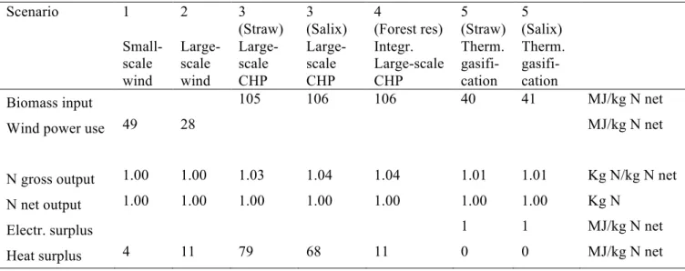
6.1 Plant inputs and outputs ... 27
6.2 Transport distance biomass ... 28
6.3 Land use ... 28
6.4 Energy ... 28
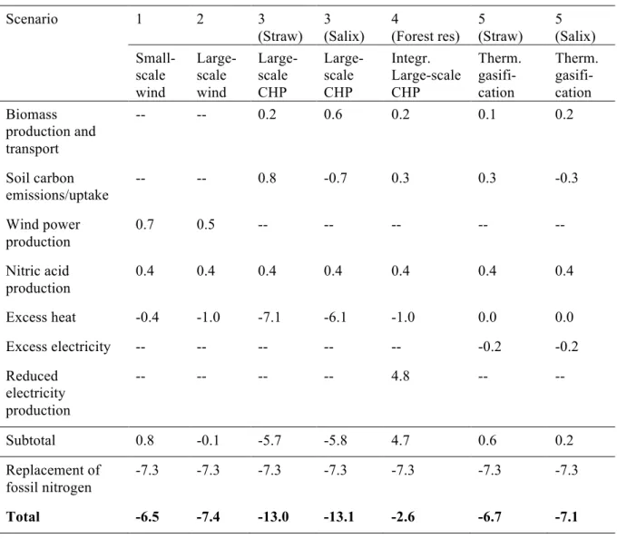
6.5 Greenhouse gas emissions ... 29
6.6 Production costs ... 30
7 SENSITIVITY ANALYSIS ... 32
7.1 Greenhouse gas emissions ... 32
7.2 Production costs ... 36
8 DISCUSSION ... 38
8.1 Uncertainties associated with LCA modelling ... 38
8.2 Best use of renewable resources ... 38
8.3 Cost of production and price competitiveness ... 39
8.4 Supply Swedish agriculture with green N? ... 42
8.5 Using green fertilisers in crop production ... 42
8.6 Effects on biofuel energy balance and GHG emissions ... 45
9 CONCLUSIONS ... 48
10 REFERENCES ... 49
APPENDIX A. TECHNICAL DESCRIPTION OF ELECTROLYSIS SCENARIOS ... 55
APPENDIX B. TECHNICAL DESCRIPTION OF THERMAL GASIFICATION ... 60 Contents
1 INTRODUCTION
Nitrogen fertilisers are needed in agriculture to obtain high yields of agricultural crops. Large-scale use of mineral* nitrogen fertilisers began after Second World War and without this, the
expansion of the world population would have been impossible (Smil, 2001).
Nitrogen gas accounts for 78% of the volume of our atmosphere. However, converting it to a form that is useful for agriculture costs energy. At present, the production of nitrogen fertiliser accounts for 1.2% of global primary energy demand (IFA, 2009a). Production is most commonly based on natural gas, but gasification of coal and heavy oil also occurs.
In other words, the production of mineral nitrogen fertilisers is based on fossil fuel resources. In the long run, this is not a sustainable solution as the fossil fuels will run out sooner or later. The use of fossil fuels also contributes to global warming, which is believed by many to be the largest threat to mankind. In this report, alternative ways of producing mineral nitrogen fertilisers are investigated.
1.1 Energy use in Swedish agriculture
At present, the total use of energy in Swedish agriculture is estimated to be 9.2 TWh (33 PJ) per year (Figure 1). The energy use can be divided into two parts, direct and indirect. The direct energy is the energy used on farms, while the indirect energy is the energy used for producing purchased inputs, although not including the production of machinery and buildings.
Figure 1. Direct and indirect use of energy in Swedish agriculture (Ahlgren, 2009).
The largest direct energy use is the use of fossil diesel (primarily for tractor fuel). Fossil oil and solid biofuels (mainly wood products and straw) are used for heating animal houses and drying grain (SCB, 2008). Electricity is primarily used in animal production. The Swedish electricity production mix consists mainly of hydro and nuclear power and only 7% is based on fossil energy.
* The term “mineral nitrogen” is here used to describe industrially produced nitrogen, differentiated from
“organic nitrogen” which is present in for example soil organic matter, crop residues and manures. Organic nitrogen can be mineralised by microbes to plant available forms (ammonium and nitrate) but in this study we only study the mineral nitrogen produced by industrial processes.
Direct energy use 5,9 TWh
Diesel 48% O il 13% Electricity 18% Solid biofuels 20% Liquid biofuels 1%
Indirect energy use 3.3 TWh
Artificial fertilisers 56%
Pesticides 5% Seed 1%
Transport of inputs 4%
Direct energy use 5.9 TWh
Diesel 48% O il 13% Electricity 18% Solid biofuels 20% Liquid biofuels 1% Silage plastic 7% Imported fodder 27% Direct energy use 5,9 TWh
Diesel 48% O il 13% Electricity 18% Solid biofuels 20% Liquid biofuels 1%
Indirect energy use 3.3 TWh
Artificial fertilisers 56%
Pesticides 5% Seed 1%
Transport of inputs 4%
Direct energy use 5.9 TWh
Diesel 48% O il 13% Electricity 18% Solid biofuels 20% Liquid biofuels 1% Silage plastic 7% Imported fodder 27%
The largest indirect energy use is the production of fertilisers. The energy used for fertiliser production is largely due to production of nitrogen fertilisers, the main energy carrier being natural gas. The energy consumption for nitrogen production was assumed here to be 39 MJ (11 kWh) per kg N, which is an average European figure based on Jenssen and Kongshaug (2003). To a large extent the other indirect energy inputs are also based on fossil resources, for example silage plastic and the production of imported fodder.
1.2 Greenhouse gas emissions from Swedish agriculture
According to the Swedish national inventory report (Naturvårdsverket, 2009), greenhouse gas (GHG) emissions from Swedish agriculture amounted to 8.43 million metric tonnes (ton) CO2-equivalents during 2007, corresponding to 13% of national greenhouse gas emissions.
This is mainly from animal production (methane) and soil emissions (nitrous oxide). However, that figure does not include the production of inputs such as diesel, fertilisers and imported fodder, nor carbon dioxide release from organic soils.
In a study by Engström et al. (2007), the emissions of GHG from the entire food chain, including the food industry, exports and imports, was calculated to be about 14 million ton CO2-equivalents. In another study, conducted by the Swedish Board of Agriculture (SJV,
2008a), the GHG emissions from agriculture were estimated to be 15 million ton CO2
-equivalents per year, the largest contribution coming from nitrous oxide emissions from soil (Table 1). However, that report points out the large uncertainties in these quantifications, especially for the nitrous oxide emissions from soil and the carbon dioxide emissions from managed organic soils.
Table 1. Distribution of greenhouse gas emissions from Swedish agriculture (SJV, 2008a)
Activity % of total
Nitrous oxide from nitrogen in soil 30%
Carbon dioxide from managed organic soils 25%
Methane from animal digestion 20%
Production of mineral fertilisers 10%
Methane and nitrous oxide from manure (storage and spreading) 7%
Carbon dioxide from fossil fuels 7%
Imported feed 3%
As can be seen in Table 1, the production of fertilisers accounts for only 10% of the GHG emissions from agriculture. However, some of the other larger items are emissions that are steered by biological activities and therefore difficult to control. In the nitrogen fertiliser production system there is a practical possibility to lower the GHG emissions. On a global scale, the production of nitrogen fertilisers is calculated to represent about 1% of anthropogenic GHG emissions (IFA, 2009a).
1.3 Aims and objectives
The general aim of this project was to investigate the possibilities and the consequences for the Swedish agricultural sector of producing nitrogen from renewable resources and agricultural raw materials. Specific objectives were to study the land use, energy use and GHG emissions from the production of ammonium nitrate based on wind power, biomass combined heat and power (CHP) and thermochemical gasification of biomass (Figure 2).
Ammonium nitrate was chosen since it is the most commonly used nitrogen fertiliser in Sweden*. An additional aim was to compare small-scale and large-scale production and to estimate the production costs.
Figure 2. The nitrogen fertiliser production routes studied in this report. CHP: Combined heat and power.
* Also sold as calcium ammonium nitrate which is produced in the same way as ammonium nitrates but with
calcium added in the last step
Biomass! Ammonia production! Hydrogen production via electrolysis! Thermo-chemical gasification! Electricity/heat production (CHP)! Electricity production (wind power)!
Gas cleaning and hydrogen production! Biomass! Wind! Ammonium nitrate production! Nitric acid production!
2 BACKGROUND TO NITROGEN FERTILISERS
2.1 The beginning of nitrogen fertilisers in agriculture
Since the beginning of agriculture, cultivation of leguminous crops and recycling of organic waste has been a method for soil and nutrient conservation. However, it was not until the early 19th century that Justus von Liebig discovered nitrogen’s role for crop productivity.
Once this was clearly understood, the quest for new sources of nitrogen began. Bird excrement (guano) from a few tropical islands and sodium nitrate deposits in South America were found to have 30 times higher nitrogen content than common manure and were used as fertilisers. However, the demand was high and these resources were rapidly exhausted (Smil, 2001; Erisman et al., 2008).
During the second half of the 19th century nitrogen fertiliser production started from recovery of ammonia from the coking of coal, from calcium cyanamide and from fixation of atmospheric N2 by electrical discharge. Fritz Haber was born 1868 in Germany. During the
beginning of the 20th century, Fritz worked at the Technische Hochschule in Karlsruhe and started his research on ammonia synthesis. In 1909 he developed a laboratory scale high pressure ammonia synthesis working over an iron catalyst combining hydrogen and nitrogen gas. However, it was Carl Bosch who took the invention to commercial scale; today known as the Haber-Bosch process. The fuel and feedstock for the first commercial ammonia plant, situated in German Oppau, was coal. Since then, the use of nitrogen fertilisers has steadily increased (Smil, 2001).
2.2 Present use of nitrogen fertilisers
Due to variations in the purchase price of fertilisers, the sale prices of crops and agricultural practices, the amount of fertilisers used in Swedish agriculture varies. Nitrogen is sold both as straight fertilisers and as compound fertiliser products (Table 2). As can be seen in Table 3, the use of ammonium nitrate has increased during the last decade, while the use of calcium nitrate has substantially decreased. However, the total amount of nitrogen used in fertilisers in Sweden has decreased over recent decades (Figure 3).
In EU27, about 10.6 million ton nitrogen was sold as fertilisers during 2006/07. Of this, 43% was sold as ammonium nitrate and calcium ammonium nitrate, 18% as urea, 12% as N-solution and the rest as compound fertilisers. On a global scale, about 97 Gton nitrogen was sold; of this 54% was urea (EFMA, 2010).
Table 2. Sales of mineral fertilisers in Sweden, divided into straight and compound products, during the cropping season 2006/2007, expressed in plant nutrient content, thousand metric tons (SCB, 2008)
Straight fertilisers Compound fertilisers Nitrogen (N) 98.7 68.4 Phosphorus (P) 0.2 13.5 Potassium (K) 2.0 29.2 Sulphur (S) 12.2 11.8
Table 3. Sales of straight mineral nitrogen fertilisers in Sweden divided into fertiliser type for the cropping seasons 1999/2000 and 2006/2007, expressed as ton of product (SJV, 2008b). The nitrogen content on weight basis is given in brackets.
1999/2000 2006/2007
Calcium nitrate (15.5%) 286 217 57 775
Chilean nitrate of soda, NaNO3 (16%) 952 -
Sodium ammonium nitrate (20%) 10 706 4 285
Ammonium sulphate (21%) 591 327
N 24 (24%) - 75
Ammonium sulphate nitrate, N 26 (26%) 7 083 1 708 Calcium ammonium nitrate (26/27/28%) 205 869 287 566
Ammonium nitrate (34%) 55 011 30 980 N 32 (32%) - 93 Urea (46%) 655 271 Nitrogen solutions (25/30%) 3 772 - Anhydrous ammonia (82%) 116 15 Nitric acid (12%) - 70
Total straight N fertilisers, ton products 570 972 383 165
Figure 3. Sales of nitrogen, phosphorus and potassium in mineral fertilisers in Sweden over the last two decades (SJV, 2011).
Nitrogen
Potassium
Phosphorus Thousand tons
2.3 Future use of nitrogen fertilisers
In Sweden, the use of nitrogen has decreased over recent decades. On a global scale, however, the use of nitrogen fertilisers is predicted to increase due to population growth, increased consumption of meat and increased use of biofuels (Smeets and Faaij, 2005; Erisman et al., 2008). Figure 4 shows the nitrogen requirement according to varying economic, demographic and technological developments, based on different scenarios described by IPCC (Erisman et al., 2008).
The A1 scenario assumes a world of very rapid economic growth, a global population that peaks mid-century, and rapid introduction of new and more efficient technologies. B1 describes a convergent world, with the same global population as A1, but with more rapid changes in economic structures towards a service and information economy. A2 describes a very heterogeneous world with high population growth, slow economic development and slow technological change. B2 describes a world with intermediate population and economic growth, emphasising local solutions to economic, social and environmental sustainability.
Figure 4. Predicted global nitrogen fertiliser consumption scenarios (Erisman et al., 2008). The A1, B1, A2 and B2 scenarios draw from the assumptions of the IPCC emission scenario (see text).
2.4 Production of ammonia
Ammonia is the building block for most mineral nitrogen products. All commercially produced ammonia at present uses the Haber-Bosch process, the overall reaction being:
While nitrogen is supplied from normal air, hydrogen is most commonly derived from natural gas, coal or heavy oils.
The synthesis of ammonia typically takes place over an iron catalyst at pressures of around 100-250 bar and temperature 350-550°C. The conversion efficiency to ammonia is low because of thermodynamic restrictions (20-30%) and the unreacted gas is recirculated. The ammonia that is formed is separated from the recycled gas by condensation. The reaction is exothermic, generating high pressure steam.
The principal stages of ammonia production based on natural gas are shown in Figure 5. After desulphurisation of the gas, reforming and shift conversion are carried out to produce the hydrogen needed for the process (Balat et al., 2009):
CH4 + H2O à CO + 3H2 (steam reforming)
CO + H2O à CO2 + H2 (water-gas shift)
The CO and CO2 are poisonous for the ammonia synthesis catalyst and are therefore removed
in the CO2-removal and methanation step.
Natural gas Desulphurisation Primary Secondary reforming reforming
Shift conversion
CO2
removal Methanation Ammonia synthesis Compression +
Steam Air
Ammonia
Figure 5. Principal stages of ammonia production with natural gas as the feedstock. The hydrogen needed for the ammonia process is derived from the natural gas and the nitrogen from the air (Smil, 2001).
The required hydrogen can also be produced by thermal gasification of hydrocarbons such as coal (mainly done in China), fuel oil (EU, China, India) or naphtha (India). Thermal gasification (sometimes referred to as partial oxidation) means that the hydrocarbons are combusted, but with a shortage of oxidant (air, oxygen and/or steam). Instead of producing heat as in normal combustion, the product is an energy-rich gas. Depending on the technical setup of the gasification process and the raw material, the gas consist of different amounts of carbon monoxide, hydrogen, methane, nitrogen, carbon dioxide, steam and some trace gases. The gas needs several steps of cleaning, as well as shift conversion and CO2 removal to
extract the hydrogen before ammonia synthesis (Figure 6).
Oil/coal Gasification Soot removal/recovery Sulphur removal/recovery
Shift conversion
CO2
removal Liquid N2 wash Ammonia synthesis Compression + Ammonia O2
N2
Figure 6. Principal stages of ammonia production based on gasification of hydrocarbons. The oxygen for gasification and the nitrogen for ammonia synthesis can be supplied via an air separation unit (EFMA, 2000).
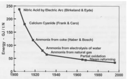
Figure 7. Historical changes in the energy requirement for N fertiliser production (Jenssen and Kongshaug, 2003).
The energy requirement has dramatically decreased over time from about 55 GJ/metric ton of ammonia produced in the 1950s to 35 GJ/ton in the 1970s, while nowadays the best plants using natural gas as feedstock need only 28 GJ/ton (Figure 7). The thermodynamic minimum energy requirement is 20 GJ/ton NH3 (Smil, 2001). Energy requirement for best technology in
practice using other raw material is presented in Table 4. Best available technology here refers to available commercial scale technique that can be implemented also considering economical constraints. According to the International Fertilizer Industry Association about 67% of global ammonia production is based on natural gas, 27% on coal while fuel oil and naphtha account for 5% (IFA, 2009a). Since a number of old plants are still in operation, the global average energy requirement was in 2008 around 37 GJ/ ton ammonia (ranging from 27-58 GJ/ton NH3) (IFA, 2009b).
Table 4. Comparison of best available process technology for ammonia production (IFA, 2009a)
Energy source Process Energy requirement
GJ/ton NH3 (GJ/ton NH3-N)
Natural gas Steam reforming 28 (34)
Naphtha Steam reforming 35 (43)
Heavy fuel oil Partial oxidation 38 (46)
Coal Partial oxidation 42 (51)
The GHG emissions associated with ammonia production are mainly CO2 in the flue gases
from the reforming and CO2 removal section, originating from the carbon in the fossil fuels
used. In partial oxidation plants, CO2 can also be emitted from power steam production in
2.5 Production of fertiliser products
Once ammonia is produced, it can be used to make straight nitrogen fertilisers or together with phosphate, potassium or micronutrients to make compound fertilisers (Figure 8).
Figure 8. Production route for commonly used fertilisers (EFMA, 2000). UAN=Urea Ammonium Nitrate (Solution), AN=Ammonium Nitrate, CAN= Calcium Ammonium Nitrate, NPK= Compound fertiliser containing Nitrogen, Phosphate and Potash.
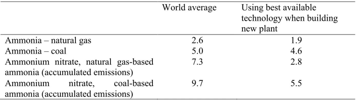
In this study, production of ammonium nitrate was investigated. To produce ammonium nitrate, about half the ammonia produced is first processed to nitric acid (the other half is used in the next step to produce ammonium nitrate solution). Nitric acid is produced by the exothermic reaction of ammonia and air over a catalyst and the absorption of the gas produced in water. By neutralising the nitric acid with the remainder of the ammonia, an ammonium nitrate solution is produced (exothermic reaction). The solution is then evaporated to remove water and the ammonium nitrate can be prilled or granulated to a final product. In the production of nitric acid, nitrous oxide (N2O), which is a strong GHG, is generated. In
recent years, catalytic filters have been installed in a number of plants to remove the nitrous oxides. This can greatly reduce the GHG emissions from ammonium nitrate production (Table 5).
Table 5. Greenhouse gas emissions from production of ammonia and ammonium nitrate (kg CO2-eq/kg N), based on IFA (2009a).
World average Using best available technology when building new plant
Ammonia – natural gas 2.6 1.9
Ammonia – coal 5.0 4.6
Ammonium nitrate, natural gas-based
ammonia (accumulated emissions) 7.3 2.8
Ammonium nitrate, coal-based ammonia (accumulated emissions)
9.7 5.5
2.6 Production of ammonia based on renewable energy
The hydrogen needed for ammonia synthesis can also be produced from renewable resources. There are four main options available for the production of renewable hydrogen for use in ammonia production (Chum and Overend, 2001; Ni et al., 2006):
1. Electrolysis based on renewable electricity. 2. Reforming of biogas.
3. Thermal conversion of biomass (pyrolysis and gasification).
4. Collection of hydrogen produced by algae and photosynthesising organisms. In this study, electrolysis (1) and thermal gasification (3) were studied.
Electrolysis is the process by which water is split into hydrogen and oxygen with the aid of electricity. Thermal gasification (partial oxidation) means that the biomass is combusted, but with a shortage of oxidant (air, oxygen and/or steam). Instead of producing heat as in normal combustion, the product is an energy-rich gas. The process is further described in Appendix A.
There have been some production facilities utilising electrolysis to produce hydrogen and then ammonia. In the 1940s and 1950s, several small-scale electrolytic ammonia plants were built in for example Norway, Egypt, Peru, Iceland and Zimbabwe. However, most of these have been decommissioned (UNIDO/IFDC, 1998). Between 1948 and 1990, the company Norsk Hydro operated a hydropower-driven electrolyser with 150 MW capacity, the hydrogen being used to produce ammonia. During the oil crisis in the 1970s and 1980s, production of ammonia on a small scale was considered as a way of reducing the dependency on fossil oil. Some studies were carried out on electrolysis-based ammonia production, see for example Dubey (1978), Jourdan and Roguenant, (1979) and Grundt and Christiansen (1982).
At present, the concept of small-scale renewable ammonia production is becoming interesting again, as a measure to reduce fossil fuel dependency and also reduce GHG emissions. In Minnesota, USA, a plant is currently being commissioned that will produce 1 ton per day ammonia from wind-powered electrolysis (New Energy and Fuel, 2010).
The concept of nitrogen fertilisers produced by reforming of biogas (2) and thermal gasification (3) has been studied by Ahlgren et al. (2008). However, collection of hydrogen produced by algae etc. (4) is very high-tech and the hydrogen production is so far only at laboratory-scale. As far as we know, the system has not been considered for ammonia production.
3 METHODS
3.1 Scenario construction
The aim of the present study was to evaluate the land use, energy use and GHG emissions from the production of ammonium nitrate based on renewable resources using life cycle assessment methodology.
However, a large part of the study consisted of describing reasonable technical solutions for the production of ‘green fertilisers’ and modelling the inputs and outputs in the processes. The description of the scenarios was prepared based on literature studies, but also on discussions with reference individuals associated with the project (see Acknowledgments). All modelling (processes, energy use, land use, GHG emissions, costs) was done in a spread sheet.
3.2 General introduction to life cycle assessment methodology
Life cycle assessment (LCA) is a methodology used for studying the potential impact on the environment caused by a chosen product, service or system. The product is followed through its entire life cycle. The amount of energy needed to produce the specific product and the environmental impact are calculated. The life cycle assessment is limited by its outer system boundaries (Figure 9). The energy and material flows across the boundaries are looked upon as inputs (resources) and outputs (emissions).
Figure 9. The life cycle model. Based on Baumann and Tillman (2004).
The methodology for conducting a life cycle assessment is standardised in ISO 14040 and 14044 series. According to this standard, a life cycle assessment consists of four phases (Figure 10). The first phase includes defining a goal and scope. This should include a description of why the LCA is being carried out, the boundaries of the system, the functional unit and the allocation procedure chosen. The second phase of an LCA is the inventory analysis, i.e. gathering of data and calculations to quantify inputs and outputs. The third phase is the impact assessment, where the data from the inventory analysis are related to specific environmental hazard parameters (for example CO2-equivalents). The fourth phase is
interpretation, where the aim is to analyse the results of the study, evaluate and reach conclusions and recommendations (ISO, 2006a, 2006b). In an LCA study, the phases are not carried out one by one but in an iterative process across the different phases.
R aw material acquisition
Waste management Processes Transports Manufacture U se R ESO U R C ES
e.g. raw materials, energy, land resources
EMISSIO N S to air, water, ground R aw material acquisition
Waste management Processes Transports Manufacture
U se R aw material acquisition
Waste management Processes Transports Manufacture U se R ESO U R C ES
e.g. raw materials, energy, land resources
EMISSIO N S to air, water, ground
Figure 10. Stages of an LCA (ISO, 2006a).
There are two main types of LCA studies; attributional and consequential. The attributional LCA study (sometimes also referred to as accounting type LCA) focuses on describing the flows to and from a studied life cycle. The consequential LCA (sometimes also referred to as change-orientated type LCA) focuses on describing how flows will change in response to possible decisions. Some authors state that attributional LCA are mainly used for existing systems, while consequential LCA are used for future changes (for example Baumann and Tillman, 2004). However as Finnveden et al. (2009) point out, both types of LCA can be used for evaluating past, current and future systems.
The type of LCA carried out has an impact on many of the methodological choices in an LCA. For example in handling of by-products, the attributional LCA uses an allocation based on mass, monetary value, etc. In a consequential LCA, a system expansion is instead often the choice, e.g. trying to determine the consequences of a new by-product appearing on the market. It also affects the choice of data; in a consequential LCA marginal data are used as it studies a change in a system, while an attributional LCA uses average data.
For LCA studies including use of biomass, the use of land must be included. When growing crops for energy purposes, land is needed. Quantifying emissions connected to loss or accumulation of carbon at the site of cultivation of the raw material can be referred to as the direct land use change.
In recent years, however, there have been calls to also include indirect land use. If the land used for energy crops was previously used for other activities, for example cereal production or pasture, it is probable that the demand for these products will still continue to exist. The demand for the products previously produced from the land now occupied by energy crops can be met by increasing the yields on the same land, or by moving the activities to another location. This moving of activities can cause land use changes, for example by utilisation of previously uncultivated land within the country under study or outside that country (Cherubini, 2010). However, quantification of indirect land use is very difficult and requires the use of economic equilibrium models and the results are associated with high uncertainty.
3.3 Chosen impact categories in the study
There are many impact categories that can be included in an LCA. In general, the categories can be divided into three main groups; resource use, human health and ecological consequences (Baumann and Tillman, 2004).
In this study, the resources categories studied were energy and land use. Energy analysis is often included as a step in the execution of a life cycle assessment, calculating the cumulative energy demand, often divided into renewable primary energy carriers (e.g. biomass) and
non-Goal and scope definition Inventory analysis Impact assessment Interpretation
renewable primary energy carriers (e.g. coal, oil, gas) (Jungmeier et al., 2003). The energy demand is often expressed as primary energy, which is defined as the energy extracted from the natural system before transformation to other energy carriers (Baumann & Tillman, 2004). In this study the energy use was expressed as primary fossil energy use. The primary energy factors are presented in Table 6.
Table 6. Primary energy factors used in the study
Diesel Natural gas Wind power (generated) Wind power (distributed) District heating (oil) Electricity (coal) 1.061 1.061 0.0472 0.0552 1.273 2.723
1Factor for production and distribution (Uppenberg et al., 2001).
2Factor for manufacture and decommissioning. Distributed means grid losses are included (Vattenfall, 2010). 3Including production, distribution and conversion losses (Uppenberg et al., 2001).
In the biomass scenarios, land is required for cultivation or collection of raw material. The land use is expressed as the number of hectares needed per functional unit (FU). However, it also important to account for any changes in the soil carbon content in the GHG balance. Therefore the former use of the land must be established. It is also important to establish whether any other land use activities have changed due to the raw material cultivation, for example whether a previous crop cultivation has been displaced to another location (indirect land use); this is dealt with in the sensitivity analyses.
The ecological consequence impact category investigated in this study was global warming potential. The characterisation factors were chosen for a 100-year perspective; fossil CO2: 1,
CH4: 25 and N2O: 298 (IPCC, 2007). The impact on human health was not assessed.
3.4 Functional unit in the study
In principle, all nitrogen fertilisers on the market today are based on fossil fuel. By producing nitrogen fertilisers based on renewable resources, the production of fossil fuel-based fertilisers can be avoided. The functional unit in this study was set to the production of 1 kg of fertiliser nitrogen based on renewable resources as ammonium nitrate (33.5% N) at the gate of the production facility, assuming that the nitrogen produced avoids the production of a fossil fuel-based alternative.
3.5 Overview of scenarios studied
Table 7 presents an overview of the five scenarios studied. In scenarios 1 and 2, wind power was assumed to be used to power an electrolysis process, producing the hydrogen needed for fertiliser production. Scenario 1 studied small-scale production, while scenario 2 studied large-scale production. In scenarios 3 and 4, combustion of biomass to produce heat and electricity was studied. In scenario 3 a new plant was assumed to be commissioned. Biomass then needs to be supplied from new land (this will give rise to land use change emissions, see further description in section 4.3). Scenario 4 assumed that the nitrogen fertiliser production is integrated into an existing CHP plant. The biomass used therefore does not need to be taken from new land. However, the electricity previously sold to the grid is now used for fertiliser production. This means that the electricity no longer put on the grid must be produced elsewhere (Figure 11). In scenario 5, a new plant utilising thermal gasification technology to produce hydrogen for fertiliser production was studied. In comparison with present
commercial-scale production sites, all scenarios studied can be considered small-scale. Thus the terms small-scale and large-scale production (Table 7) are used to distinguish differences in scale between the five scenarios and not in comparison with present production.
Table 7. Overview of scenarios 1 to 5
Scenario Scale Technology Short description
1 Small Wind power -
electrolysis - fertiliser production
New plant, wind power and fertiliser production at same location.
2 Large Wind power -
electrolysis - fertiliser production
New wind power connected to grid. New fertiliser plant can be located elsewhere, preferably close to end-user or harbour.
3 Large Combustion Salix/straw
- electrolysis - fertiliser production
New plant located close to raw material supply. Surplus heat used for district heating, replacing marginal heating.
4 Large Existing biomass CHP -
electrolysis - fertiliser production
Integrated fertiliser production in existing CHP (combustion of forest residues). The electricity no longer produced has to be replaced by production elsewhere. More heat than before integration will be produced, the extra heat replaces marginal alternative.
5 Large Thermochemical
gasification - fertiliser production
New plant located close to raw material supply. Electricity surplus sold to the grid, replacing marginal alternative.
The green fertilisers produced were assumed to outcompete other types of nitrogen (Figure 11). The question is what type of fertiliser is the green nitrogen replacing. This is important, since all CO2 savings are relative to this. This question is also vital for the heat and electricity
by-product credits.
Many LCA practitioners argue that when modelling a change, marginal data should be used, as it is the marginal production that is first affected by market changes (Ekvall and Weidema, 2004). In an energy use context this would typically be a fossil-based alternative. However this may not always be the case. As Finnveden (2008) points out, due to regulatory systems (such as the EU CO2 cap), the marginal might be a renewable fuel, or more likely a complex
mix of different types of energy sources. A number of energy prediction models are available to establish the marginal energy production, but it tends to be very difficult to model the effects in a proper way and the results are highly uncertain (Mathiesen et al., 2009). To highlight this uncertainty, Finnveden (2008) recommends that two scenarios be used in LCAs, one high CO2 emission marginal alternative and one with low CO2 emissions.
For the sake of simplicity, in this study we assumed that fossil oil is the marginal production for district heating and coal for electricity. For nitrogen fertilisers the marginal production was assumed to be an older natural gas plant without nitrous oxide removal. In the sensitivity analysis we investigated how the results are influenced by different assumptions of marginal production.
Figure 11. Visual description of calculation assumptions. In scenarios 3 and 5, it was assumed that raw material previously not harvested (straw) or planted on marginal land (Salix) is used. The products then replace marginal alternatives on the market. In scenario 4 it was assumed that the nitrogen production is integrated within an existing CHP (combined heat and power) plant. The electricity previously sold to the grid is then utilised for nitrogen production. This missing electricity on the market was assumed to be compensated for by marginal production. In scenario 4, only the excess heat compared with the existing CHP plant was accounted for.
3.6 System boundaries and delimitations
The emissions of GHG were quantified from ‘cradle-to-gate’, i.e. all the emissions stemming from raw material acquisition to ammonium nitrate product at the factory gate were included. The use of the fertiliser was therefore not included. However, in the biomass scenarios fertilisers are needed for cultivation. Therefore it was assumed that part of the ammonium nitrate produced is returned to the plantation/field. For Salix plantations, the amount of returned nitrogen was according to the fertiliser recommendations (Gustafsson et al., 2007), while for straw and forest residues the amount of returned nitrogen was calculated as the amount of nitrogen removed with the straw/residue (Phyllis, 2010). The emissions arising from the use of those fertilisers (mainly nitrous oxide from soil) were included in the calculations.
Furthermore, bottom ash from combustion and gasification, which contains valuable phosphorus and potassium, was assumed to be returned to the growing site. The return of ash to agricultural fields is not regulated by Swedish law. However, there are regulations for spreading of sewage sludge, which could serve as guidelines for upper limit of heavy metals (Gruvaeus and Marmolin, 2007).
In the electrolysis process, water is split to produce hydrogen. As a by-product, oxygen is formed. In the air separation unit used in the gasification scenarios to produce nitrogen,
Straw/Salix
Electricity Heat
Nitrogen fertiliser
Replaces marginal alternatives
Forest residues Electricity Heat Nitrogen fertiliser Marginal production Surplus compared to existing CHP replaces marginal alternative
Build a new plant (Scenario 3 and 5) Integrate in existing CHP (Scenario 4)
Replaces marginal alternative
+
Process Process Compensating for reduced electricity output from CHPoxygen is also formed as a by-product. The oxygen can be sold to other industries, but it is not certain that there is a market for this, so it was not given any value in this study.
Emissions from production of capital goods such as machinery and buildings were not included in the bioenergy calculations, since in previous studies they have been found to have little impact on the results when converting biomass to fuel (or, as in this case, to nitrogen) (Bernesson et al., 2004, 2006). In the wind power scenarios, however, the manufacturing and decommissioning were included.
3.7 Production costs
Production costs of AN fertilisers were calculated for two of the scenarios, scenarios 1 and 3. Electricity is used by all processes in the AN fertiliser production chain and was calculated separately in order to show the economic impact on total production costs from electricity generation. The costs for other processes in the AN production chain are shown excluding electricity costs.
Annual costs for producing AN fertiliser were estimated for fixed costs and costs for operation and maintenance (O&M). The base year for the economic calculations was set to 2010 and all costs collected from older sources were allocated to this year. An inflation calculator was used to recalculate US data to 2010 (Inflation calculator, 2011) using US consumer price indexes (CPI) for recalculation. Swedish costs were recalculated to 2010 using an inflation calculator from SCB (SCB, 2011). Costs in currencies other than SEK were first allocated to 2010, then yearly average currency data from Riksbanken (2011) were used to obtain cost in SEK from USD.
For electricity generation, the annual costs of the total investment cost (I) were calculated using the annuity method. The annuity method uses rate of interest (R) set to 6% and depreciation time (T) of 20 years to calculate the annuity factor (n) according to Equation 1:
Equation 1
The annuity factor (n) multiplied by total investment costs (I) gives the annual fixed costs (A) (Equation 2). Costs for O&M are calculated on an annual basis and then added to the annual fixed costs.
A=I*n Equation 2
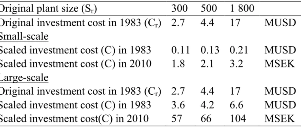
In the case of ammonia, nitric acid and AN fertiliser production, total annual costs (both fixed and O&M) for different plant sizes were taken from UNIDO (1983). These data were used instead of using the annuity method to calculate the electricity costs.
! ! !
In the case of small-scale production of ammonia, nitric acid and AN fertiliser, data for large-scale production were large-scaled down to fit small-large-scale production using cost and large-scale factors (Gerrard, 2000; Remer et al., 2008). The total cost of a proposed plant (C) with size (S) can be estimated from the total cost of a similar reference plant (Cr) with size (Sr) using Equation 3.
The scale exponent (n) can be derived from historical data for similar plants and is usually in the range 0.4-0.8, typically 0.65 (Gerrard, 2000).
Equation 3 ! !!! ! !! !
4 INVENTORY OF ENERGY AND EMISSION DATA
All data on emissions were taken from the literature. For a detailed description of the technical assumptions, see Appendix A and B.
4.1 Wind power
The emissions from wind power production arise in three phases: construction, operation and decommissioning (Tremeac and Meunier, 2009). A review of LCA studies on wind power was carried out by Varun et al. (2009). The GHG emissions varied between 9.7 and 39.4 g CO2-eq per kWh, with one study of small-scale wind power in Japan reporting 123.7 g CO2
-eq per kWh. In this study we chose to use data from an EPD (Environmental Product Declaration) carried out by Vattenfall (2010). The GHG emissions per kWh generated at the wind power plant are reported to be 15 g CO2-eq per kWh. The GHG emissions after
distribution assuming a 5% loss are 17 g CO2-eq per kWh.
In the small-scale wind power to nitrogen fertiliser system studied, the figure for generated electricity was assumed, while the distributed figure was used in the large-scale scenario.
4.2 Cultivation/collection of biomass raw material
The yield of straw was set to 4.3 ton dry matter per hectare and year. Data on the energy use for windrowing, baling and collection were taken from Nilsson (1997).
For Salix, a yield of 10 ton dry matter per hectare and year was assumed. Data on energy use for planting, weed control, harvest etc. were taken from Börjesson (2006).
For forest residues, it was assumed that 32 wet ton of residues per hectare are collected after final felling (RecAsh, 2009). This is an average yield after final felling of a mix of rich and poor spruce and pine stands. With a rotation time of 80 years, this on average gives 217 kg dry matter per hectare and year. Data on energy for collecting, bundling etc. were taken from Lindholm (2010).
4.3 Land use and soil carbon
4.3.1 Straw
In scenarios 3 and 5, straw was assumed to be used as raw material. Harvesting straw leads to no actual land use as it is a by-product from cereal cultivation. This is under the assumption that the straw is previously not utilised for any other purpose and therefore has no indirect effects on land use*.
However, harvesting straw can have an impact on the soil carbon content. The carbon no longer sequestered in the soil due to straw harvest has to be accounted for in the GHG balance. It is the difference on a long-term basis in soil carbon content between harvesting and not harvesting straw that should be counted. Straw incorporated into soil will decompose, but part will be transferred to the long-term soil carbon pool. The rate of decomposition
* There are no recent surveys of straw utilisation in Sweden, the latest one dating from 1997. In that, it was
estimated that 1% of the straw was burned on field, 64% incorporated in soil and 35% harvested (utilised as feed, litter and energy) (SCB, 1999). Here we assume that there is enough straw available for harvesting that is currently not utilised.
depends on many factors, such as the characteristics of the soil (e.g. structure, pH, initial carbon) and climate (e.g. temperature, humidity) and farming practices (e.g. rotation, tillage) (Johansson, 1994).
Trials with radioactive labelling in Sweden show that only 5-10% of incorporated carbon in straw is left in the soil after 10-20 years (Mattsson and Larsson, 2005). Assuming a straw harvest of 4 ton and a carbon content of 50% results in between 200 and 400 kg C left after 10-20 years. Assuming a longer time perspective would reduce the amount of carbon left. In a study by Johansson (1994), a model for soil carbon with and without straw removal showed a difference of 5300 kg C per hectare and year after 100 years (53 kg C difference per year on average). Based on long-term field results (Röing et al., 2005), we concluded that removal of straw has no impact on topsoil C. In yet another study modelling soil C removal, a variation of 78-385 kg C/ha and year was observed (Saffih-Hdadi and Mary, 2008).
In conclusion, the effect of straw harvest on soil C is difficult to assess and is dependent on local factors and the time period studied. In this study we assumed that removing straw results in a reduction of 150 kg C/ha and year, over a period of about 30–50 years after which the soil carbon level will have reached a new steady state (based on Börjesson and Tufvesson (2011)).
4.3.2 Salix
Salix was studied as raw material in scenarios 2 and 5. At present, only 15 000 ha of Salix are planted in Sweden. However, the potential is reported to be as large as 200 000 ha (SOU, 2007). In this study we assumed that the plantation of Salix will take place on land previously not used for other purposes. One good reason for this is that the land currently used for crops is most likely the best farm land. It would not be economically optimal to plant Salix on the best farm land, but rather on other types of land.
At present, about 5.8% (equal to 153 300 ha) of Swedish farm land is under fallow (SJV, 2008c). There is also a great deal of abandoned farm land, since the cultivated area has declined by about 300 000 hectares since the 1970s (SOU, 2007). According to a study by the Swedish Board of Agriculture, there is also an overproduction of 200 000-300 000 hectares of ley which is not utilised (SJV, 2008c). It is reasonable to believe that increased planting of Salix will take place on all these different types of land.
Planting Salix can have both negative and positive effects on soil carbon content. A combination of different previous land uses was assumed here (Table 8).
Table 8. Soil carbon increase when Salix is planted on different types of land and the assumed share of each land type converted
Fallow farm land (mineral soil) Fallow farm land (organic soil) Previously ley Abandoned farm land Soil carbon increase
(kg C/ha year) 5001 17002 01 03
Assumed share of land
used to plant Salix 50% 5% 20% 20%
1Ref: Börjesson (1999)
2Ref: Berglund and Berglund (2010)
3The quality of abandoned farm land varies a great deal, which makes it difficult to assess the effect of
cultivating Salix. We assumed that there is no increase in soil carbon.
The average soil carbon stock change for planting Salix in Sweden was calculated to be an average increase of 335 kg C/ha and year (1228 kg CO2-eq/ha and year) based on data in
Table 8. This is assumed over a period of about 30–50 years after which the soil carbon level will have reached a new steady state. Similar to straw removal, the uncertainty in carbon stock changes due to Salix plantation is very large and great variations are reported in the literature. Therefore this issue is further dealt with in the sensitivity analysis.
4.3.3 Forest residues
In scenario 4, forest residues are used as the raw material for nitrogen fertiliser production. Forest residues contain some carbon that would have been left in the forest if not utilised. In a study by Lindholm (2010), the effect on the soil carbon content when removing forest residues was analysed using a model and proved to be very dependent on the time frame assumed. Over a long time period (2-3 rotations or 240 years) the decrease in soil C was calculated to between 2.9 and 3.5 kg C/ha and year when removing logging residues after the final fellings. Other studies have found higher decreases, 17-50 kg C/ha and year (see review of other studies in Lindholm (2010)). In the present study an average loss of 3.2 kg soil C/ha and year was assumed in the base case scenario over a longer time period (2-3 rotations). This means that the time frame for soil carbon changes is different for the forest residue scenario compared to the straw and Salix scenarios. The reasoning behind this can be compared to the IPCC Guidelines where a stock change perspective is applied and the change in soil C is divided by a plantations life-time, IPCC has a default value of 20 years (IPCC, 2006). However, here we have used data for Salix and forest residues stretching out for two rotation periods. For straw, the rotation period argument can not be used, but we assumed same as for Salix since they both were assumed to effect farm land. There is no consensus on how soil carbon changes in bioenergy systems should be calculated over time (Lindholm, 2010), and the approach here applied can of course be discussed.
4.4 Transport of biomass raw material
The plants utilising biomass as raw material were assumed to be located in an area where there is a large resource available. The transport distance for biomass was calculated using the model described in Nilsson (1995) and Overend (1982). According to this, the area from which biomass is collected was assumed to be circular, with the plant in the centre. The
average transportation distance is dependent on the biomass requirements of the production plant, a road tortuosity factor and the available amount of biomass in the area.
4.5 Nitrogen fertiliser production
We studied two main routes for fertiliser production; via electrolysis of water and via thermal gasification (see Figure 2). Both of these processes aim to produce the hydrogen needed for ammonia synthesis, in which hydrogen and nitrogen from normal air are combined.
4.5.1 Hydrogen production via electrolysis
Four different electrolysis scenarios were studied, one small-scale (scenario 1) and three large-scale (scenarios 2, 3 and 4).
In the small-scale scenario, low temperature alkaline electrolysis was assumed and the electricity use set to 180 MJ per kg hydrogen (Zeng and Zhang, 2010). For large-scale production solid oxide high temperature electrolysis was assumed, utilising electricity (120 MJ/kg H2) and steam (28 MJ/kg H2), data collected from Zeng and Zhang (2010).
4.5.2 Hydrogen production via thermal gasification
For the thermochemical conversion route, only large-scale production was considered (scenario 5). The hydrogen yield and electricity requirement were based on data found in Hamelinck and Faaij (2002) and emissions data from Edwards et al. (2010).
4.5.3 Ammonia synthesis
For the large-scale scenarios, yields, energy consumption and steam production for ammonia synthesis were assumed to be similar to those of a natural gas-based system; data were taken from Dybkjær (2005) and Uhde (2011). The nitrogen required was assumed to be produced in a cryogenic air separation plant.
There are almost no small-scale ammonia facilities, not so much because of technical difficulties but due to economies of scale. A small-scale facility cannot invest in turbines and can therefore not fully utilise the high pressure steam formed in different parts of the process. Instead pumps, compressors etc. must be driven by electricity (UNIDO/IFDC, 1998; Noelker, 2010). Nitrogen was assumed to be produced by pressure swing adsorption and a De-oxo unit. An energy requirement of 3.3 MJ/kg NH3 was assumed for the ammonia production step (for
air separation, compression, ammonia synthesis loop etc) (see further description in Appendix A).
4.5.4 Nitric acid production
Nitric acid is produced by the exothermic reaction of ammonia and air over a catalyst and the absorption of the product gas in water. Data for yields, electricity use and steam production were taken from IPPC (2007) and Saigne (1993). One can suspect that there will be larger heat losses per mass unit in a small scale system. However, due to lack of data, no distinction was made between large- and small-scale production. It was however assumed that in the small scale process, non of the steam could be utilised for electricity generation.
In the reaction, nitrous oxides (N2O) are generated. However, using a combination of
abatement techniques, the N2O emissions from a modern new built plant can be limited to
between 0.12 and 0.6 kg N2O/ton nitric acid (100%) according to IPPC (2007). Here we
assumed 0.6 kg/ton nitric acid (100%) in all scenarios, which recalculated can be expressed as 2.8 g N2O/kg N. Due to lack of data, no distinction was made between large- and small-scale
4.5.5 Ammonium nitrate production
By neutralising the nitric acid with the remainder of the ammonia, an ammonium nitrate solution is produced (exothermic reaction). The solution is evaporated to remove water. A modern plant produces enough heat in the neutralisation to remove the water and no additional heat is needed (Jenssen and Kongshaug, 2003). The ammonium nitrate is thereafter granulated. The electricity requirement is relatively small, 25 kWh/ton ammonium nitrate produced (EFMA, 2000). Due to lack of data, no distinction was made between large- and small-scale production.
4.6 Energy credit/debt
In some scenarios there will be a surplus of heat and/or electricity. In the scenario where nitrogen production is integrated into an existing CHP, the electricity previously sold to the electric grid will be used for the electrolysis process and the missing electricity will need to be produced elsewhere. In this study we assumed that fossil oil is the marginal production for district heating and coal for electricity (emissions data taken from Uppenberg et al., 2001).
4.7 Replaced fossil nitrogen fertiliser
For nitrogen fertilisers the marginal production was assumed to be an older natural gas plant without nitrous oxide removal, with emissions of 7.3 kg CO2-eq/kg N equivalent to the world
5 INPUT DATA FOR ESTIMATION OF PRODUCTION COSTS
All data on costs were taken from the literature. For a description of the technical assumptions, see the preceding section and Appendix A.
5.1 Wind power
Using data from Hansson et al. (2007) and Wizelius (2009), the costs for producing land-based wind power in Sweden can be calculated (Table 9). Fixed costs are calculated for 20 years depreciation time with 6% interest. This equals an electricity production cost of 310 SEK per MWh. Annual average spot price of electricity in 2010 was 506 SEK per MWh (Nord Pool, 2011).
Table 9. Yearly fixed and running costs for a wind power unit with an effect of 2 MW
Costs Unit
Annual investment cost 559 SEK/MWhel
Costs for operation and maintenance 51 SEK/MWhel
Green certificate -295 SEK/MWhel
Total costs 315 SEK/MWhel
5.2 Power generation in CHP
In the case of large-scale production of ammonia, biomass is combusted in a CHP plant. Electricity and steam are used in all processes from electrolysis, ammonia and nitric acid production and for producing AN fertilisers. The accumulated daily electricity requirement is 1 400 MWh. This equals a CHP plant producing 78 MW of electricity and 195 MW heat. The plant uses 1 314 GWh of fuel per annum. Assuming biomass with a lower heat value (LHV) of 5.14 MWh per ton, 256 000 metric tons of biomass are used as fuel every year.
Dimensioning full load hours for CHP was set to 7 000 hours per year. This is somewhat higher than data from Nyström et al. (2011), which used 5 000 hours per year. CHP is usually dimensioned for supplying district heating during season, hence the low amount of full load hours. In the current study it was assumed that the plant is run in order to utilise fuel more effectively as in polygeneration.
Costs for producing electricity in the CHP plant were taken from Nyström et al. (2011). The heat was given a credit of 232 SEK/MWhth. It was also assumed that the production will be
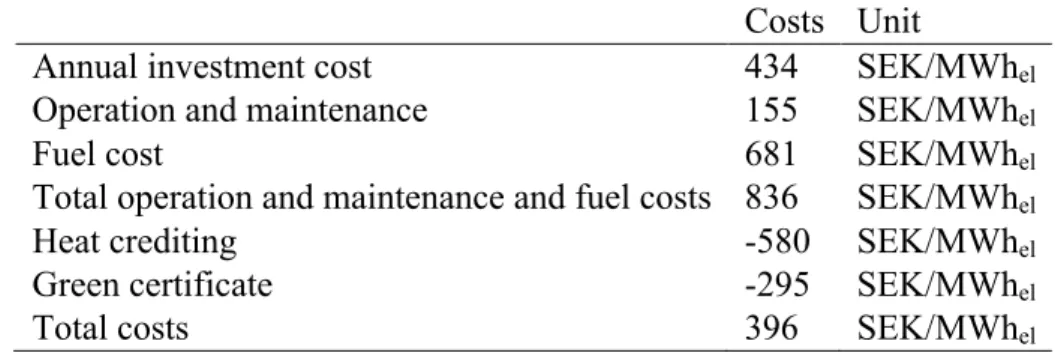
given green electricity certificates with a value of 295 SEK/MWh electricity. The biomass fuel cost was set to 210 SEK/MWh LHV. The total electricity production costs when considering certificate and heat crediting were 396 SEK per MWh electricity produced (Table 10).
Table 10. Yearly fixed and operational costs for biomass-fuelled CHP
Costs Unit
Annual investment cost 434 SEK/MWhel
Operation and maintenance 155 SEK/MWhel
Fuel cost 681 SEK/MWhel
Total operation and maintenance and fuel costs 836 SEK/MWhel
Heat crediting -580 SEK/MWhel
Green certificate -295 SEK/MWhel
Total costs 396 SEK/MWhel
5.3 Electrolysis and hydrogen storage
The cost of producing hydrogen in a small scale electrolysis unit was based on data in Saur (2008). Depending on currency rates and year of calculation, the cost of producing hydrogen through electrolysis ranges between 2.5-12 USD per kg H2 according to Saur (2008). This
equals 15-87 SEK per kg H2 in 2010, excluding electricity costs (Table 11). The cost of an
electrolyser unit producing 181 kg H2 per day (the minimum hydrogen needed for producing
1 ton of NH3) was calculated to be 34 SEK per kg H2 or 2.3 MSEK per year.
Table 11. Costs for an electrolysis plant producing 100 and 1 000 kg H2 per day (Saur, 2008) and the
calculated costs for producing 182 kg H2 per day
Size, installation 100 182 1 000 Unit Ref Saur, 2008 Calculated Saur, 2008
Capital cost 26 25 11 SEK/kg H2
Fixed O&M 10 9 4 SEK/kg H2
Total costs 36 34 15 SEK/kg H2
There is a need to store hydrogen for buffering against uneven wind conditions. Generated electricity is fed directly into the process and it was assumed here that no surplus electricity is generated. Costs for storing hydrogen were calculated for the amounts of hydrogen needed for 5 days production of ammonia. Hydrogen was assumed to be stored aboveground, compressed at 350 bar pressure.
The cost for hydrogen storage is a function of amount of hydrogen stored and time of storage. These costs were calculated using data from Amos (1998) and varied between 6.6-15.6 SEK per kg H2 stored.
For large-scale hydrogen production, data from data from Hulteberg and Karlsson (2009) was used. A cost of 7 SEK per kg H2 for large-scale electrolysis excluding electricity costs was
calculated from Hulteberg and Karlsson (2009) for a plant producing 15 000 ton H2 per year.
This also excludes contingency and contracting costs. According to data from Hulteberg and Karlsson (2009) the hydrogen production cost would be roughly 10 SEK/kg H2 if contingency
and contracting costs were included and around 40 SEK/kg H2 if the electricity cost also was
included. The calculation was assumed valid for our modelled unit producing 38 ton hydrogen per day, this being the minimum amount of hydrogen required in order to produce ammonia sufficient for the requirements of the large-scale scenario.