ANALYTICAL SOLUTION FOR ANOMALOUS DIFFUSION IN FRACTURED NANO-POROUS RESERVOIRS
by Ali Albinali
Copyright by Ali A. Albinali 2016
ii
A dissertation submitted to the Faculty and the Board of Trustees of the Colorado School of Mines in partial fulfillment of the requirements for the degree of Doctor of Philosophy (Petroleum Engineering). Golden, Colorado Date Signed: Ali Albinali Signed: Dr. Erdal Ozkan Professor and Head Dissertation Advisor
Golden, Colorado
Date
Signed:
Dr. Erdal Ozkan Professor and Head Department of Petroleum Engineering
iii
ABSTRACT
This dissertation presents an analytical fluid flow model for multi-fractured horizontal wells in unconventional naturally fractured reservoirs. The solution builds on anomalous diffusion concept and fractional calculus to account for non-uniform velocity in highly disordered porous media. The mathematical model is derived for an isothermal, single phase and slightly compressible fluid. The model computes the transient bottomhole pressure solution for the well and is referred to as Tri-Linear Anomalous Diffusion and Dual-Porosity (TADDP) model.
In this work, a time-dependent flux incorporating the fractional derivative of the process variable is utilized and combined with the classical mass balance equation. The temporal derivative power is used to describe the heterogeneity of the flow field. Fractional calculus allows accounting for non-localities of flow and the heterogeneity caused by the contrast between the properties of the rock matrix and natural fractures. The anomalous diffusion formulation is applied to the tri-linear model (TLM) by Ozkan et al. (2009) where the dual-porosity idealization is utilized to describe the naturally fractured reservoir between hydraulic fractures (the so-called stimulated reservoir volume, SRV) and fluid transfer takes place i) from tight rock matrix to natural fractures, ii) from natural fractures to the hydraulic fractures and iii) from hydraulic fractures to the wellbore. The option to use the conventional Darcy’s law for the flux is also available.
Flow is treated independently in the rock matrix and natural fractures. In these domains, transport can be modeled by anomalous diffusion or normal diffusion. This approach provides flexibility in modeling natural fractures of discrete or sparse nature as well as modeling complex flow field in the matrix due to the presence of organic and inorganic content.
Results show that the solution concurs with the established models and adheres to the general physics of fluid flow. The effects of anomalous diffusion at different reservoir regions can be interpreted from pressure data and delays in the flow can be addressed by adjusting the diffusion exponent. The model offers a range of answers compared to the conventional dual-porosity models and provides utility to model various flow heterogeneities and reservoir types.
iv
TABLE OF CONTENTS
ABSTRACT ... iii
LIST OF FIGURES ... viii
LIST OF TABLES ... x LIST OF EQUATIONS ... xi ACKNOWLEDGMENTS ... xxiv DEDICATION ... xxv CHAPTER 1 INTRODUCTION ... 1 1.1 Problem Statement ... 1 1.2 Motivation ... 6 1.3 Hypotheses ... 8 1.4 Objectives ... 8 1.5 Methodology ... 9
1.6 Organization of the Dissertation ... 10
CHAPTER 2 LITERATURE REVIEW ... 11
2.1 Dual-porosity Models ... 12
v
2.3 Discrete Fracture Network Models ... 14
2.4 Fractals ... 15
2.5 Anomalous Diffusion ... 18
2.6 Notable Models ... 20
CHAPTER 3 ANALYTICAL MODEL... 23
3.1 The Flux Law ... 23
3.2 General Approach, Assumptions, and Definitions ... 25
3.3 Overview of the Tri-Linear Flow Model ... 27
3.4 Flow in the Outer Reservoir ... 29
3.5 Flow in the Inner Reservoir ... 30
3.5.1 Flow in the Matrix Elements... 30
3.5.2 Flow in the Natural Fractures Network ... 31
3.6 Flow in the Hydraulic Fracture ... 33
3.7 Matrix Elements of Different Properties... 34
CHAPTER 4 VERIFICATION AND ANALYSIS ... 36
4.1 Verification Under Normal Diffusion ... 36
vi
4.1.2 Dual-Porosity Idealization ... 37
4.2 Verification for Anomalous Diffusion ... 39
4.2.1 TLM with Anomalous Diffusion and Single-Porosity Inner Reservoir ... 39
4.2.2 Numerical 1D, Single-Porosity Solution ... 40
4.2.3 Analytical 1D, Single-Porosity Solution... 42
4.3 Sensitivity Analysis and Discussion of Results ... 42
4.3.1 Diffusion Exponent ... 42
4.3.2 Regional Impact ... 45
4.3.3 Flow Capacity ... 46
4.4 Field Application ... 47
4.4.1 Eagle Ford Shale ... 48
4.4.2 Niobrara Shale ... 50
CHAPTER 5 CONCLUSIONS AND RECOMMENDATIONS ... 54
5.1 Conclusions ... 54
vii
NOMENCLATURE ... 56
REFERENCES ... 58
APPENDIX A DERIVATION OF THE TADDP MODEL ... 63
A.1 Solution Derivation ... 63
A.2 The Outer Reservoir ... 65
A.3 The Inner Reservoir ... 67
A.3.1 The Matrix Elements... 68
A.3.2 The Natural Fractures ... 70
viii
LIST OF FIGURES
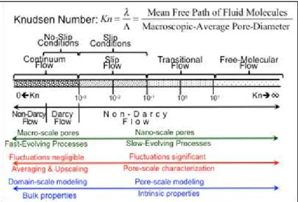
Figure 1.1: Knudsen Number and Flow Mechanisms (Roy et al. 2003). ... 3
Figure 1.2: The Koch Curve (Ben-Avraham and Havlin 2000). ... 6
Figure 1.3: Examples of Generated Fractal Networks (Acuna and Yortsos 1995). ... 7
Figure 2.1: Dual-Porosity Idealization (Kuchuk and Biryukov 2013). ... 13
Figure 2.2: Examples of Deterministic and Stochastic DFN Models (Dershowitz and Einstein 1988). ... 14
Figure 2.3: Idealization of Triple-Porosity Systems (Abdassah and Ershaghi 1986). ... 20
Figure 3.1: Illustration of the Symmetry Element and DP Idealization used in the Model. ... 26
Figure 3.2: The Tri-Linear Model (Ozkan et al. 2009). ... 28
Figure 4.1: Verification for Homogeneous Reservoir. ... 38
Figure 4.2: Verification for Dual-Porosity Assumption. ... 38
Figure 4.3: Verification for Anomalous Diffusion for Single-porosity Inner Reservoir. ... 40
Figure 4.4: Verification with Numerical 1D Anomalous Diffusion. ... 41
Figure 4.5: Comparison with Analytical 1D Solution. ... 43
Figure 4.6: Natural-Fracture Diffusion Exponent Sensitivity... 45
Figure 4.7: Matrix Diffusion Exponent Sensitivity. ... 45
ix
Figure 4.9: Regional Impact of Diffusion Exponent. ... 47
Figure 4.10: Analysis on Flow Capacity in Natural Fractures... 48
Figure 4.11: Analysis on Flow Capacity in the Matrix. ... 48
Figure 4.12: TADDP-Eagle Ford Match. ... 51
Figure 4.13: TADDP-Niobrara Match. ... 53
Figure A.1: Illustration of the Symmetry Element and DP Idealization used in the Model. ... 63
x
LIST OF TABLES
Table 4.1: Data Used for Normal Diffusion Verification. ... 37
Table 4.2: Dual-porosity Parameters Used in §4.1.2. ... 39
Table 4.3: Data Used in §4.2.2 and §4.2.3. ... 41
Table 4.4: Data Used for the Analysis of Results and Sensitivity Study. ... 44
Table 4.5: Match Parameter by Curnow (2015) DPDK Model. ... 50
Table 4.6: TADDP-Eagle Ford Match Input Data. ... 51
Table 4.7: Niobrara Shale Data. ... 52
Table 4.8: TADDP-Niobrara Match Input Data. ... 53
xi LIST OF EQUATIONS Equation (1.1). ... 3 Equation (1.2). ... 3 Equation (1.3). ... 5 Equation (1.4). ... 6 Equation (2.1). ... 12 Equation (2.2). ... 15 Equation (2.3). ... 15 Equation (2.4). ... 16 Equation (2.5). ... 16 Equation (2.6). ... 17 Equation (2.7). ... 17 Equation (2.8). ... 18 Equation (2.9). ... 18 Equation (2.10). ... 18 Equation (2.11). ... 18 Equation (2.12). ... 19
xii Equation (2.13). ... 19 Equation (2.14). ... 19 Equation (3.1). ... 23 Equation (3.2). ... 24 Equation (3.3). ... 24 Equation (3.4). ... 24 Equation (3.5). ... 27 Equation (3.6). ... 27 Equation (3.7). ... 27 Equation (3.8). ... 27 Equation (3.9). ... 27 Equation (3.10). ... 27 Equation (3.11). ... 27 Equation (3.12). ... 27 Equation (3.13). ... 27 Equation (3.14). ... 29 Equation (3.15). ... 29
xiii Equation (3.16). ... 29 Equation (3.17). ... 30 Equation (3.18). ... 30 Equation (3.19). ... 30 Equation (3.20). ... 30 Equation (3.21). ... 30 Equation (3.22). ... 31 Equation (3.23). ... 31 Equation (3.24). ... 31 Equation (3.25). ... 31 Equation (3.26). ... 31 Equation (3.27). ... 31 Equation (3.28). ... 31 Equation (3.29). ... 32 Equation (3.30). ... 32 Equation (3.31). ... 32 Equation (3.32). ... 32
xiv Equation (3.33). ... 32 Equation (3.34). ... 33 Equation (3.35). ... 33 Equation (3.36). ... 33 Equation (3.37). ... 33 Equation (3.38). ... 33 Equation (3.39). ... 33 Equation (3.40). ... 33 Equation (3.41). ... 34 Equation (3.42). ... 34 Equation (3.43). ... 34 Equation (3.44). ... 34 Equation (3.45). ... 34 Equation (3.46). ... 34 Equation (3.47). ... 35 Equation (3.48). ... 35 Equation (3.49). ... 35
xv Equation (A.1.1)... 64 Equation (A.1.2)... 64 Equation (A.1.3)... 64 Equation (A.1.4)... 64 Equation (A.1.5)... 64 Equation (A.1.6)... 64 Equation (A.1.7)... 64 Equation (A.1.8)... 64 Equation (A.1.9)... 64 Equation (A.2.1)... 65 Equation (A.2.2)... 65 Equation (A.2.3)... 65 Equation (A.2.4)... 66 Equation (A.2.5)... 66 Equation (A.2.6)... 66 Equation (A.2.7)... 66 Equation (A.2.8)... 66
xvi Equation (A.2.9)... 66 Equation (A.2.10)... 66 Equation (A.2.11)... 66 Equation (A.2.12)... 66 Equation (A.2.13)... 67 Equation (A.2.14)... 67 Equation (A.2.15)... 67 Equation (A.2.16)... 67 Equation (A.2.17)... 67 Equation (A.2.18)... 67 Equation (A.2.19)... 67 Equation (A.3.1.1)... 68 Equation (A.3.1.2)... 68 Equation (A.3.1.3)... 68 Equation (A.3.1.4)... 68 Equation (A.3.1.5)... 68 Equation (A.3.1.6)... 68
xvii Equation (A.3.1.7)... 68 Equation (A.3.1.8)... 68 Equation (A.3.1.9)... 69 Equation (A.3.1.10)... 69 Equation (A.3.1.11)... 69 Equation (A.3.1.12)... 69 Equation (A.3.1.13)... 69 Equation (A.3.1.14)... 69 Equation (A.3.1.15)... 69 Equation (A.3.1.16)... 69 Equation (A.3.1.17)... 69 Equation (A.3.1.18)... 70 Equation (A.3.1.19)... 70 Equation (A.3.1.20)... 70 Equation (A.3.1.21)... 70 Equation (A.3.1.22)... 70 Equation (A.3.2.1)... 70
xviii Equation (A.3.2.2)... 70 Equation (A.3.2.3)... 70 Equation (A.3.2.4)... 71 Equation (A.3.2.5)... 71 Equation (A.3.2.6)... 71 Equation (A.3.2.7)... 71 Equation (A.3.2.8)... 71 Equation (A.3.2.9)... 71 Equation (A.3.2.10)... 71 Equation (A.3.2.11)... 71 Equation (A.3.2.12)... 72 Equation (A.3.2.13)... 72 Equation (A.3.2.14)... 72 Equation (A.3.2.15)... 72 Equation (A.3.2.16)... 72 Equation (A.3.2.17)... 72 Equation (A.3.2.18)... 72
xix Equation (A.3.2.19)... 72 Equation (A.3.2.20)... 73 Equation (A.3.2.21)... 73 Equation (A.3.2.22)... 73 Equation (A.3.2.23)... 73 Equation (A.3.2.24)... 73 Equation (A.3.2.25)... 73 Equation (A.3.2.26)... 73 Equation (A.3.2.27)... 74 Equation (A.3.2.28)... 74 Equation (A.3.2.29)... 74 Equation (A.3.2.30)... 74 Equation (A.3.2.31)... 74 Equation (A.3.2.32)... 74 Equation (A.3.2.33)... 74 Equation (A.3.2.34)... 75 Equation (A.3.2.35)... 75
xx Equation (A.3.2.36)... 75 Equation (A.3.2.37)... 75 Equation (A.3.2.38)... 75 Equation (A.3.2.39)... 75 Equation (A.3.2.40)... 75 Equation (A.3.2.41)... 76 Equation (A.3.2.42)... 76 Equation (A.3.2.43)... 76 Equation (A.3.2.44)... 76 Equation (A.3.2.45)... 76 Equation (A.3.2.46)... 76 Equation (A.3.2.47)... 76 Equation (A.3.2.48)... 76 Equation (A.3.2.49)... 77 Equation (A.3.2.50)... 77 Equation (A.4.1)... 77 Equation (A.4.2)... 77
xxi Equation (A.4.3)... 77 Equation (A.4.4)... 77 Equation (A.4.5)... 77 Equation (A.4.6)... 78 Equation (A.4.7)... 78 Equation (A.4.8)... 78 Equation (A.4.9)... 78 Equation (A.4.10)... 78 Equation (A.4.11)... 78 Equation (A.4.12)... 78 Equation (A.4.13)... 78 Equation (A.4.14)... 79 Equation (A.4.15)... 79 Equation (A.4.16)... 79 Equation (A.4.17)... 79 Equation (A.4.18)... 79 Equation (A.4.19)... 79
xxii Equation (A.4.20)... 79 Equation (A.4.21)... 79 Equation (A.4.22)... 80 Equation (A.4.23)... 80 Equation (A.4.24)... 80 Equation (A.4.25)... 80 Equation (A.4.26)... 80 Equation (A.4.27)... 80 Equation (A.4.28)... 80 Equation (A.4.29)... 80 Equation (A.4.30)... 80 Equation (A.4.31)... 81 Equation (A.4.32)... 81 Equation (A.4.33)... 81 Equation (A.4.34)... 81 Equation (A.4.35)... 81 Equation (A.4.36)... 81
xxiii Equation (A.4.37)... 81 Equation (A.4.38)... 81 Equation (A.4.39)... 81 Equation (A.4.40)... 81 Equation (A.4.41)... 82 Equation (A.4.42)... 82 Equation (A.4.43)... 82 Equation (A.4.44)... 82 Equation (A.4.45)... 82 Equation (A.4.46)... 82 Equation (A.4.47)... 82 Equation (A.4.48)... 82 Equation (A.4.49)... 82
xxiv
ACKNOWLEDGMENTS
I would like to thank Saudi Aramco for supporting my education and providing the scholarship for my Doctorate degree. I would like to thank my advisor Dr. Erdal Ozkan for his supervision and help throughout my graduate studies at Colorado School of Mines. Dr. Ozkan taught me how to solve reservoir-engineering problems using analytical techniques and was very generous and patient guiding me to complete this dissertation. I also would like to thank Dr. Azra Tutuncu for her support and kindness. I would like to thank Dr. Carol Dahl for sharing her experience and guiding me through energy economics. I would like to thank committee members, Dr. Ugur Ozbay and Dr. Xiaolong Yin, for discussions and participation in my research. I also would like to thank all the professors at the Petroleum Engineering Department. Special thanks to the administrative PE staff, Denise Winn-Bower and Terri Snyder.
I would like to thank my family for their support and I extend my sincere gratitude and appreciation to my beloved mother for her prayers, love and support.
xxv
DEDICATION
This dissertation is dedicated to my dear mother who has been loving and taking care of me for all of my life. It is impossible to thank you adequately.
1
CHAPTER 1
INTRODUCTION
This dissertation presents the results of the research project for the degree of Doctor of Philosophy conducted under the Unconventional Reservoir Engineering Project (UREP) in the Petroleum Engineering Department at Colorado School of Mines. The objective of this research is to utilize the concept of anomalous diffusion and fractional calculus to provide an alternative modeling approach to the conventional mathematical models of reservoir engineering.
An analytical solution has been developed in this PhD research to model fluid flow in naturally fractured unconventional reservoirs by adopting the concept of anomalous diffusion (AD). The model utilizes the premise that micro-fractures of various scales are distributed heterogeneously and connected at various degrees to enhance fluid flow and communicate with hydraulic fractures to deliver fluids to the wellbore. The heterogeneity of the system can be described by adjusting the diffusion exponent 1 ≤ α < 0, where α = 1 corresponds to normal diffusion (ND) or a system with normally distributed properties and as α decreases the flow deviates from normal diffusion.
The remainder of this chapter discusses the problem statement, motivation, hypotheses, objectives, methodology of the research, and organization of the dissertation.
1.1 Problem Statement
More than half of the world’s hydrocarbon resources are in naturally fractured reservoirs (NFRs). Inherently, flow in NFRs is a complex phenomenon and poses profound challenges if attempted to be modeled in full complexity. Chronologically, fractured reservoirs have been modeled as homogenous media with enhanced permeability, dual-porosity (DP) media where matrix is represented as a distributed source feeding into the low-storativity but high-conductivity fracture medium, homogeneous matrix with a discrete fracture network, and as a fractal reservoir. Each of these approaches may be preferred for different reasons, but fundamentally, they all present an approximation to flow in naturally fractured reservoirs.
2
Recently, the industry’s focus on fractured unconventional reservoirs has increased and the models used for NFRs have come under greater scrutiny (Kuchuk and Biryukov 2013). Due to the more common use of the dual-porosity and discrete fracture networks models, most discussions are on the appropriateness of these models in general or under specific conditions. The objective of this research is to provide an account of anomalous-diffusion models for naturally fractured reservoirs in comparison to the dual-porosity idealization with a focus on nano-porosity unconventional reservoirs. In addition to the existing fractal reservoir and anomalous diffusion models, a new model will be derived, verified, and tested with production data from unconventional reservoirs.
Pores in unconventional reservoirs range in radii from a few to hundreds of nano-meters. In this environment, the continuum approach breaks down and different flow mechanisms dominate the mass transport. For example, considering gas flow, it is expected that the collisions between moving fluid particles become less often than collision with the walls of the flow channel as the apertures of flow channels approach nanometers (Ozkan 2013). One parameter that is used to characterize the flow is the Knudsen number (Kn), which is the ratio of the
molecular mean free path to the system’s representative physical length scale. Figure 1.1 in page 3 illustrates the expected flow behavior as a function of Knudsen number. The continuum approach is invalid at larger Knudsen numbers, which occur in environments of small characteristic length or low gas density. In addition, heterogeneity in unconventional reservoirs can create differences in fluid composition and pressure profile, which adds to the complexity when trying to understand the processes and interactions of controlling parameters. Yet, most of the fluid flow models depend on the conventional approach, which assumes either uniform or continuous reservoir properties and do not account for the deviations from our conventional perceptions.
Two issues need to be mentioned about the conventional understanding of fluid flow in porous media. First, it relies on spatially averaged properties (pressure, permeability, porosity, saturation, etc.) and the porous medium is assumed to form a continuum. Constitutive laws and conservation equations that are consistent with this perception describe fluid flow. Second, the conventional mathematical models follow the normal diffusion process (also called standard, classical or linear diffusion), which is suitable for systems where particles migrate randomly
3
under a Gaussian type distribution function with the probability to transition from the current location to the next governed by the current conditions. Time steps as well as distance travelled are discrete and equal for every migration and the probabilities to travel to the next-nearest sites are equal and sum to unity. Thus, the assumptions and simplifications underneath normal diffusion lead to the conclusion that the flow of fluid between two points is independent of history; that is, flow is instantaneous and governed by the current potential applied between the two points. Normal diffusion suggests that a particle’s mean square root of displacement r is related to time t by
. (1.1)
The normal diffusion equation that governs conventional fluid flow models is written as
, (1.2)
where D is the diffusion coefficient of the medium.
Figure 1.1: Knudsen Number and Flow Mechanisms (Roy et al. 2003).
The most commonly used models to describe fluid flow in NFRs are the dual-porosity/single-permeability models, often referred to as DP models. The formulation was first introduced by Barenblatt et al. (1960) who assumed pseudo-steady state flow from matrix to
4
fractures without including any details of the flow in the matrix medium. The model assumes immediate replacement of the volume produced from the fractures by the fluid contributed by the matrix. Later variations extended the model to multi-dimensional problems and additional features such as transient flow in the matrix and multiphase flow.
The DP approach relies on the premise that matrix provides the storage capacity and fractures provide the conductive paths. Conventional DP models account for advective flow only (Darcy flow) in the matrix and fractures. This approach, in essence, translates reservoir into an equivalent homogenous medium made out of effective (volume averaged) fracture properties and accounts for the flow from the matrix as an additional source term for the fracture medium. In addition, analytical DP models assume uniform matrix and fracture properties across the reservoir.
Data collected from well logging and outcrops suggest that a considerable variation of properties exist in unconventional NFRs; connected and isolated pores, discrete and continuous fractures with different characteristics and changing hydrocarbons properties (Camacho-Velázquez et al. 2012). Thus, the structure of unconventional porous media is better characterized with properties of different spatial scale, such as length, width, orientation, conductivity, etc., to account for these geological and petrophysical complexities. The arrangement of these features will affect the flow regimes as discussed by Kuchuk and Biryukov (2013) where a flow regime could be elongated, early terminated or masked by another regime. Hence, inhomogeneous scale of properties plays a major rule in the transport process and can impose complex flow events and fluid transport in fractured media with complex geometry is similar to anomalous diffusion in disordered media.
Several mathematical assumptions can lead to anomalous diffusion formulation. These assumptions range from diffusion following a power-law as a function of distance, fluid particles following a Continuous-Time-Random-Walk (CTRW) behavior, or different observation and correlation scales (Raghavan 2011). Due to the heterogeneous structure of porous media, diffusion can be faster or slower than normal diffusion. Thus, the application of anomalous diffusion becomes useful in replicating fluid flow in unconventional reservoirs, specifically where sharp contrasts exist between the scales of pores. In the context of tight, fractured
5
unconventional reservoirs, non-local anomalous diffusion arises in nano-porous matrix since the global pressure, which is governed by advective flow in fractures, influences local gradients of the mean diffusion process in the matrix. Thus, the resulting non-local anomalous diffusion equation is scale and memory dependent (Ozkan 2013). Anomalous diffusion relates the mean-square displacement of a particle to time by the following relation:
, where γ = 1 Normal diffusion. (1.3) γ ≠ 1 Anomalous diffusion. γ > 1 Super-diffusion. γ < 1 Sub-diffusion.
Several forms have been derived and provided as solutions for fluid flow in porous media with fractal properties in the literature (e.g., O’Shaugnessy and Procaccia 1985, Chang and Yortsos 1990, Acuna and Yortsos 1995, Flamenco-Lopez and Camacho-Velázquez 2003, Fuentes-Cruz et al. 2010, Cossio et al. 2012). In addition, several researchers have incorporated some of the specific features pertaining to hydrocarbon reservoirs and producing wells, such as naturally fractured reservoirs and hydraulically fractured wells. Some of these models will be reviewed in the literature review chapter.
The concept of fractal geometries allows development of practical models describing a medium with disordered properties. Fractals are generated using repetitive patterns and can be described mathematically using certain algorithms. Looking at fractal bodies, one would find that the attributes of any part of the structure are similar to the whole. When constructing fractals there is an initiator and generators. After each generation step i, N number of generators replace the initiator. For example, in Figure 1.2, panel-a is the original initiator or the first segment built (a straight line). The first generation is shown in panel-b where four equal segments replace the original line and the generated bodies are downscaled in size by one third of the initiator. Panel-c shows the second generation where every segment from the previous, or the first, generation is considered an initiator and is replaced by four generators.
6
a) Initiator b) 1st Generation c) 2nd Generation
Figure 1.2: The Koch Curve (Ben-Avraham and Havlin 2000).
The produced segments look like the initiator; they are straight lines, but the size is reduced. For the presented Koch curve, the reduction in size b-1 is one third. This leads us to the definition of the fractal dimension df, which is considered as a self-similarity dimension and
defined as
. (1.4)
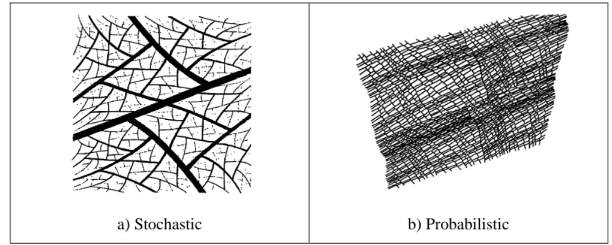
Thus, the fractal dimension of the Koch curve in Figure 1.2 is ln(4)/ln(3) ≈ 1.26. Further, fractal objects can be 1, 2 or 3-dimensional. Fractal objects with “self-similar” properties, or scaling, in all directions are considered isotropic. These could be deterministic or probabilistic as shown in Figure 1.3 in the next page. Another class of fractals is the “self-affine” objects, which scale differently in different direction (Mandelbrot 1983).
Anomalous diffusion has been combined with fractal geometries to account for flow in media with distorted paths and varying scales, such as nano-porous fractured reservoirs. The approach has not been fully explored and there is potential for future contributions. Such information will provide better characterization of the properties associated with the porous structure and flow mechanisms in unconventional reservoirs and is expected to have significant impact on petrophysical interpretations, pressure transient analysis, description of natural and hydraulic fractures, numerical simulation models, and phase behavior studies.
1.2 Motivation
Due to their computational convenience and reduced data requirements, DP models are preferred to represent flow in naturally fractured unconventional reservoirs. The original need and justification of these models, however, rest, primarily, on the fractured carbonate reservoirs of the Middle East, whose distinguishing features are the decent matrix permeability (tens to
7
hundreds of md) and very high fracture permeability (super-K fractures). Under these conditions, the fracture network is still the preferred flow medium, but it is depleted quickly. Because the matrix has reasonable permeability, when the pressure in the fracture network starts declining, the matrix starts supporting the flow in the fracture system. Furthermore, relatively high fluid velocities in matrix and fracture media permit modeling flow in terms of average properties and average pressures. As a result, the DP models represent matrix and fracture media as overlapping continua.
a) Stochastic b) Probabilistic
Figure 1.3: Examples of Generated Fractal Networks (Acuna and Yortsos 1995).
In unconventional reservoirs, both the matrix and fracture permeabilities are significantly downscaled. Matrix permeability can reach nano-Darcy levels where the contribution of Darcy flow may be negligible. In general, nano-porous unconventional reservoirs possess multiple flow mechanisms at different scales. Advection is the fastest of all; however, its contribution to total flow is the minimum because of the small proportion of pores in which Darcy flow occurs. In nano-pores, much slower diffusive processes occur. The cause of the diffusive flow may be the concentration gradient or osmotic pressure caused by pore proximity and heterogeneity. The local diffusion, on the other hand, is a function of the global pressure distribution; i.e., the advective flow. This problem lends itself to a non-local flow and transport formulation. In unconventional reservoirs, it is important to consider non-local diffusion in matrix nano-pores under the global influence of the pressure field dominated by the advective flow in fractures. An approach for non-local modeling of flow in nano-porous unconventional reservoirs with
long-8
range interactions is to use a fractional diffusion equation. The fractional Laplacian operator acts by a global integration, instead of a point-wise differentiation, which represent the non-local character of the process.
1.3 Hypotheses
This work builds upon the following hypotheses:
Hypothesis 1; Continuum assumption breaks down in unconventional reservoirs where
complex petrophysical characteristics, extremely low permeability and nanoporous matrix, varying scales of fractures, and complex mineral composition lead to severe variations of fluid velocity in time and space. In these reservoirs, the common constitutive relation, Darcy’s law, is incapable of capturing the heterogeneity of the velocity field.
Hypothesis 2; Petrophysical complexity and velocity field heterogeneity of
unconventional reservoirs can be more effectively accounted for within the context of anomalous diffusion.
Hypothesis 3; An appropriate anomalous diffusion equation for unconventional
reservoirs can be obtained from a fractional form of Darcy’s law, capturing the hereditary nature and long-range dependence of local fluid movement, and continuity equation.
Hypothesis 4; Different anomalous diffusion models for unconventional reservoirs can
be obtained by combining dual-porosity and anomalous diffusion concepts. Considering independent diffusion parameters for different domains (rock matrix and natural fractures) should allow for modeling broader range of heterogeneities.
1.4 Objectives
Although the fractal reservoir notion has been applied to fractured oil and gas reservoirs, the use of anomalous (fractional) diffusion is still in its infancy. Therefore, there is not enough data for a thorough comparison with the dual-porosity models. Furthermore, these models have been applied in a global sense. It should be of interest to develop coupled flow models, similar to
9
dual-porosity models, where fluid flow is represented by anomalous diffusion. The objectives of the proposed research are:
1. Providing alternatives to dual-porosity, Darcy-flow models for unconventional reservoirs. 2. Applying the fractal and anomalous diffusion models to unconventional reservoirs. 3. Developing intermediate models between dual-porosity and fractal/anomalous diffusion. 4. Investigating fluid transfer from nano-porous matrix to natural fractures under normal and
anomalous diffusion considerations.
5. Delineating the conditions for the applicability of dual-porosity and anomalous diffusion models to fractured unconventional reservoirs.
6. Providing insight about principles of characterization and upscaling fluid flow in nano-porous reservoirs.
1.5 Methodology
The basic approach of this research is analytical. An analytical solution for transient pressure in naturally fractured unconventional reservoirs is derived and computed by an algorithm coded in Fortran 90. The solution utilizes anomalous diffusion concept and dual-porosity idealization. A fractional flux law, similar to Darcy’s law, is used in the derivations where a diffusion exponent is incorporated to account for flow heterogeneity. The equations are converted into dimensionless form and transformed into Laplace domain. Stehfest (1970) algorithm is used to invert the solution into the real-time domain.
The solution adopts the TLM flow scheme for multi-fractured horizontal wells with stimulated reservoir volume (SRV). The SRV is idealized as a dual-porosity region of spherical matrix elements surrounded by natural fractures. Diffusion equation is constructed and solved for three contiguous linear flow regions and the solutions are coupled via continuity of pressure and flux at the interfaces of the linear flow regions.
The developed solution is called Tri-Linear Anomalous Diffusion and Dual-Porosity (TADDP) model and is verified by comparing results with established solutions and published models. Synthetic and field data are used for model verification and analysis examples.
10
1.6 Organization of the Dissertation
This dissertation is divided into 5 chapters and 1 appendix.
Chapter 1 presents the problem statement, motivation, hypotheses, objectives and methodology.
Chapter 2 presents the literature review and review of the petroleum engineering fluid flow solutions commonly used for naturally fractured unconventional reservoirs.
Chapter 3 presents the derivation of the analytical solution along with the pertinent information and assumptions.
Chapter 4 includes verification of the TADDP and analysis of the results. Observations, which were made during construction and verification phases, are presented in this chapter as well.
Chapter 5 is the final chapter of this dissertation documenting the conclusions and recommendations for future work.
11
CHAPTER 2
LITERATURE REVIEW
One of the most important features of unconventional reservoirs is the existence of natural fractures, which expose the surface of the rock matrix for fluid transfer and provide conductive paths for fluid to reach the wellbore. “A natural fracture is a macroscopic planar discontinuity that results from stresses that exceed the rupture strength of the rock” (Aguilera 1995). Reservoirs are defined as NFRs if they contain fractures that can influence the flow of fluids (Nelson 2001). Examples of natural causes creating fractures are earth stresses, burial, compaction, and volume shrinkage. The influence of natural fractures can be noticed through fluid recovery and injection processes, and their existence can be confirmed by direct observations from cores, outcrops, drill cuttings, etc.
Natural fractures exist in different rock types (carbonate, limestone, shale, coal seams), vary in their nature, exist at different lengths, conductivities (permeability), and orientations, and may be distributed randomly or regularly. Natural fractures can be permeable, deformed (gouge-filled or slickenside), sealed ((gouge-filled with minerals) or vuggy. The rock matrix, normally, has lower permeability than natural fractures. The general assumption about NFRs is that fractures provide the conductive paths and matrix provides the storage capacity. However, this assumption is not applicable under all conditions. In some cases, the producible fluids are stored in the natural fractures and production rates decline drastically in a short period of time. In cases where the matrix permeability is very low, fluid stored in fractures is produced quickly and it requires a longer time to withdraw fluids from the matrix. Accurate characterization of these features is necessary for the selection or construction of an appropriate performance prediction model for unconventional reservoirs.
Nelson (2001) divided NFRs into four categories. Type I is where fractures provide storage and conductivity. Type II is where fractures provide conductivity and matrix provides storage with little permeability to supply fractures. Type III is where both fractures and matrix provide conductivity (matrix-fractures and matrix-matrix communication) and matrix provides overall storage. Type IV is where fractures do not provide any storage or conductivity (sealed or
12
do not connect with other fractures). Fluid flow models commonly reported in the literature to account for the natural fractures in the reservoir can be divided into the following categories: dual-porosity, dual-porosity/dual-permeability (DPDK), discrete fracture network (DFN), fractals and anomalous diffusion (AD). Below, a review of the literature on naturally fractured reservoir flow models is presented.
2.1 Dual-porosity Models
DP models have been largely used to describe fluid flow in NFRs. This approach defines matrix and fracture network as two overlapping continua. The common assumption for the DP models is that matrix blocks provide fluid storage and they are connected to natural fractures that form the gateway for fluids to flow toward wellbores. Thus, matrix is not interconnected and communication between the matrix and the wellbore is through natural fractures only. This approach has been successful in predicting the performance of reservoirs with high fracture density and low matrix permeability.
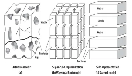
The DP formulation was first introduced by Barenblatt et al. (1960) who postulated that if a network of effectively connected “fissures” is present in a rock, mass transport from matrix to the fissures can be described by pseudo-steady state interporosity flow, which is also known as pseudo-steady dual porosity model. The authors assumed two overlapping continua and defined two average fluid pressures for every point in the domain, one for the matrix and one for the fissure/fracture (Figure 2.1). Warren and Root (1963) extended the solution to petroleum engineering applications. They represented the rock matrix as isotropic blocks enveloped by uniform and equally spaced fractures. Further, they introduced a shape factor to consider different matrix block shapes that controls the transmissivity between matrix and fractures. An example of a transfer (or interporosity flow) function that governs the flow from matrix to fractures is
, (2.1)
where σ is a shape factor that depends on the geometry of the matrix blocks, km is matrix
13
Kazemi (1969) presented a DP model with alternating layers of matrix and fractures, which is referred to as the slab model or transient fluid transfer model (Figure 2.1). The major difference of his model from the previous models was the consideration of transient flow in the matrix layers. de Swaan O. (1976) provided an analytical formulation of the transient flow model. In general, a storativity ratio ω, which is a measure of the contrast between the storativities of the matrix and fractures, and a transmissivity coefficient , which represents the contrast between the matrix and fracture conductivities, and an interporosity transfer function defines these models.
Figure 2.1: Dual-Porosity Idealization (Kuchuk and Biryukov 2013).
2.2 Dual-porosity/Dual-permeability Models
DPDK models are similar to the DP models with the exception that there is flow within the matrix blocks; i.e. matrix is not isolated and can directly communicate with the wellbore. The formulation includes matrix-fracture and matrix-matrix flow. Two separate continua are defined, one for matrix and one for fractures, and the flow is coupled between the two media. Such models can be constructed as an extension of the DP idealization of Barenblatt et al. (1960) or Kazemi (1969). Bourdet (1985) derived an analytical solution to compute the well response in a layered reservoir. The main objective of Bourdet’s solution was to identify cross-flow between the layers and the author showed that the DPDK approach is more suitable than the DP approaches when the reservoir includes thin layers with high contrast in permeability.
14
2.3 Discrete Fracture Network Models
In DFN models, each fracture is defined separately and fluid flow in and out of each fracture is formulated individually. Thus, this approach requires precise description of every fracture in the system (geometrical characterization, petrophysical and mechanical properties, and geological environment). Models can be constructed using deterministic or stochastic methods. With the emergence of aggregate characterization in later models, hierarchical patterns and chronological dependence were also incorporated into DFN models (Dershowitz and Einstein 1988).
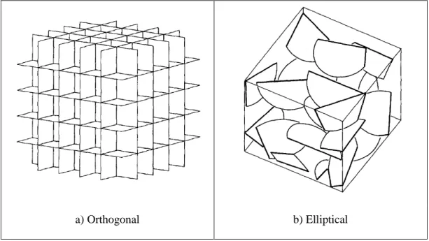
The orthogonal model shown in Figure 2.2a has been recognized and used in hydrology problems since the 1970s. Snow (1969) introduced the model using uniform spacing between orthogonal fractures. Conrad and Jacquin (1975) presented a DFN model that correlated between different fractures. Baecher and Lanney (1978) developed the disc- or elliptical-model shown in Figure 2.2b. The fractures are represented as discs of different sizes using deterministic or stochastic distribution in this approach. These discs can be terminated or connected at the edges of each block.
a) Orthogonal b) Elliptical
Figure 2.2: Examples of Deterministic and Stochastic DFN Models (Dershowitz and Einstein 1988).
15
Juanes et al. (2002) developed a model for single-phase flow in fractured reservoirs using finite-element methods. Matthai et al. (2005) presented a model for two-phase flow in fractured reservoirs using unconstructed 3D hybrid meshing and control-volume finite-element methods. DFN models require some techniques, such as control-volume finite-element and unconstructed gridding, and therefore are computationally expensive. In addition, an accurate DFN model is cumbersome since it demands precise 3D description of the fractures.
2.4 Fractals
O’Shaugnessy and Procaccia (1985) used fractals approach and presented a modified diffusion equation employing electric conductivity and current concepts. Their diffusion equation is given by
.
(2.2)In their formulation, the conductivity, k(r), is defined as the total conductivity of a spherical shell of radius r and it involves a product of spherically averaged value. The diffusion coefficient, K, is assumed to be constant and k(r) is defined as
, (2.3)
with Θ = D + α + 2 as the anomalous diffusion coefficient, D is the fractal dimension and α is the scaling power. The conductivity k(r) scales with the radial distance r based on a power-law and the Laplacian operator is modified by including the power index D. Thus, Eq. (2.2) is isotropic in D dimension(s) and the solution assumes a steady-state conductivity that is assigned spatially. The asymptotic solution curve for anomalous diffusion probability-density function displays a stretched shape. This formulation, however, neither provides the proper exponential function scaling nor meets the desired asymptotic behavior of the non-Gaussian probability function (Metzler et al. 1994).
Hewett (1986) provided a correlation to distribute reservoir properties using geostatistical parameters that correspond to a fractal system. The aim was to account for dispersion due to reservoir inhomogeneity and different scales of flow paths, which affect injected and recovered fluids. In modeling the reservoir, a Euclidean medium with statistical coefficients of fractional
16
Brownian motion (Brown 1827) were assumed. In addition, well log data were incorporated to distribute the properties.
Chang and Yortsos (1990) presented a solution for NFRs based on Eq. (2.2) with an objective to model natural fractures of different densities, conductivities and sizes. Also, they considered the natural fractures as a multi-fractal network (defined by certain fractal parameters) that is embedded in a Euclidean matrix. The equation governing fluid flow was given as
, (2.4)
where the superscripts d and D are the Euclidean and mass fractal dimension, respectively. With being the spectral or conductivity exponent in their derivation, was introduced as = D – – 1. In addition, the model accounted for pressure responses in two scenarios based on choosing the matrix to be interconnected or isolated from the well.
Beier (1994) also followed O’Shaugnessy and Procaccia (1985) and provided a solution for heterogeneous reservoirs. He utilized two domains to represent permeable and impermeable rocks with the permeable rock being a fractal network. Radial symmetry was assumed in obtaining the solution for a vertically fractured well with uniform flux and infinite-conductivity fracture as
, (2.5)
where ds is the spectral coefficient and df is the mass fractal coefficient. Also, = 2 + dw and df =
ds(2 + )/2. Using uniform flux and infinite conductivity, Beier (1994) was able to apply the
solution to field data. Also, he concluded that pressure expresses a power-law behavior during linear and radial flows.
Acuna and Yortsos (1995) used the solution by Chang and Yortsos (1990) and provided a numerical model for a synthetic fractal network combining the methods of fragmentation and iterated function system. They simulated the pressure transient response and concluded that well pressure is correlated with time by a power-law function. In addition, they were able to determine the spatial coefficient from the data.
17
Flamenco-Lopez and Camacho-Velázquez (2003) used the derivation from Chang and Yortsos (1990) and provided two solutions employing transient and pseudo-steady state matrix-to-fracture transfer function; one with matrix contribution to the flow and one without the contribution. Incorporating the pressure transient response from transient and pseudo-steady state flow periods, they were able to determine the parameters describing the fractal geometry.
Fuentes-Cruz et al. (2010) proposed a composite radial model with a fractal transitional zone to analyze build-up and fall-off tests. Their goal was to represent the viscous fingering developed during fluid injection as an intermediate fractal region between the invaded and non-invaded reservoir regions. In their formulation, the permeability and porosity of the fractal region change with distance by
(2.6)
and
(2.7)
The terms ϕ1 and k1 are porosity and permeability of the invaded region and r is the radius of the
fractal region bounded by the invaded and non-invaded areas (r1 < r < r2).
Cossio et al. (2012) derived a semi-analytical solution for an infinite single-porosity reservoir fully penetrated by a vertical fracture. Their solution was simplified to a form where porosity and permeability are spatially distributed with dimensionless distance raised to the exponents (df ‒ ‒ 2) for permeability and (df ‒ 2) for porosity, similar to Fuentes-Cruz et al
(2010). Their derivation for the Cartesian system can be transformed into radial flow by selecting proper scaling exponents. The authors stated that “a radial flow with constant hydraulic properties is equivalent to a linear flow with linearly increasing hydraulic properties” and the solution can be used to link linear and radial flows.
18
2.5 Anomalous Diffusion
Several attempts have been made to derive a proper AD equation as well as applying some of these solutions to reservoir engineering problems. Schneider and Wyss (1989) provided a solution in the form of fractional integral equation as
,
(2.8)where is the probability density, is the initial distribution, α = dw/2 and dw is the
anomalous diffusion exponent. However, this solution fails to provide the asymptotic shape of the distribution function since only one free parameter, α, is provided (Metzler et al. 1994).
Giona and Roman (1992) used spatial and temporal derivatives and obtained the following anomalous diffusion formulation
, (2.9)
where and ' ≥ 0. They utilized an explicit reference to account for diffusion temporally and applied a linear relationship between the radial current and the average probability density function. Their solution meets the asymptotic behavior of the non-Gaussian probability density function. Yet, the derived expression has some limitations and it does not reduce to the isotropic Gaussian (normal) diffusion when the parameters are set for such diffusion.
Metzler et al. (1994) provided a fractional diffusion equation in the form
. (2.10)
The parameters dw and ds In Eq. (2.10) are the diffusion exponent and spectral dimension,
respectively. This anomalous diffusion formulation is based on the relation that
(2.11)
and satisfies the asymptotic behavior of the non-Gaussian probability function. The temporal derivative carries the fraction (2/dw) and the spatial derivative carries (ds – 1). This solution
19
Camacho-Velázquez et al. (2008) provided a fractal fluid flow equation for NFRs using the diffusion equation derived by Metzler et al. (1994). The solution was derived for a fractal reservoir including and excluding the matrix contribution. With data from transient and boundary-dominated flow tests, pressure responses were used to estimate fractal parameters, characterize the NFR and compare results with O’Shaugnessy and Procaccia (1985) model ( = 0).
Raghavan (2011) used a Continuous-Time-Random-Walk model to derive a fractional equation for anomalous diffusion by including a fractional temporal derivative. Two models were provided; a radial flow model with symmetrical radial distribution of properties and a Cartesian model. Both solutions are applicable for production under constant rate or constant pressure. The equation for radial flow is given as
, (2.12)
where n is the dimension and would be replaced by the fractal coefficient df.
Fomin et al. (2011) showed that an anomalous diffusion equation can be derived by either relating a variable mass flux to spatial coordinates or assuming a scaled diffusion coefficient. They provide the following diffusion equation and mass flux law, respectively:
(2.13)
and
, (2.14)
where > 0 and < 1, which establishes fractional temporal and spatial derivatives, respectively. Chen and Raghavan (2013) revisited the expression in Raghavan (2011) and included the pseudo-skin function in the structure of the solution. They emphasized that the pseudo-skin function in their solution is time dependent and it would be independent of time if it were included in Chang and Yortsos (1990) or Beier (1994) formulations. Later, Chen and Raghavan (2015) published a 1D analytical solution following Metzler et al. (1994) diffusion equation. The
20
authors utilized temporal and spatial fractional derivatives and the solution was constructed assuming an infinite acting reservoir (open at one end). The solution provides options to set a constant production rate or constant production pressure condition.
2.6 Notable Models
In addition to the previous solutions, engineers and researchers have applied some techniques in effort to improve characterizing the porous structure and modeling fluid flow. One attempt is the triple-porosity models. Triple-porosity models are extensions of the DP approach in which a third system is introduced. Two main types can be found in the literature, I) two matrix systems and one fractures system and II) one matrix system and two fractures systems. The goal of these models is to account for changing properties in either matrix or fractures.
Abdassah and Ershaghi (1986) introduced a Type-I radial model applying unsteady-state matrix-to-fractures mass transfer. They utilized two idealizations; uniformly distributed blocks and strata as shown in Figure 2.3. Al-Ghamdi and Ershaghi (1996) developed a Type-II model to represent macro- and micro-fractures as more permeable and less permeable fractures, respectively, providing two derivations. First, the matrix feeds into micro-fractures, which feed into macro-fractures, all under pseudo-steady state flow. Second derivation is similar to the layered system with the micro-fractures replacing one matrix layer.
a) Strata b) Uniformly Distributed Blocks
21
Jalali and Ershaghi (1987) applied the strata idealization with Type-I model to study varying matrix properties. In addition, they looked into three combinations for the fluid transfer where 1) both matrix media under pseudo-steady flow, 2) both matrix media under unsteady flow and 3) one matrix medium under pseudo-steady flow and the other under unsteady flow.
Guo et al. (2012) presented a solution for a horizontal well in a vuggy fractured carbonate reservoir. Interporosity flow from vugs to matrix, vugs to fractures, and matrix to fractures were considered in their model.
Another method is the triple-continuum approach that was introduced by Liu et al. (2003). The reservoir rock is represented by fractures, matrix, and cavities, with pseudo-steady state flow between matrix and cavities. Only fractures are connected to the wellbore. Wu et al. (2004) utilized the triple-continuum approach by introducing small fractures, large fractures and rock matrix to model tracers and nuclear waste transport for water contamination studies.
Javadpour et al. (2007) proposed that gas flow in unconventional shale gas rocks should be modeled using Darcy flow in fractures and micro-pores, diffusive flow including viscous effects in the nano-pores, desorption from the kerogen surface to the nano-pores and diffusion within the kerogen.
Ozkan et al. (2009) developed a tri-linear model in which they included three contiguous regions: a hydraulic fracture, naturally-fractured inner reservoir and an outer reservoir. The model was used to conduct well test analysis for gas wells and the authors concluded that the outer reservoir contribution to fluid flow is negligible at extremely low matrix permeability.
Ozkan et al. (2010) introduced a dual-mechanism dual-porosity model by including advective and diffusive mechanisms to account for the details of flow between matrix and fractures. In addition, they considered stress-dependent fracture permeability and introduced a new matrix-fracture transfer function for unconventional NFRs.
Wu and Fakcharoenphol (2011) used multi-continuum approach to develop a numerical model that includes advective and diffusive flow and dispersion. The conservation equating included terms that accounted for mass accumulation via different fluid flow mechanisms. In their model they accounted for Darcy flow, Forchheimer effects, non-linear flow (Bingham
22
plastic), Klinkenberg effects, diffusive flow, sorption and geomechanical effects (stress-dependent porosity and permeability).
Ozcan et al. (2014) developed a tri-linear anomalous diffusion model by incorporating anomalous diffusion into the tri-linear model. Time-fractional flux governed diffusion in the inner reservoir region. They showed that anomalous diffusion is an effective tool that can be used to model fluid flow in heterogeneous porous media and it is a possible alternative to conventional models. In addition, it was highlighted that this approach does not require intrinsic properties for matrix and fracture, like DP models.
Holy and Ozkan (2016) presented an anomalous diffusion numerical solution to analyze production data from unconventional gas wells. The model includes spatial and temporal diffusion coefficients; flow is time and location dependent. For the analysis, super- or sub-diffusive flow signature is identified then the flow parameters are determined; namely the phenomenological permeability coefficient and the diffusion exponent. The analysis is rigorous and very convenient in providing the properties of the flow suggesting that AD is a promising modeling approach for unconventional reservoirs.
23
CHAPTER 3
ANALYTICAL MODEL
This chapter introduces the analytical model developed in this study. The details of the mathematical derivation are presented in Appendix A. Here, the general structure of the model is explained and the analytical solution is presented.
There are several key elements of the analytical model. It is built upon the tri-linear flow model, which was introduced as an approximation for flow toward fractured horizontal wells surrounded by a stimulated (naturally fractured) reservoir volume by Ozkan et al. (2009). As in the original TLM, the naturally fractured region between hydraulic fractures (SRV) is modeled by dual-porosity idealization. Because of the extremely tight matrix of unconventional reservoirs, transient fluid transfer from matrix to the fractures medium is assumed in the DP formulation (Kazemi 1969 and de Swaan O. 1976).
In the new model, a fractional flux law is used to account for anomalous diffusion in the fracture and matrix media instead of Darcy’s law used in the original TLM. Different anomalous diffusion exponents are allowed in the matrix and fractures. The fractional flux law defaults back to Darcy’s law for normal diffusion. This enables us to switch between normal and anomalous diffusion options in the matrix and fractures independently.
3.1 The Flux Law
Fluid flow in porous media is commonly modeled by Darcy’s law, which is given, in 1D, by
. (3.1)
Darcy’s law resulted from a series of macroscopic observations of flow through sand columns (Darcy 1856). Eq. (3.1) implies that the velocity of a moving fluid is directly proportional to the permeability k and the hydraulic head
. The permeability represents an average over length l and does not refer to a property at an exact point. Specifically, the velocity defined by Darcy’s
24
law is superficial velocity; that is, it defines bulk fluid movement between two points and the permeability is a bulk property (an average over space). Additional assumptions of Darcy’s law include continuum condition, viscous flow, and no-slip boundary (Hubbert 1963).
In statistical physics, the flux law given in Eq. (3.1) can be obtained by considering the random Brownian motion (Brown 1827) where displacement of the particles is represented by a Gaussian distribution; that is, the particles execute random and equally sized steps at discrete and equal time intervals. This diffusion process is referred to as normal diffusion. In normal diffusion, the probability of each particle moving to the next location is independent of the previous steps taken, both temporally and spatially. All probabilities to be in one of the next possible locations are equal and sum to unity. This suggests that the mean square displacement (MSD) is linearly scaled with time; that is,
. (3.2)
A more general approach can be taken by considering an uneven or anomalous displacement. This yields a power-law relationship between MSD and time, given by
, (3.3)
which results in a fractional or anomalous diffusion equation. Different processes, such as the Continuous-Time-Random-Walk or Levy Flights (LF), may be considered to arrive at this type of scaling of MSD with time. For example, a CTRW process is described by two functions, jumps and waiting times, with distinct probability functions as introduced by Montroll and Weiss (1965). For anomalous diffusion, a CTRW process leads to the following constitutive (flux) relation (Fomin et al., 2011, Raghavan 2011, Chen and Raghavan, 2015):
. (3.4)
The flux relation given in Eq. (3.4) for anomalous diffusion is the counterpart of Darcy’s law for normal diffusion. In this formulation 0 < α ≤ 1 and setting α = 1 defaults Eq. (3.4) to Eq. (3.1) and describes normal diffusion. This setup also dictates that a sub-diffusive process is expected as α deviates from unity; in other words, flow slows down as α decreases. The phenomenological constant, , does not carry the common units of permeability as in Darcy’s law. In field units,
25
has the units of (md∙Time1-α) instead of md, which signifies the memory-dependency of transport.
It must be noted that the use of the constitutive relation given by Eq. (3.4) in continuity equation leads to a time-fractional anomalous diffusion (sub-diffusion) equation. By also including a fractional space derivative in Eq. (3.4), a space- and time-fractional anomalous diffusion equation is obtained (Holy and Ozkan 2016). Turning off the time-fractional derivative (α = 1) but keeping space-fractional derivative yields a super-diffusion (space-fractional) anomalous diffusion formulation. Physically, sub-diffusion corresponds to an interpretation that the flow domain mainly consists of the more conductive medium and flow is interrupted or slowed down by randomly distributed, less conductive media or obstacles. Conversely, a super-diffusive process results from the acceleration of flow due to high-conductivity pathways or jumps in a less conductive main flow domain. In this work, only time-fractional anomalous diffusion (sub-diffusion) is considered.
3.2 General Approach, Assumptions, and Definitions
In this work, an analytical solution is derived for the bottomhole pressure of a multi-fractured horizontal well surrounded by an SRV in a tight unconventional reservoir. Flow of a single-phase, isothermal and slightly compressible fluid is considered. A fractional flux law that accounts for anomalous diffusion process is incorporated into the TLM idealization of flow toward a fractured horizontal well with an SRV. The naturally fractured SRV is modeled by the DP idealization and anomalous diffusion is considered independently in matrix and natural fractures with separate diffusion exponents. This approach allows for adapting different arrangements to consider various matrix and fracture properties. For instance, normal diffusion can be selected for well-connected natural fractures and sub-diffusion for heterogeneous or low-permeability matrix. Or else, sub-diffusion can be chosen for sparse or discontinuous natural fractures and normal diffusion for high-permeability matrix.
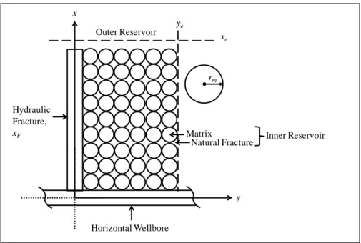
The TLM by Ozkan et al. (2009) is adopted for its applicability and utility in modeling unconventional NFRs. Figure 3.1 illustrates the employed DP idealization where the inner reservoir encloses uniform spherical matrix elements surrounded by a network of natural fractures. The dashed lines represent the flow boundaries parallel and perpendicular to the
26
wellbore, denoted by xe and ye, respectively. Three pressure solutions are derived for the outer
reservoir, inner reservoir and hydraulic fracture regions and coupled at their mutual boundaries. Pressure at the wellbore is computed by evaluating the hydraulic fracture pressure solution at the interface of the hydraulic fracture and the wellbore.
Figure 3.1: Illustration of the Symmetry Element and DP Idealization used in the Model.
The solution is derived in terms of scaled variables and in the Laplace transform domain. The results are inverted back to the real-time domain via Stehfest (1970) algorithm. In the presentation of the model, the subscript O is used for the outer reservoir region, subscripts f and m indicate natural fractures and matrix elements in the inner reservoir, respectively, and the properties of the hydraulic fracture are indicated by the subscript F. Scaled variables are denoted by the subscript D.
For normal diffusion, the scaled variables default back to the conventional dimensionless variables. For anomalous diffusion, however, scaled variables are not dimensionless. Although, it is possible to define a set of dimensionless variables for anomalous diffusion, for the comparison of the results with normal diffusion, the conventional definition of dimensionless variables are employed in this study. The following scaled variables are used in the derivations:
Outer Reservoir Hydraulic Fracture, xF Horizontal Wellbore x y Matrix
Natural Fracture Inner Reservoir rm
xe
27 , (3.5) , (3.6) , (3.7) , (3.8) , (3.9) , (3.10) , (3.11) and (3.12)
In addition, we define the bulk permeability of natural fractures by
. (3.13)
3.3 Overview of the Tri-Linear Flow Model
The TLM was developed for multiply fractured horizontal wells in low permeability shale reservoirs. As the name indicates, flow is assumed to be linear and coupled across the boundaries of three neighboring regions; outer reservoir, inner reservoir and the hydraulic fracture.
Flow equations for each region are constructed independently and solved by considering the continuity of pressure and flux at the interface of contiguous regions. The outer region is the reservoir beyond the hydraulic fracture tips and consists of the same matrix as the inner region (except, there are no natural fractures). The inner region is the reservoir bounded between the
28
hydraulic fractures and contains both the matrix and natural fractures. The model comprises several important assumptions including:
Linear flow is the dominant regime over the lifespan of fractured horizontal wells in shale reservoirs and in low permeability environments in general.
The wellbore is perforated at the location of the hydraulic fractures only.
Hydraulic fractures are equally spaced and have the same average properties ( , and ) and, therefore, the bisector of the distance between two consecutive hydraulic fractures is a no flow boundary.
Multiple stages of hydraulic fracturing can create and rejuvenate smaller fractures that act as a network for flow. Thus, vicinities of the hydraulic fractures (inner regions) can be considered as DP zones.
Hydraulic fractures are essential for production and flow in the inner reservoir region is normal to the hydraulic fractures.
At late times, after the inner reservoir is considerably depleted, the fractured horizontal well acts as a single hydraulic fracture and, therefore, flow from the outer reservoir is in the perpendicular direction of the wellbore.