Journal of Instrumentation
OPEN ACCESS
Fast simulation of muons produced at the SHiP experiment using
Generative Adversarial Networks
To cite this article: C. Ahdida et al 2019 JINST 14 P11028
View the article online for updates and enhancements.
2019 JINST 14 P11028
Published by IOP Publishing for Sissa Medialab
Received: September 13, 2019 Accepted: November 4, 2019 Published: November 27, 2019
Fast simulation of muons produced at the SHiP
experiment using Generative Adversarial Networks
The SHiP collaboration
C. Ahdida,44R. Albanese,14,d,hA. Alexandrov,14A. Anokhina,39S. Aoki,18G. Arduini,44 E. Atkin,38N. Azorskiy,29J.J. Back,54A. Bagulya,32F. Baaltasar Dos Santos,44A. Baranov,40 F. Bardou,44G.J. Barker,54M. Battistin,44J. Bauche,44A. Bay,46V. Bayliss,51
G. Bencivenni,15A.Y. Berdnikov,37Y.A. Berdnikov,37I. Berezkina,32M. Bertani,15 C. Betancourt,47I. Bezshyiko,47O. Bezshyyko,55D. Bick,8S. Bieschke,8A. Blanco,28 J. Boehm,51M. Bogomilov,1K. Bondarenko,27,55W.M. Bonivento,13J. Borburgh,44 A. Boyarsky,27,55R. Brenner,43D. Breton,4R. Brundler,47M. Bruschi,12V. Büscher,10 A. Buonaura,47S. Buontempo,14S. Cadeddu,13A. Calcaterra,15M. Calviani,44
M. Campanelli,53M. Casolino,44N. Charitonidis,44P. Chau,10J. Chauveau,5A. Chepurnov,39 M. Chernyavskiy,32K.-Y. Choi,26A. Chumakov,2P. Ciambrone,15L. Congedo,11, a
K. Cornelis,44M. Cristinziani,7A. Crupano,14,d G.M. Dallavalle,12A. Datwyler,47 N. D’Ambrosio,16G. D’Appollonio,13,cJ. De Carvalho Saraiva,28G. De Lellis,14,34,44,d M. de Magistris,14,d A. De Roeck,44M. De Serio,11, aD. De Simone,14,d L. Dedenko,39 P. Dergachev,34A. Di Crescenzo,14,d N. Di Marco,16C. Dib,2H. Dijkstra,44P. Dipinto,11, a V. Dmitrenko,38S. Dmitrievskiy,29L.A. Dougherty,44A. Dolmatov,30D. Domenici,15 S. Donskov,35V. Drohan,55A. Dubreuil,45M. Ehlert,6T. Enik,29A. Etenko,33,38F. Fabbri,12 L. Fabbri,12,b A. Fabich,44O. Fedin,36F. Fedotovs,52G. Felici,15M. Ferro-Luzzi,44
K. Filippov,38R.A. Fini,11P. Fonte,28C. Franco,28M. Fraser,44R. Fresa,14,iR. Froeschl,44 T. Fukuda,19G. Galati,14,dJ. Gall,44L. Gatignon,44G. Gavrilov,38V. Gentile,14,d S. Gerlach,6 B. Goddard,44L. Golinka-Bezshyyko,55A. Golovatiuk,14,d D. Golubkov,30A. Golutvin,52 P. Gorbounov,44D. Gorbunov,31S. Gorbunov,32V. Gorkavenko,55Y. Gornushkin,29 M. Gorshenkov,34V. Grachev,38A.L. Grandchamp,46G. Granich,32E. Graverini,46 J.-L. Grenard,44D. Grenier,44V. Grichine,32N. Gruzinskii,36A. M. Guler,48Yu. Guz,35 G.J. Haefeli,46C. Hagner,8H. Hakobyan,2I.W. Harris,46E. van Herwijnen,44C. Hessler,44 A. Hollnagel,10B. Hosseini,52M. Hushchyn,40G. Iaselli,11, a A. Iuliano,14,dV. Ivantchenko,32
2019 JINST 14 P11028
R. Jacobsson,44D. Joković,41M. Jonker,44I. Kadenko,55V. Kain,44B. Kaiser,8 C. Kamiscioglu,49K. Kershaw,44M. Khabibullin,31E. Khalikov,39G. Khaustov,35 G. Khoriauli,10A. Khotyantsev,31S.H. Kim,22Y.G. Kim,23V. Kim,36,37N. Kitagawa,19 J.-W. Ko,22K. Kodama,17A. Kolesnikov,29D.I. Kolev,1V. Kolosov,35M. Komatsu,19
N. Kondrateva,32A. Kono,21N. Konovalova,32,34S. Kormannshaus,10I. Korol,6I. Korol’ko,30 A. Korzenev,45V. Kostyukhin,7E. Koukovini Platia,44S. Kovalenko,2I. Krasilnikova,34 Y. Kudenko,31,38,g E. Kurbatov,40P. Kurbatov,34V. Kurochka,31E. Kuznetsova,36 H.M. Lacker,6M. Lamont,44G. Lanfranchi,15O. Lantwin,52A. Lauria,14,dK.S. Lee,25 K.Y. Lee,22J.-M. Lévy,5V.P. Loschiavo,14,hL. Lopes,28E. Lopez Sola,44V. Lyubovitskij,2 J. Maalmi,4A. Magnan,52V. Maleev,36A. Malinin,33Y. Manabe,19A.K. Managadze,39 M. Manfredi,44S. Marsh,44A.M. Marshall,50A. Mefodev,31P. Mermod,45A. Miano,14,d
S. Mikado,20Yu. Mikhaylov,35D.A. Milstead,42O. Mineev,31A. Montanari,12M.C. Montesi,14,d K. Morishima,19S. Movchan,29Y. Muttoni,44N. Naganawa,19M. Nakamura,19T. Nakano,19 S. Nasybulin,36P. Ninin,44A. Nishio,19A. Novikov,38B. Obinyakov,33S. Ogawa,21
N. Okateva,32,34B. Opitz,8J. Osborne,44M. Ovchynnikov,27,55N. Owtscharenko,7
P.H. Owen,47P. Pacholek,44A. Paoloni,15B.D. Park,22S.K. Park,25A. Pastore,11M. Patel,52 D. Pereyma,30A. Perillo-Marcone,44G.L. Petkov,1K. Petridis,50A. Petrov,33D. Podgrudkov,39 V. Poliakov,35N. Polukhina,32,34,38J. Prieto Prieto,44M. Prokudin,30A. Prota,14,d
A. Quercia,14,d A. Rademakers,44A. Rakai,44F. Ratnikov,40T. Rawlings,51F. Redi,46 S. Ricciardi,51M. Rinaldesi,44Volodymyr Rodin,55Viktor Rodin,55P. Robbe,4
A.B. Rodrigues Cavalcante,46T. Roganova,39H. Rokujo,19G. Rosa,14,dT. Rovelli,12,b O. Ruchayskiy,3T. Ruf,44V. Samoylenko,35V. Samsonov,38F. Sanchez Galan,44
P. Santos Diaz,44A. Sanz Ull,44A. Saputi,15O. Sato,19E.S. Savchenko,34J.S. Schliwinski,6 W. Schmidt-Parzefall,8N. Serra,47S. Sgobba,44O. Shadura,55A. Shakin,34
M. Shaposhnikov,46P. Shatalov,30T. Shchedrina,32,34L. Shchutska,46V. Shevchenko,33 H. Shibuya,21L. Shihora,6S. Shirobokov,52A. Shustov,38S.B. Silverstein,42S. Simone,11, a R. Simoniello,10M. Skorokhvatov,38,33S. Smirnov,38J.Y. Sohn,22A. Sokolenko,55
E. Solodko,44N. Starkov,32,33L. Stoel,44B. Storaci,47M.E. Stramaglia,46D. Sukhonos,44 Y. Suzuki,19S. Takahashi,18J.L. Tastet,3P. Teterin,38S. Than Naing,32I. Timiryasov,46 V. Tioukov,14D. Tommasini,44M. Torii,19N. Tosi,12D. Treille,44R. Tsenov,1,29S. Ulin,38 A. Ustyuzhanin,40Z. Uteshev,38G. Vankova-Kirilova,1F. Vannucci,5P. Venkova,6V. Venturi,44 S. Vilchinski,55M. Villa,12,bHeinz Vincke,44Helmut Vincke,44C. Visone,14,d K. Vlasik,38 A. Volkov,32,33R. Voronkov,32S. van Waasen,9R. Wanke,10P. Wertelaers,44J.-K. Woo,24 M. Wurm,10S. Xella,3D. Yilmaz,49A.U. Yilmazer,49C.S. Yoon,22P. Zarubin,29I. Zarubina29 and Yu. Zaytsev30
1Faculty of Physics, Sofia University, Sofia, Bulgaria
2Universidad Técnica Federico Santa María and Centro Científico Tecnológico de Valparaíso, Valparaíso, Chile
3Niels Bohr Institute, University of Copenhagen, Copenhagen, Denmark 4LAL, Univ. Paris-Sud, CNRS/IN2P3, Université Paris-Saclay, Orsay, France
5LPNHE, IN2P3/CNRS, Sorbonne Université, Université Paris Diderot,F-75252 Paris, France 6Humboldt-Universität zu Berlin, Berlin, Germany
2019 JINST 14 P11028
8Universität Hamburg, Hamburg, Germany
9Forschungszentrum Jülich GmbH (KFA), Jülich, Germany
10Institut für Physik and PRISMA Cluster of Excellence, Johannes Gutenberg Universität Mainz, Mainz, Germany
11Sezione INFN di Bari, Bari, Italy 12Sezione INFN di Bologna, Bologna, Italy 13Sezione INFN di Cagliari, Cagliari, Italy 14Sezione INFN di Napoli, Napoli, Italy
15Laboratori Nazionali dell’INFN di Frascati, Frascati, Italy 16Laboratori Nazionali dell’INFN di Gran Sasso, L’Aquila, Italy 17Aichi University of Education, Kariya, Japan
18Kobe University, Kobe, Japan 19Nagoya University, Nagoya, Japan
20College of Industrial Technology, Nihon University, Narashino, Japan 21Toho University, Funabashi, Chiba, Japan
22Physics Education Department & RINS, Gyeongsang National University, Jinju, Korea 23Gwangju National University of Education,eGwangju, Korea
24Jeju National University,eJeju, Korea 25Korea University, Seoul, Korea
26Sungkyunkwan University,eSuwon-si, Gyeong Gi-do, Korea 27University of Leiden, Leiden, The Netherlands
28LIP, Laboratory of Instrumentation and Experimental Particle Physics, Portugal 29Joint Institute for Nuclear Research (JINR), Dubna, Russia
30Institute of Theoretical and Experimental Physics (ITEP) NRC ’Kurchatov Institute’, Moscow, Russia 31Institute for Nuclear Research of the Russian Academy of Sciences (INR RAS), Moscow, Russia 32P.N. Lebedev Physical Institute (LPI), Moscow, Russia
33National Research Centre ’Kurchatov Institute’, Moscow, Russia
34National University of Science and Technology "MISiS", Moscow, Russia
35Institute for High Energy Physics (IHEP) NRC ’Kurchatov Institute’, Protvino, Russia 36Petersburg Nuclear Physics Institute (PNPI) NRC ’Kurchatov Institute’, Gatchina, Russia 37St. Petersburg Polytechnic University (SPbPU),f St. Petersburg, Russia
38National Research Nuclear University (MEPhI), Moscow, Russia
39Skobeltsyn Institute of Nuclear Physics of Moscow State University (SINP MSU), Moscow, Russia 40Yandex School of Data Analysis, Moscow, Russia
41Institute of Physics, University of Belgrade, Serbia 42Stockholm University, Stockholm, Sweden
43Uppsala University, Uppsala, Sweden
44European Organization for Nuclear Research (CERN), Geneva, Switzerland 45University of Geneva, Geneva, Switzerland
46École Polytechnique Fédérale de Lausanne (EPFL), Lausanne, Switzerland 47Physik-Institut, Universität Zürich, Zürich, Switzerland
48Middle East Technical University (METU), Ankara, Turkey 49Ankara University, Ankara, Turkey
2019 JINST 14 P11028
51STFC Rutherford Appleton Laboratory, Didcot, U.K. 52Imperial College London, London, U.K.
53University College London, London, U.K. 54University of Warwick, Warwick, U.K.
55Taras Shevchenko National University of Kyiv, Kyiv, Ukraine aUniversità di Bari, Bari, Italy
bUniversità di Bologna, Bologna, Italy cUniversità di Cagliari, Cagliari, Italy
dUniversità di Napoli “Federico II”, Napoli, Italy
eAssociated to Gyeongsang National University, Jinju, Korea
fAssociated to Petersburg Nuclear Physics Institute (PNPI), Gatchina, Russia
gAlso at Moscow Institute of Physics and Technology (MIPT), Moscow Region, Russia hConsorzio CREATE, Napoli, Italy
iUniversità della Basilicata, Potenza, Italy
E-mail: alex.marshall@cern.ch
Abstract: This paper presents a fast approach to simulating muons produced in interactions of the SPS proton beams with the target of the SHiP experiment. The SHiP experiment will be able to search for new long-lived particles produced in a 400 GeV/c SPS proton beam dump and which travel distances between fifty metres and tens of kilometers. The SHiP detector needs to operate under ultra-low background conditions and requires large simulated samples of muon induced background processes. Through the use of Generative Adversarial Networks it is possible to emulate the simulation of the interaction of 400 GeV/c proton beams with the SHiP target, an otherwise computationally intensive process. For the simulation requirements of the SHiP experiment, generative networks are capable of approximating the full simulation of the dense fixed
target, offering a speed increase by a factor of O(106). To evaluate the performance of such an
approach, comparisons of the distributions of reconstructed muon momenta in SHiP’s spectrometer between samples using the full simulation and samples produced through generative models are presented. The methods discussed in this paper can be generalised and applied to modelling any non-discrete multi-dimensional distribution.
Keywords: Detector modelling and simulations I (interaction of radiation with matter, interaction of photons with matter, interaction of hadrons with matter, etc); Simulation methods and programs
2019 JINST 14 P11028
Contents1 Introduction 1
2 The SHiP experiment 2
3 The SHiP simulation 3
4 Generative adversarial networks 4
5 GANs for the SHiP experiment 6
5.1 Pre-processing 6
5.2 Figure of merit 6
5.3 Network optimisation and GAN architecture 7
6 GAN performance 8
7 Reconstructing GAN generated muons 10
8 Benchmarking 12
9 Conclusion 13
1 Introduction
Generative networks are a class of machine learning algorithms designed to generate samples according to a multidimensional function, given a randomly distributed input sample. Generative networks have been studied in the machine learning community primarily for the purpose of image generation. Each image in a training set is made up of a multitude of pixels, corresponding to a data point in a high dimensional space. Within this space, underlying features of the set of images are encoded through dependencies between pixels. Generative networks attempt to model the characteristics that define a specific set of training images. These models can then be used to generate images that are faithful emulations of the original training set. Generative networks have been successfully employed for a variety of applications such as: generating high quality images that obey fundamental features of training set images; the generation of images from descriptive
text [1]; modelling image captions [2]; producing photo realistic super resolution images [3]; and
generating high resolution images from semantic mapping [4,5].
Searches for physics beyond the Standard Model often involve looking for rare signatures and must therefore be able to suppress background processes which can be many orders of magni-tude more abundant than the signal. In order to optimise the design of the detectors, develop reconstruction algorithms and understand the efficiency of the selection criteria, large samples of
2019 JINST 14 P11028
simulated background events are required. Dedicated software packages such as GEANT4 [6] model
the transport of particles through the material and the detector response. In many cases, the CPU requirements to simulate these interactions with matter prohibit the production of large numbers of background events due to the computationally expensive procedure. Therefore, the computing
demands of the simulation of high energy physics experiments are increasing exponentially [7].
Recent algorithmic improvements that take advantage of high performance computing resources
aim at reducing simulation time, resulting in an order of magnitude increase in speed [8]. This
im-provement is not sufficient to meet the demands of future particle physics experiments, such as those
at the High Luminosity LHC, for large simulation samples [7]. Generative neural networks offer
an alternative approach to simulation by modelling non-analytical functions in a computationally
efficient way [9].
The use of generative networks for particle physics originally focused on image based gen-eration. Examples of their application include: the development of Location Aware Generative
Adversarial Networks for the production of images of jets [10]; the simulation of reconstructed
cosmic ray induced air showers [11], and of showers in electromagnetic calorimeters [12]; the
fast simulation of Cherenkov detectors [13]. More recently, generative approaches have also been
adopted to simulate the kinematics of final state particles emerging from physical exclusive
two-to-two processes, such as Z or top-quark production at the LHC [14,15]. In ref. [16], generative
networks were used to simulate the detector reconstruction of the Z → µ+µ−process at the LHC.
This paper describes the use of generative networks to emulate the kinematics of muons produced through the interactions of high energy protons with the dense target designed for the
Search for Hidden Particles (SHiP) experiment [17]. This approach offers a gain of multiple orders
of magnitude in the computational efficiency of such processes. In contrast to the aforementioned use of generative networks to approximate a single exclusive process, this work employs four different generative networks to model the kinematics of muons originating from a multitude of processes, including muons from secondary interactions or particle showers in SHiP’s target. Large samples of generative based muons can then be passed through the GEANT4 based simulation of the rest of the SHiP experiment, offering a precise modelling of its detector response and reconstruction.
This paper is organised as follows: sections2and3describe the SHiP detector and its simulation
framework respectively; section 4 discusses the generative models used in this analysis, while
section5details how these networks are trained and optimised for the SHiP experiment. Section6
and7then present the performance of the generative models in simulating muons produced through
interactions of high energy protons with the SHiP target, compared to the Pythia8 [18] and GEANT4
frameworks. Finally, section8discusses the computational time required to produce muons through
generative networks.
2 The SHiP experiment
The Search for Hidden Particles experiment (SHiP) is a proposed experiment that will operate at the the prospective general purpose fixed target facility at the CERN Super Proton Synchrotron (SPS) accelerator. The SHiP experiment aims to search for long-lived exotic particles with masses between
a few hundred MeV/c2and a few GeV/c2. These particles are expected to be produced in the decays
of heavy hadrons. The facility is therefore designed to maximise the production rate and detection
2019 JINST 14 P11028
SHiP has received a large amount of attention from the particle physics community. The SHiPphysics paper [2] is a highly cited document (see Figure 1), and many groups continue to explore the sci-entific potential of the experiment, making detailed predictions for models of feebly interacting particles. In the wake of the SHiP experiment, several dedicated intensity frontier experiments have been pro-posed in the recent years: CODEX-b [46], MATHUSLA [47–49], FASER [50–52]. Recognising the importance of diversifying the search efforts, the CERN Management created in 2016 a dedicated study group “Physics Beyond Colliders” (PBC) [5]. Searches for heavy neutral leptons, dark photons, dark scalars, light dark matter, and other super-weakly interacting light particles has also been included in the scientific goals of many presently running experiments [39, 40, 42–44, 44, 53–67].
1.3 Overview of the SHiP developments and advances since the TP
Despite an active program of searches for HS particles in many experiments, SHiP remains a unique dedicated experiment capable of reconstructing the decay vertex of an HS particle, measuring its invariant mass and providing particle identification of the decay products in an environment of extremely low background. Moreover, SHiP is also optimised to search for LDM through scattering signatures and for tau neutrino physics.
Since the Technical Proposal the SHiP design went through a significant re-optimisation phase. Figure 2 shows the layout of the re-optimised SHiP detector. While the overall set-up of the detector remains unchanged, the geometry and the detector composition has been significantly modified, and technological studies and test beams have brought maturity to the design. SHiP consists of the proton
Figure 2: Overview of the SHiP experiment as implemented in FairShip.
target, followed by a hadron stopper and an active muon shield that sweeps muons produced in the beam dump out of acceptance. Since the TP, the target has been extended from ten to twelve interaction lengths in order to reduce the hadronic shower leakage. Studies were made to minimise the distance between the target and the SHiP spectrometers to improve the acceptance of the spectrometers, and to reduce the weight and cost of the muon shield. A significant improvement was achieved by starting the first section of the muon shield within the hadron stopper by integrating a coil which magnetises the iron shielding blocks.
The SHiP detector itself incorporates two complementary apparatuses, the Scattering and Neutrino Detector (SND), and the Hidden Sector (HS) spectrometer. The SND will search for LDM scattering and perform neutrino physics. It is made of an emulsion spectrometer located inside a single long magnet with a field above 1.2 T in the entire volume, and a muon identification system. The emulsion spectro-meter is a hybrid detector consisting of alternating layers of an absorber, nuclear emulsion films and fast electronic trackers. The absorber mass totals ⇠ 10 tonnes.
The HS decay spectrometer aims at measuring the visible decays of HS particles by reconstructing their decay vertices in a 50 m long decay volume. In order to eliminate the background from neutrinos
5
Figure 1. SHiP facility layout [19].
efficiency for charm and beauty mesons and their decay products, while maintaining the lowest possible background rate. The 400 GeV/c proton beam extracted from the SPS will be dumped on
a high density W/Mo target with the aim of accumulating 2 × 10²⁰protons on target during 5 years
of operation. The charm production at SHiP will exceed that of any existing or planned facility. The
SHiP detector, shown in figure1, incorporates two complementary apparatuses, the Scattering and
Neutrino Detector (SND), and the Decay Spectrometer (DS). The SND will be used to search light dark matter particles, and perform neutrino physics measurements. The DS aims at measuring the visible decays of hidden sector particles by reconstructing their decay vertices in a 50 m long decay volume, making use of a magnetic spectrometer, veto systems and particle identification detectors.
Further details of the design of the detector can be found in ref. [19]. Such a setup will allow the
SHiP experiment to probe a variety of models that predict light long-lived exotic particles.
Since particles originating in charm and beauty meson decays are produced with a significant
transverse momentum with respect to the beam axis,1the detector is placed as close as possible
to the target. The high flux of muons produced in the target represents a serious background in
searches for hidden particles. A critical component of the SHiP experiment is the muon shield [20],
which deflects muons produced in the target away from the detector placed downstream of the target. The SHiP detector is designed to reconstruct the exclusive decays of hidden particles and to reduce the background to less than 0.1 events in the full five year period of operation.
3 The SHiP simulation
The simulation of the various physics processes of the response of the SHiP detector are handled
by the FairShip software suite, which is based on the FairRoot software framework [21].
Within FairShip, primary collisions of protons are generated with Pythia8 and the subsequent propagation and interactions of particles are simulated with GEANT4. Neutrino interactions are
simulated with GENIE [22], while heavy flavour production and inelastic muon interactions with
Pythia6[23] and GEANT4. Secondary heavy flavour production in cascade interactions of hadrons
originating from the initial proton collision with the SHiP target is also taken into account [24].
The pattern recognition algorithms used to reconstruct tracks from the hits on the strawtubes of the
DS are described in [25], and the algorithms for particle identification are presented in [26].
2019 JINST 14 P11028
In order to optimise the design of the active muon shield, and develop the reconstructionand selection algorithms of the SHiP experiment, a large simulation campaign was undertaken. Muons produced in the SHiP target were simulated with momentum p > 10 GeV/c and a sample
corresponding to approximately 1011 protons on target was produced. In order to enhance this
sample with muons likely to enter the DS, the cross-section of muons produced from decays of
ρ0, ω, η and η0mesons was enhanced by a factor of 100. Similarly, the cross-section for photon
conversions into muon pairs was also enhanced by the same factor. The full simulation of this
sample, corresponding to a fraction of the 4 × 10¹³protons-on-target SPS spill, required months of
running on dedicated CPU farms. An order of magnitude increase of this sample could be achieved by exploiting symmetries of the system, such as that in the azimuthal plane of the collision. However,
generating even larger samples commensurate to the 2 × 10²⁰SPS protons on target expected during
the lifetime of the experiment is impossible using conventional particle simulation methods. The simulation of the initial proton interaction with the SHiP target, including the subsequent secondary interactions of particles with the target and the hadron absorber, requires significant computing
power. Methods such as SMOTE [27] and ADASYN [28] could be used to synthesise a sample of
muons that is larger than the original fully simulated sample. These methods rely on producing muons whose position and momentum vectors take values that lie in between those of existing muons in the fully simulated sample. Generative adversarial networks can offer an alternative way of producing orders of magnitude larger samples with minimal expense to the fidelity of the generated muons.
4 Generative adversarial networks
Neural networks model functions that map an n-dimensional input parameter space into an m-dimensional output, and are widely employed in the particle physics community. A traditional neural network is built up of multiple layers: an input layer, one or more intermediate hidden layers, and an output layer. Layers are built from many individual nodes, and a pattern of connections joins nodes in adjacent layers. Each node has an associated tunable bias term that acts as an activation threshold of the node, and each connection has an associated tunable weight representing the strength of the connection. The simplest pattern of connections between layers is one were the nodes in one layer are fully connected with nodes in the adjacent layer. In this configuration the output value of each node is calculated by firstly calculating the sum of the output values of each node from the previous layer, weighted by the strength of each connection. This weighted sum is then shifted by the bias term and passed through an activation function that modulates the output of a node. Depending on the layer that a particular node belongs to, different types of activation functions can be used. For instance, hidden layers often make use of the so called “leaky rectified
linear unit” function [29] and in the final layer a sigmoid function could be used to transform the
output into a value between 0 and 1. This choice would be appropriate in a binary classification network, whose output is an estimate of whether the input sample originated from one out of two classes of samples.
A neural network must be trained in order for it to successfully approximate a function. The training process involves tuning and updating the weight and bias parameters of the network, with “supervised learning” being the most traditional approach to training. In the first stage of a
2019 JINST 14 P11028
binary classification problem, labelled data are passed through the network. Output values are thenrecorded and compared to the true labels through the use of a loss function. The loss function provides a quantitative measure of the network’s performance on a set of input training samples. A large value of the loss function indicates that the network is unable to distinguish between the two classes of samples. The value of the loss function is used in a process called back-propagation to update the weight and bias parameters across the network in an effort to improve the network’s
performance [30]. Neural networks are trained in steps, where in each step a small batch of training
data is used, the loss function is then evaluated using this batch of data, and the weight and bias parameters of the network are updated for the next step.
Generative Adversarial Networks (GANs) employ two competing neural networks, one acting
as a generator and the other as a discriminator [31]. The generator ˆG is trained to map an input
vector of random noise z to an output generated vector G(z; θg), where θg are parameters of the
network and the dimensionality of z is typically larger than that of G(z; θg). The discriminator ˆD,
with trainable parameters θd, is trained to map an input vector x to an output prediction D(x; θd),
which is a value between 0 and 1. In the study presented in this paper G(z; θg) and x represent
the momentum and position vector of the muons. The value of D(x; θd) represents the probability
that x originated from the training sample. A value of D(x; θd) closer to 0 indicates that ˆDexpects
the sample to have been generated by ˆG, whereas if D(x; θd) is closer to 1 ˆDis predicting that the
sample originated from the training data.
The discriminator and generator networks are trained using an iterative approach. Firstly, the discriminator is trained to distinguish between generated and training samples via a binary
crossentropy loss function Ld. This is a common loss function for training classifier networks and
is defined as
Ld = −[ytruelog(ypred)+ (1 − ytrue) log(1 − ypred)], (4.1)
where ytruetakes the values of 1 or 0 for the training or generated label of the sample respectively,
and ypred is the predicted label by the discriminator given by ypred = D(x; θd). The value of this
loss function increases rapidly the further ypred is from the ytrue. Large values of the loss function
bring significant changes in the values of trainable parameters θdin the network.
The generator network is then trained in a stacked model which directly connects the output
xgenof ˆGto the discriminator prediction D(xgen; θd). This is the adversarial component of the GAN,
it is only the feedback of ˆDthat influences the training of ˆG. The xgen never directly affects the
training of ˆG. In this stacked model all training parameters of the discriminator, θd, are fixed to the
values obtained from the previous training step of ˆD. The trainable parameters, θg, of the generator
are updated based on the loss function, Lg, whose value depends on the output of the discriminator
and is defined as
Lg = − log(D(xgen; θd)). (4.2)
Low values of D(xgen; θd) indicate that the discriminator is confident that the sample xgenoriginated
from the generator, leading to a large value of Lg. Generated samples that closely resemble
training samples will return higher values of D(xgen; θd) and consequently lower values of Lgas the
discriminator is successfully tricked into guessing a sample originated from the training sample. The training of the discriminator and generator is repeated using the samples generated by
2019 JINST 14 P11028
indistinguishable from training samples. Different approaches are employed to determine the endof the training. In this paper the metric used to monitor the quality of the training is discussed in
section5.2. The overall accuracy of the generator depends on how well the discriminator is trained
to distinguish between generated and training samples.
5 GANs for the SHiP experiment
The GAN is trained on a sample of 3.4 × 10⁸muons passing through the target and hadron absorber
in the full simulation campaign discussed in section 3. As mentioned, this training sample is
artificially enriched with muons from rare processes. Therefore, in order to obtain a physical admixture of muons from various sources, batches of muons are extracted from the training sample according to a probability that corrects for this enhancement.
Training is performed on the position r and momentum p vectors of these muons at their point of production. Therefore, the GAN generates position and momentum vectors of muons at their production point within the target. Subsequently, they are propagated through the active muon shield and the Decay Spectrometer, relying on GEANT4 to simulate muon interactions with matter. This procedure allows for a fast production of large muon samples, while maintaining the flexibility to optimise the magnetic shield and downstream detector elements of SHiP, as well as the ability to correct for effects due to the spatial distribution of the proton beam impinging on the target.
Four separate GANs are trained, separated by muon charge and prompt or displaced origin.
The x- and y-coordinates of muons originating from prompt decays of mesons such as the ρ0, φ
and J/ψ are always the same. This is a consequence of the training sample that relies on Pythia with no smearing of the proton-beam distribution. As such, muons from prompt sources are treated separately from muons originating from other sources. Therefore, the GANs trained on prompt muons generate four features (z, p), and the GANs for non-prompt muons generate six (r, p). In this approach correlations between muons produced in pairs from, for example, vector-meson decays are ignored. Muons are generated individually and any correlation is assumed to be lost via the multiple scattering of the muons through the hadron absorber and muon shield.
5.1 Pre-processing
The distribution of the x- and y- coordinates of muons from non-prompt sources is extremely peaked
around the interaction point. Therefore, each value of the x (y) distribution xi(yi) is transformed as
xitrans= (
−p| xi− x| if xi < 0,
p
| xi− x| if xi > 0, (5.1)
before training the GANs. This transformation widens the distributions, which proves easier for the GANs to model. The distributions of all the input features are then normalised to values between -1 and 1. This transformation is reversed to obtain physical values of the generated output.
5.2 Figure of merit
An important requirement of the full simulation of the SHiP detector is to accurately model the flux of muons reaching the Decay Spectrometer. This flux crucially depends on the momentum
2019 JINST 14 P11028
distribution of the muons entering the muon shield of the SHiP experiment. Therefore, muonsgenerated through the GAN approach must closely match the kinematic distributions of the muons produced in the target using the full simulation.
In order to optimise the architecture of the networks and to quantify the quality of the training procedure a figure of merit, FoM, is developed with the following requirements. The FoM must account for how well the GAN is able to model individual features and the correlations between them. Furthermore, it is important that the FoM offers an independent metric of the quality of the training of the GAN since the discriminator and the generator of the GAN improve in tandem during the iterative training procedure. Finally, the calculation of the FoM must be fast so that it does not slow down the training process.
During the training process, small test samples are generated to test the progress of the procedure. As the number of muon features can span a six dimensional space, a small generated
sample of muons results in a sparsely populated feature space. Therefore, traditional binned
goodness of fit methods, such as χ2-tests, break down as almost all bins in this space have a low
occupancy. Boosted decision trees can overcome this issue [32] and satisfy the aforementioned
requirements on the FoM.
A gradient boosted decision tree, BDT, is trained periodically to distinguish between generated and fully simulated muon samples. The BDT uses 100,000 muons generated from the latest GAN configuration and 100,000 randomly selected, fully simulated muons. Half of the muons in each sample are used for training and the other half for testing. The resulting performance of the BDT is quantified through the area under the receiver operating characteristic curve (ROC AUC). A generated sample that is indistinguishable from a fully simulated sample would return an ROC AUC value of 0.5.
5.3 Network optimisation and GAN architecture
All networks are trained with a mini-batch gradient descent approach [33] and at each training step
the networks use a sub-sample of training data. The generators and discriminators of the GANs are built using only fully connected layers, resulting in a GAN performance that is independent of the ordering of the muon parameters in the vectors of features that make up the training sample. The number of nodes, the size of the batch sub-sample, the number of layers and the learning rate of the networks are coarsely optimised through a grid search over these parameters. The four GANs are
trained until the ROC AUC of the BDT based FoM described in section5.2flattens out, and the
selected architecture is that which minimises the ROC AUC of the FoM.
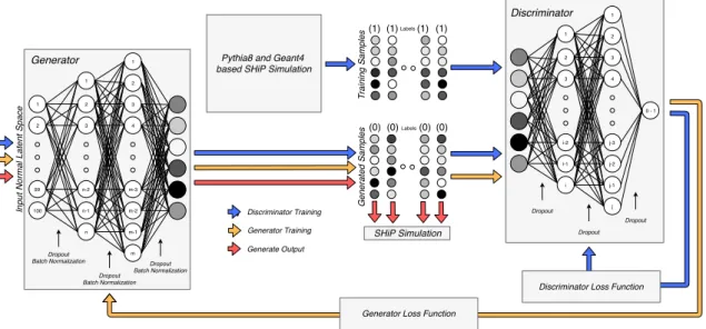
As a result of this optimisation procedure, the GANs for both prompt and non-prompt muons
follow the architecture shown in figure2. Leaky rectified linear unit activation functions are used
at every hidden layer. The generator and the discriminator have two hidden layers in an inverted pyramidal structure. For the prompt muon GANs, the number of nodes in each hidden layer of
ˆ
G are 1536 and 3072 and for ˆD are 768 and 1536. For the non-prompt GANs, the number of
corresponding nodes are 512 and 1024 for ˆGand 768 and 1536 for ˆD. The input to the generators
relies on sampling from a latent space given by a 100 dimensional unit Gaussian distribution. The
last layer of ˆGhas a tanh activation function in accordance to the transformed range of the input
features described in section5.1. The last layer of ˆDhas a sigmoid activation function providing an
2019 JINST 14 P11028
1 2 99 100 1 1 2 3 2 3 4 n n-1 n-2 m m-1 m-2 m-3Input Normal Latent Space
1 1 2 3 2 3 4 i i-1 i-2 j j-1 j-2 j-3 0 - 1 Generator Discriminator
Pythia8 and Geant4 based SHiP Simulation
T raining Samples (1)(1) (1) (1) (0) (0) (0) (0) Generated Samples Generator Training Discriminator Training Generate Output Labels Labels
Generator Loss Function
SHiP Simulation
Discriminator Loss Function Dropout Batch Normalization Dropout Batch Normalization Dropout Batch Normalization Dropout Dropout Dropout
Figure 2. Optimal GAN architecture obtained for the simulation of muon background in SHiP. The number
of nodes in each layer for prompt µ and non-prompt µ GANs are given in the text. Arrows indicate the flow of samples and loss information for each stage of training and generation. The features in the generated and training samples can take values between -1 and 1 as denoted by the varying shades of grey.
a dropout probability of 0.25 are added between each layer of ˆGand ˆDto prevent overfitting [34].
Batch normalisation layers are also added between layers of ˆG[35].
For this study the Adam optimisation algorithm [36] was used in training the networks.
Em-ploying the AMSgrad algorithm with the Adam optimiser increased the stability of our output loss
and FoM progress with training [37]. A momentum parameter of Adam, βl, is used with a value of
0.5 to control the progress of the gradient descent during the training of the network.
6 GAN performance
The progress of the FoM throughout the training of each GAN, as well as the BDT distributions
of the optimal GAN models are shown in figure3. The final FoM values for the prompt µ+and
µ−GAN models are 0.57 and 0.54 respectively. Whereas, the non-prompt µ+and µ−GAN models
return FoM values of 0.60 and 0.59 respectively. A more sophisticated optimisation procedure
of the network architecture, such as that suggested in [38], could result in an even better GAN
performance.
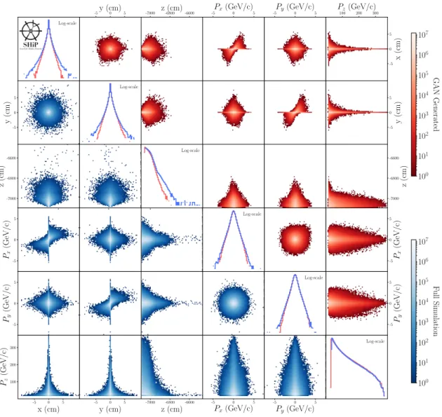
In order to further visualise the level of agreement between the generated and fully simulated samples, a physical sample of GAN based muons is produced by combining the output from each of the four generators according to the expected production fractions of prompt and non-prompt muons
in the simulation. Figure4 compares the one- and two-dimensional distributions of each unique
pair of features between fully simulated and generated muons. The GANs can overall reproduce the correct correlations between features, although the tails of the (x, y, z) position distributions are underestimated.
2019 JINST 14 P11028
Training Progress 0.5 0.6 0.7 0.8 0.9 1.0 F oM (R OC A UC) Prompt µ− Non-prompt µ− Prompt µ+ Non-prompt µ+ (a) 0 0.25 0.5 0.75 1 Non-prompt µ− BDT Response 0 1000 2000 3000 4000 0 0.25 0.5 0.75 Non-prompt µ+ BDT Response 0 1000 2000 3000 0 0.25 0.5 0.75 Prompt µ− BDT Response 0 2000 4000 6000 Generated Fully Simulated 0 0.25 0.5 0.75 Prompt µ+ BDT Response 0 2000 4000 6000 (b)Figure 3. (a) Progress of the FoM ROC AUC value throughout the training of all 4 GANs, raw and smoothed
data is displayed. Dashed lines indicate the FoM AUC ROC values of models chosen to generate muons in this paper. Although models were trained past this point this was the lowest FoM AUC ROC value obtained, (b) Distributions of the figure of merit BDT response for both fully simulated and GAN-based muon samples
for prompt and non-prompt µ−and µ+.
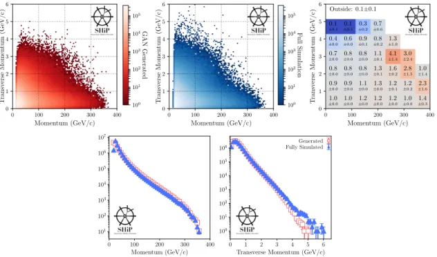
Modelling of the momentum (p) and transverse momentum (pT) plane accurately is crucial
in order to obtain the correct flux of muons reaching the SHiP Decay Spectrometer. Figure 5
compares the (p, pT) plane between the fully simulated and generated samples. The GANs can
largely reproduce the correlations between these features, however they particularly underestimate
the number of muons with pT > 3 GeV/c. The effect of this mismodelling on the rate and kinematics
of muons reaching the Decay Spectrometer is discussed in section7. To correct the momentum
distribution of the generated muons, the three-dimensional (px, py, pz) distributions of the fully
simulated and generated muons are each fit using a three-dimensional Kernel Density Estimator,
for example see ref. [39]. For each generated muon, an individual correction weight is derived
by taking the ratio between fully simulated over the fully generated KDEs at the corresponding
(px, py, pz) muon coordinate.
This generative approach accurately models the production of muons in the SHiP target, as long as the kinematic distributions of the muons lie within the phase space covered by the fully simulated training sample. Therefore, samples of muons produced through the GAN are designed to compliment, rather than replace, existing fully simulated samples. By generating vast samples of muons through this generative approach, a better understanding of the performance of the muon shield and the detector response for muons that lie within the kinematic region of the fully simulated sample can be obtained.
2019 JINST 14 P11028
-5y (cm)0 5 -7000 z (cm)-6800 -6600 -5Px(GeV/c)0 5 -5Py(GeV/c)0 5 P100z(GeV/c)200 300
-5 0 5 x (cm) -5 0 5 y (cm) -7000 -6800 -6600 z (cm) -5 0 5 Px (GeV/c) -5 0 5 Py (GeV/c) 100 101 102 103 104 105 106 107 GAN Generated -5 0 5 y (cm) -7000 -6800 -6600 z (cm) -5 0 5 Px (GeV/c) -5 0 5 Py (GeV/c) -5 0 5 x (cm) 100 200 300 Pz (GeV/c) -5 0 5 y (cm) -7000 -6800 -6600 z (cm) -5 0 5 Px(GeV/c) -5 0 5 Py(GeV/c) 100 101 102 103 104 105 106 107 F ull Sim ulation Log-scale Log-scale Log-scale Log-scale Log-scale Log-scale
Figure 4. Two-dimensional distributions of all unique combinations of muon features for GAN based
(upper-half) and fully simulated (lower-half) muons produced in the SHiP target. One-dimensional log scale comparisons of each feature are presented along the diagonal.
7 Reconstructing GAN generated muons
The generated muons are processed using FairShip to simulate their passage through the magnetic
shield and the response of the downstream SHiP detector. Figure6shows the p vs pTdistribution
of reconstructed muon tracks in the Decay Spectrometer of SHiP resulting from the GAN based muon sample. A comparison to the reconstructed muon tracks originating from the full simulation sample is also shown. The effect of the residual correction to the kinematics of the GAN based
muon sample discussed in section6is found to have a small effect.
Figure 7shows the momentum distributions at the production point of the muons, for muons
that are reconstructed in the DS. The GAN based and fully simulated muons display similar features
in the p vs pTplane. The fully simulated sample exhibits localised hot-spots. These are due to the
use of event weights that account for enhancement factors of particular processes that give rise to
muons likely to enter the Decay Spectrometer as discussed in section3.
2019 JINST 14 P11028
0 100 200 300 400 Momentum (GeV/c) 0 1 2 3 4 5 6 T ransv erse Momen tum (GeV/c) 100 101 102 103 104 105 GAN Generated 0 100 200 300 400 Momentum (GeV/c) 0 1 2 3 4 5 6 T ransv erse Momen tum (GeV/c) 100 101 102 103 104 105 F ull Sim ulation 0 100 200 300 400 Momentum (GeV/c) 0 1 2 3 4 5 6 T ransv erse Momen tum (GeV/c) Outside: 0.1±0.1 1.0 ±0.0 0.9 ±0.0 0.8 ±0.0 0.7 ±0.0 0.4 ±0.0 0.1 ±0.1 1.0 ±0.0 0.9 ±0.0 0.8 ±0.0 0.8 ±0.0 0.6 ±0.0 0.1 ±0.1 1.2 ±0.0 1.1 ±0.0 0.8 ±0.0 0.8 ±0.0 0.9 ±0.1 0.3 ±0.2 1.2 ±0.0 1.3 ±0.0 1.3 ±0.1 1.1 ±0.1 0.8 ±0.2 0.7 ±0.6 1.2 ±0.0 1.2 ±0.1 1.6 ±0.2 4.1 ±1.4 1.3 ±1.0 1.0 ±0.0 1.2 ±0.2 2.8 ±1.5 3.0 ±2.4 1.4 ±0.3 2.3 ±1.6 1.0 ±1.4 0 100 200 300 400 Momentum (GeV/c) 101 102 103 104 105 106 107 0 1 2 3 4 5 6Transverse Momentum (GeV/c)
100 101 102 103 104 105
106 Fully SimulatedGenerated
Figure 5. Two-dimensional p vs pTdistributions for GAN based (top-left), fully simulated (top-middle)
and the ratio (top-right) of muons produced in the SHiP target. The comparisons of the one dimensional
projections for p (bottom-left) and pT(bottom-right) are also shown.
0 100 200 300
Track Momentum (GeV/c) 0 200 400 600 800 1000 1200 1400 1600 10−1 100 101 102
Track Momentum (GeV/c) 0 200 400 600 800 Generated Generated (weighted) Fully Simulated
Figure 6. Distribution in linear (left) and log-scale (right) of the reconstructed track momentum of muons
in the Decay Spectrometer. The distributions of both GAN based and fully simulated muons are also shown together with the effect of the correction to the residual mismodelling of the muon kinematics from the GAN based sample. The distributions are normalised such that they correspond to the same number of protons on target.
The rate of muons that survive the magnetic shield and are reconstructed in the Decay
Spec-trometer is given in table 1. Both the full rate, and the rate of muons with an initial (p, pT)
2019 JINST 14 P11028
and fully simulated muon samples. The correction to the kinematic distributions of the GAN basedmuons discussed in section6, changes the rate of generated muons entering the Decay Spectrometer
by ∼ 4%.
Table 1. Rates of reconstructed muons in the Decay Spectrometer. The uncertainty on the GAN based muons
reflects the statistical uncertainty of the generated muon sample, given the model described in section6.
Approach Full Rate (kHz) Upper Region Rate (kHz)
Full simulation 13.9 ± 3.4 4.7 ± 2.2 GAN 15.8 ± 0.3 5.5 ± 0.2 GAN (weighted) 15.2 ± 0.5 4.7 ± 0.4
Momentum (GeV/c)
0 100 200 300 0 1 2 3 4 5 6T
ransv
erse
Momen
tum
(GeV/c)
Fully Simulated 0 100 200 300 400 GAN Generated 10−5 10−4 10−3 10−2 10−1 100 101 102Figure 7. Initial momentum of muons passing through the SHiP active muon shield with well reconstructed
tracks in the Decay Spectrometer. Full simulation data is presented on the left and generated data on the
right. The dashed line indicates the upper region analysed in table1.
8 Benchmarking
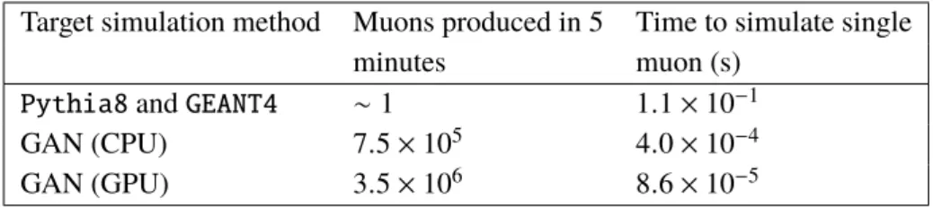
With a small expense in the fidelity between the generated and fully simulated sample, the generative approach can produce samples of muons at greater speed. Generating samples of muons from GANs
on a GPU provides a speed-up of O(106) relative to the full Pythia8 and GEANT4 proton-on-target
simulation. This test was performed using Keras(v2.1.5) on a TensorFlow backend (v1.8.0) on a single Nvidia Pascal P100 GPU card. This speed-up factor includes all the computations required to transform the output features of the generator into physical values. Generating muons using the GAN approach on a CPU is an order of magnitude slower than on a GPU.
Table2summarises the results of this performance test. The gain in speed using the generative
approach is partly due to the small production cross-section of muons with p > 10 GeV/c, requiring
O(103) proton-on-target interactions to be simulated through Pythia8 in order to generate a
single muon.
2019 JINST 14 P11028
Table 2. Summary of benchmarking results.
Target simulation method Muons produced in 5 Time to simulate single
minutes muon (s)
Pythia8and GEANT4 ∼ 1 1.1 × 10⁻¹
GAN (CPU) 7.5 × 10⁵ 4.0 × 10⁻⁴
GAN (GPU) 3.5 × 10⁶ 8.6 × 10⁻⁵
9 Conclusion
This paper demonstrates the success of using a modern machine learning method to approximate the output of a complex and computationally intensive simulation of muons originating from SPS protons impinging on the target of the SHiP experiment. The GAN models presented in this paper produce samples that emulate the characteristics of the fully simulated sample and can approximate the kinematic correlations of the muons produced in the SHiP target. Furthermore, muons generated by these GANs correctly describe the expected flux and kinematic distributions of muons that survive the magnetic shield and are reconstructed in the Decay Spectrometer of the SHiP detector.
The generative models developed in this paper can produce muons O(106) times faster than
the current Pythia8 and GEANT4 simulation of the SHiP target. However, the muons produced by the generative model are only representative of regions of phase space populated by the full simulation of the target. These generative models are not capable of accurately extending the tails of their training distributions, and are not intended to replace the fully simulated background sample. Generated muons can be used in parallel to complement ongoing background and detector optimisation studies, where this approach can offer a vast increase in the sample size of statistically limited muon background studies at SHiP. Finally, the generative approach presented in this paper can be used to produce muons according to a model trained directly on real data, such as that
from the recent muon-flux beam-test campaign of the SHiP collaboration [40]. Such an approach
circumvents the challenge of tuning the multitude of parameters that control the simulation in order to match the data.
Acknowledgments
This work was carried out using the computational facilities of the Advanced Computing Research
Centre, University of Bristol —http://www.bristol.ac.uk/acrc/. We would like to thank the NVIDIA
corporation for the donation of a Titan Xp which was used for this research.
The SHiP Collaboration wishes to thank the Castaldo company (Naples, Italy) for their con-tribution to the development studies of the decay vessel. The support from the National Re-search Foundation of Korea with grant numbers of 2018R1A2B2007757, 2018R1D1A3B07050649, 2018R1D1A1B07050701, 2017R1D1A1B03036042, 2017R1A6A3A01075752,
2016R1A2B4012302, and 2016R1A6A3A11930680 is acknowledged.
The support from the FCT — Fundação para a Ciência e a Tecnologia of Portugal with grant number CERN/FIS-PAR/0030/2017 is acknowledged. The support from the Russian Foundation for Basic Research (RFBR), grant 17-02-00607, the support from the TAEK of Turkey, and the
2019 JINST 14 P11028
support from the U.K. Science and Technology Facilities Council (STFC), grant ST/P006779/1 areacknowledged.
We thank M. Al-Turany, F. Uhlig. S. Neubert and A. Gheata their assistance with FairRoot. We acknowledge G. Eulisse and P.A. Munkes for help with Alibuild.
We thank M. Daniels for his contributions to the construction of the liquid-scintillator testbeam detectors.
The muon flux and charm cross section measurements this summer would not have been possible without a significant financial contribution from CERN. In addition, several member institutes made large financial and in-kind contributions to the construction of the target and the spectrometer sub detectors, as well as providing expert manpower for commissioning, data taking and analysis. This help is gratefully acknowledged.
References
[1] H. Zhang et al., Stackgan: Text to Photo-realistic Image Synthesis with Stacked Generative
Adversarial Networks,arXiv:1612.03242.
[2] Y. Pu et al., Variational Autoencoder for Deep Learning of Images, Labels and Captions, in Advances
in neural information processing systems. Proceedings of Neural Information Processing Systems
2016, Barcellona Spagna (2016) [arXiv:1609.08976].
[3] C. Ledig et al., Photo-Realistic Single Image Super-Resolution Using a Generative Adversarial
Network,IEEE Conf. Comput. Vis. Pattern Recognit. 2017(2017) 1[arXiv:1609.04802].
[4] T. Wang et al., High-Resolution Image Synthesis and Semantic Manipulation with Conditional GANs,
IEEE Conf. Comput. Vis. Pattern Recognit. 2018(2018) 1[arXiv:1711.11585].
[5] P. Isola, J. Zhu, T. Zhou and A.A. Efros, Image-to-Image Translation with Conditional Adversarial
Networks,arXiv:1611.07004.
[6] GEANT4 collaboration, GEANT4: A Simulation toolkit,Nucl. Instrum. Meth. A 506(2003) 250.
[7] HEP Software Foundation collaboration, A Roadmap for HEP Software and Computing R&D
for the 2020s,Comput. Softw. Big Sci. 3(2019) 7[arXiv:1712.06982].
[8] P. Canal et al., GeantV: from CPU to accelerators,PoS(ICHEP2016)177.
[9] M. Mirza and S. Osindero, Conditional Generative Adversarial Nets,arXiv:1411.1784.
[10] L. de Oliveira, M. Paganini and B. Nachman, Learning Particle Physics by Example: Location-Aware
Generative Adversarial Networks for Physics Synthesis,Comput. Softw. Big Sci. 1(2017) 4
[arXiv:1701.05927].
[11] M. Erdmann, J. Glombitza and D. Walz, A Deep Learning-based Reconstruction of Cosmic
Ray-induced Air Showers,Astropart. Phys. 97(2018) 46[arXiv:1708.00647].
[12] M. Paganini, L. de Oliveira and B. Nachman, CaloGAN: Simulating 3D high energy particle showers
in multilayer electromagnetic calorimeters with generative adversarial networks,Phys. Rev. D 97
(2018) 014021[arXiv:1712.10321].
[13] D. Derkach, N. Kazeev, F. Ratnikov, A. Ustyuzhanin and A. Volokhova, Cherenkov Detectors Fast
Simulation Using Neural Networks, in 10th International Workshop on Ring Imaging Cherenkov
Detectors (RICH 2018), Moscow Russia (2018) [arXiv:1903.11788].
[14] A. Butter, T. Plehn and R. Winterhalder, How to GAN LHC Events,arXiv:1907.03764.
[15] S. Otten et al., Event Generation and Statistical Sampling for Physics with Deep Generative Models
and a Density Information Buffer,arXiv:1901.00875.
2019 JINST 14 P11028
[16] B. Hashemi, N. Amin, K. Datta, D. Olivito and M. Pierini, LHC analysis-specific datasets with
Generative Adversarial Networks,arXiv:1901.05282.
[17] SHiP collaboration, A facility to Search for Hidden Particles (SHiP) at the CERN SPS,
arXiv:1504.04956.
[18] T. Sjöstrand, S. Mrenna and P.Z. Skands, A Brief Introduction to PYTHIA 8.1,Comput. Phys.
Commun. 178(2008) 852[arXiv:0710.3820].
[19] SHiP collaboration, SHiP Experiment — Progress Report,CERN-SPSC-2019-010(2019).
[20] SHiP collaboration, The active muon shield in the SHiP experiment,2017 JINST 12 P05011
[arXiv:1703.03612].
[21] M. Al-Turany et al., The FairRoot framework,J. Phys. Conf. Ser. 396(2012) 022001.
[22] C. Andreopoulos et al., The GENIE Neutrino Monte Carlo Generator,Nucl. Instrum. Meth. A 614
(2010) 87[arXiv:0905.2517].
[23] T. Sjöstrand, S. Mrenna and P.Z. Skands, PYTHIA 6.4 Physics and Manual,JHEP 05(2006) 026
[hep-ph/0603175].
[24] H. Dijkstra and T. Ruf, Heavy Flavour Cascade Production in a Beam Dump,
CERN-SHiP-NOTE-2015-009(2015).
[25] E. Van Herwijnen, T. Ruf, M. Ferro-Luzzi and H. Dijkstra, Simulation and pattern recognition for the
SHiP Spectrometer Tracker,CERN-SHiP-NOTE-2015-002(2015).
[26] B. Hosseini and W.M. Bonivento, Particle Identification tools and performance in the SHiP
Experiment,CERN-SHiP-NOTE-2017-002(2017).
[27] N.V. Chawla, K.W. Bowyer, L.O. Hall and W.P. Kegelmeyer, SMOTE: synthetic minority
over-sampling technique,J. Artif. Intell. Res. 16(2002) 321[arXiv:1106.1813].
[28] H. He, Y. Bai, E.A. Garcia and S. Li, ADASYN: Adaptive synthetic sampling approach for imbalanced
learning,IEEE Int. Joint Conf. Neural Netw. 2008(2008) 1
[29] A.L. Maas, A.Y. Hannun and A.Y. Ng, Rectifier Nonlinearities Improve Neural Network Acoustic
Models, Proc. ICML 30 (2013) 3.
[30] D.E. Rumelhart, G.E. Hinton and R.J. Williams, Learning representations by back-propagating
errors, Cognitive Modeling 5 (1988) 1 [Nature 323(1988) 533].
[31] I.J. Goodfellow et al., Generative Adversarial Networks,arXiv:1406.2661.
[32] C. Weisser and M. Williams, Machine learning and multivariate goodness of fit,arXiv:1612.07186.
[33] S. Ruder, An overview of gradient descent optimization algorithms,arXiv:1609.04747.
[34] N. Srivastava et al., Dropout: A Simple Way to Prevent Neural Networks from Overfitting, J. Mach.
Learn. Res. 15(2014) 1929.
[35] S. Ioffe and C. Szegedy, Batch Normalization: Accelerating Deep Network Training by Reducing
Internal Covariate Shift,arXiv:1502.03167.
[36] D.P. Kingma and J. Ba, Adam: A Method for Stochastic Optimization,arXiv:1412.6980.
[37] S.J. Reddi, S. Kale and S. Kumar, On the Convergence of Adam and Beyond,arXiv:1904.09237.
[38] M. Jaderberg et al., Population Based Training of Neural Networks,arXiv:1711.09846.
[39] D.W. Scott, Multivariate density estimation: theory, practice, and visualization, John Wiley & Sons, New York U.S.A. (2015).
[40] SHiP collaboration, Alignment of the muon-flux spectrometer in FairShip using the survey