2015:53 Ductile tearing – Micromechanical analyses and experimental study

Research

Report number: 2015:53 ISSN: 2000-0456 Available at www.stralsakerhetsmyndigheten.se

Ductile tearing – Micromechanical

analyses and experimental study

2015:53

SSM 2015:53

SSM perspective Background

In a previous published research work (SSM 2014:28) it was studied how the Gurson model will be used to predict ductile crack growth at the presence of secondary stresses, e.g. weld residual stresses. Accord-ing to this study, the experimental load-deformation correlation could be predicted by using FEM-analyses for the initiation of crack growth in specimens containing residual stresses. Since the initiation of crack growth is rarely critical for ductile materials, it was of interest to predict the correlation of load-deformation for a more general geometry con-taining a crack growing in a ductile way. Additional experiments were also performed to investigate the effect of load history on the fracture toughness of a ductile material as well as the ability of the Gurson model to deal with these effects.

The study showed that there is a need for further experimental work and analysis to better understand the material behaviour at different levels of pre-loading.

Objective

The aim of the project is to further develop the previous work in order to achieve the goal to simulate ductile crack growth in experiments or other situations where the influence of the secondary stresses is domi-nating.

Results

Some of the conclusions are as follows:

• For specimens pre-loaded to 8% of total strain at room temperature in both tension and compression, large effects are seen on both the tearing resistance and crack initiation.

• An effect from the pre-load is also seen for the specimens pre-loaded to 4.5% total strain. This applies for pre-loading in both tension and compression. However, the effect on the fracture toughness is greater in the specimens pre-loaded in tension.

• The shear modified Gurson model does not overestimate the fracture resistance, as was seen for the standard Gurson model.

Need for further research

Currently there is no need for further research. Project information

Contact person SSM: Kostas Xanthopoulos Reference: SSM2013-4357

2015:53

Author:

Date: December 2015

Report number: 2015:53 ISSN: 2000-0456 Available at www.stralsakerhetsmyndigheten.se

Tobias Bolinder

Inspecta Technology AB , Stockholm, Sweden

Ductile tearing – Micromechanical

analyses and experimental study

This report concerns a study which has been conducted for the Swedish Radiation Safety Authority, SSM. The conclusions and view-points presented in the report are those of the author/authors and do not necessarily coincide with those of the SSM.

Summary

In this report, the project “Ductile Tearing-Micromechanical analyses and experimental study” is presented. In the project, numerical cell modeling has been conducted using the shear modified Gurson model proposed by Nahshon and Hutchinson [1] to evaluate its capability in predicting the effect of residual stresses. Experimental work has also been conducted for material characterization. The material used in the experiments was A533B-1.

The computational work done shows that the cell model does capture the effects attributable to residual stresses, as seen in the experimental work by Bolinder et al. [2]. From the predicted results presented in Chapter 5.3 the same conclusions that were made from the experimental results in [2] can be drawn with regard to fracture toughness and the decreasing influence on the J-integral for increasing primary load. The predictions made here also show an improvement when using the shear modified Gurson model compared with earlier predictions in [3], where the standard Gurson model was used.

The results presented in this report lead to the conclusion that using the cell modeling technique is a sound approach in studying the effects from residual stresses on ductile fracture at low primary loads.

Sammanfattning

Denna rapport syftar till att presentera projektet “Ductile tearing - Micromechanical analyses and experimental study”. Projektet omfattar numerisk mikromekanisk modellering med hjälp av en materialmodell som har utvecklats av Nahshon och Hutchinson [1] samt ett experimentellt arbete för att bestämma materialegenskaper. Materialmodellen är en Gurson modell som har modifierats för att kunna hantera skjuvdominerade spänningsfällt. I det utförda arbetet undersöktes materialmodellens förmåga att prediktera duktil spricktillväxt i situationer med höga restspänningar. I det experimentella arbetet användes materialet A533B-1. Det genomförda numeriska arbetet visar att den skjuvmodifierade Gurson modellen [1] klarar att prediktera effekterna av ett restspänningsfällt, som kunde observeras i tidigare experiment utförda av Bolinder et al. [2]. De slutsatser som kunde tas utifrån det experimentella arbetet i [2] kunde även tas utifrån de numeriska resultaten med avseende på restspänningsfältets effekt på last-CMOD kurvor, brottsegheten, och även återge det minskande inflytandet på J-integralen från restspänningarna för ökande primär last. Resultaten i denna rapport visade även på en förbättring vid användandet av den skjuvmodofierade Gurson modellen i jämförelse med tidigare utfört arbete av Bolinder [3] där standard Gurson modellen använts.

De redovisade resultaten i denna rapport leder till slutsatsen att användandet av cellmodellering för att undersöka effekten från restspänningsfällt på duktilt brott är ett bra och tillförlitligt tillvägagångssätt.

Contents

ACKNOWLEDGEMENT ... 4

1 INTRODUCTION ... 5

2 THEORETICAL BACKGROUND ... 6

FRACTURE MECHANICS OF DUCTILE TEARING ... 6

2.1 MICROMECHANICAL MODELING OF DUCTILE TEARING ... 6

2.2 2.2.1 Gurson model ... 7

2.2.2 Shear modified Gurson model ... 8

DETERMINE CELL MODEL PARAMETERS ... 9

2.3 3 EXPERIMENTAL PROGRAM ... 12 SHEAR TEST... 14 3.1 PRE-LOADING ... 14 3.2 FRACTURE TESTING ... 15 3.3 4 EXPERIMENTAL RESULTS AND DISCUSSION ... 16

SHEAR TESTS ... 16

4.1 FRACTURE TESTS ... 16

4.2 5 PREDICTIONS USING CELL MODELLING ... 22

FE-MODELS ... 23

5.1 5.1.1 Shear specimen ... 23

5.1.2 Fracture specimen ... 24

DETERMINING THE CELL MODEL PARAMETERS ... 26

5.2 EVALUATION OF THE CAPABILITY OF THE CELL MODELING TECHNIQUE IN CAPTURING THE EFFECTS OF 5.3 RESIDUAL STRESSES ... 30 6 DISCUSSION ... 34 7 CONCLUSIONS ... 35 8 FUTURE WORK ... 35 REFERENCES ... 36

Acknowledgement

The author is grateful for the financial support of the Swedish Radiation Safety Authority, Forsmark, Ringhals, OKG and TVO. This project was conducted in close collaboration with the department of Solid Mechanics at KTH, where the theoretical expertise received from Jonas Faleskog during the project and the experimental expertise from Martin Öberg are very much appreciated. The author would also like to thank AMEC UK for assisting in supplying the material used in the experiments.

1 Introduction

Cracked components are usually subjected to loads causing both primary and secondary stresses. In welds the main contribution to secondary stresses is usually weld residual stresses. Engineering assessment methods, such as the ASME section XI code and the R6 procedure, are commonly used to conduct assessments of such components. How these codes treat secondary stresses differ. ASME section XI code does not consider secondary stresses in some materials while the R6 method on the other hand sometimes tends to give overly conservative assessments. In Sweden the contribution from the secondary stresses and the primary stresses to KI or J is treated as equally important for components subjected to low primary loads, i.e low Lr (Lr=load/limit-load) values (Lr <0.8). But for high primary loads (Lr >0.8) the contribution from the secondary stresses is weighted down according to the procedure developed by Dillström et al. in [4]. This treatment of secondary stresses has been verified experimentally by Bolinder et al. [2]. To experimentally examine the contribution of secondary stresses, in particular weld residual stresses, to KI or J at low primary loads (low Lr values) is more complicated and practically difficult. Hence, to be able to numerically simulate these kinds of experiments would be very beneficial. This is possible with a model describing the micromechanical process of ductile tearing, such as the Gurson model.

Earlier studies have already shown good predictions of JR-curves using micromechanical modeling with the Gurson model, studies have also determined the ability to account for constraint and size effects with the Gurson model, see the work done by Gao et al. [5] [6]. The ability for the Gurson model to handle residual stresses was shown earlier by Bolinder [3]. In [3] it was however suggested that better predictions could be made with a Gurson model incorporating damage buildup due to shear. One such model has been developed by Nahshon and Hutchinson [1].

The goal of the work described in this report is to evaluate the ability of the shear modified Gurson model by Nahshon Hutchinson [1] in predicting the effect from residual stresses. This is a necessary step towards the future and final goal, which would be to simulate ductile initiation and tearing in conditions with high residual stresses. This could possibly give a basis to lower the contribution from the residual stresses to KI or J at low primary loads (low Lr values) in engineering assessments, provided that the material behavior is ductile.

In this report, the project “Ductile tearing – Micromechanical analyses and experimental study” is described. The report contains the theoretical background to ductile fracture and micromechanical modeling, the experimental program with a discussion of the results, the micromechanical modeling and resulting numerical predictions and a discussion of the numerical and experimental results and finally conclusions drawn from the work.

2 Theoretical background

Fracture mechanics of ductile tearing

2.1

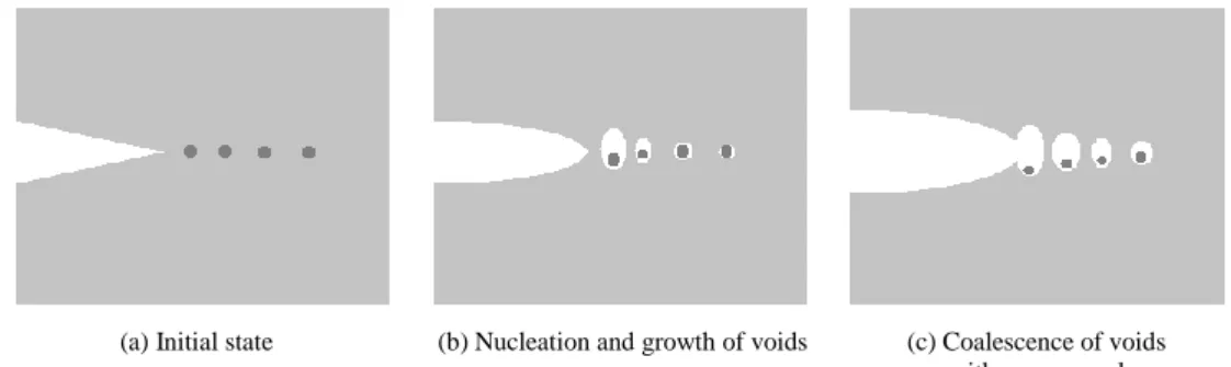
Ductile fracture in common structural and pressure vessel steels is characterized by the forming and coalescence of microvoids from impurities such as inclusions and second phase particles. As large plastic deformations on the microscopic level develop in front of the macroscopic crack, voids nucleate from inclusions, as the load is increased the formed microvoids grow. Finally microvoids from second phase particles such as carbide inclusions coalescence and assist the tearing of the ligaments between the enlarged voids. This process creates a weakened band in front of the macroscopic crack, allowing an extension of the macroscopic crack. These mechanisms are driven by the combination of high triaxial stresses and high plastic strains ahead of the macroscopic crack. Nucleation of voids typically occurs for particles at a distance of ~2δ (CTOD) from the crack tip, while the void growth occurs much closer to the crack tip relative to CTOD (crack tip opening displacement). The process of ductile crack growth is illustrated in Figure 0.1 below.

(a) Initial state (b) Nucleation and growth of voids (c) Coalescence of voids with macro crack

Figure 0.1. Mechanics of ductile crack growth.

Micromechanical modeling of ductile tearing

2.2

With a cell model the growth and coalescence of voids and the interaction between the fracture process zone and the background material is modeled. By describing the ductile tearing with a cell model there is a possibility to study the influence of different parameters on ductile fracture.

With a cell model the material in the fracture process zone is modeled by an aggregate of similarly sized cells which form a material layer with the height D, as illustrated in Figure 0.2.

Figure 0.2. Illustration of cell modeling of ductile tearing.

The cell model approach was originally proposed by Xia and Shih [7] [8]. Each cell is a three dimensional element with dimension D comparable to the spacing between large inclusions. Each cell contains a spherical void of initial volume fraction f0. The material outside the cell layer is modeled as standard elasto-plastic continuum. The damage mechanism in the cell layer, void growth and coalescence is commonly modeled using Gurson’s constitutive relation [9] with modification introduced by Tvergaard [10]. In this work the shear modified Gurson model is used which was introduced by and Nahshon, Hutchinson [1].

2.2.1 Gurson model

The Gurson model is a homogenized material model where spherical voids are treated in a smeared out fashion. The form of the yield condition Φ(σe,σh,σf,f)=0 used in this report, which is incorporated in the finite element code ABAQUS [11], applies to strain hardening materials with isotropic hardening as follows

0

1

2

3

cosh

2





























q

f

q

q

f









where f is the current void volume fraction, σe the macroscopic effective Mises stress, σh the macroscopic hydrostatic stress and σf the current matrix flow strength. The parameters q1 and q2 were introduced by Tvergaard [10] to improve model predictions.

Ductile crack growth occurs when a cell loses its stress carrying capacity by strain softening due to void growth that cannot be compensated for by material strain hardening. This process is not accurately captured by the Gurson model. Tvergaard and Needleman [12] therefore proposed to model this process as follows: When the void volume fraction f reaches a critical value of fc, the void growth is increased

rapidly to the point when the void volume fraction reaches fE, at which point total failure at the material point occurs and once all the elements material points fail the element is rendered extinct. The parameters fc and fE are user specified. In ABAQUS this is modeled by the following function,

























f

f

f

f

f

f

f

f

f

f

f

f

f

f

if

)

(

if

1

q

f



In this report the form of the Gurson model described above will henceforth be referred to as the standard Gurson model. This model is incorporated in the commercial ABAQUS software.

2.2.2 Shear modified Gurson model

In the standard Gurson model damage growth or material softening in pure shear cannot be predicted. This is since no void growth is predicted at zero triaxiality under pure shear using the standard Gurson model. Therefore Nashson and Hutchinson in [1] proposed a modification to the Gurson model. The proposed model was introduced to take into account the damage growth and material softening due to void deformation and reorientation experienced in materials subjected to shear loads.

The only modification to the standard Gurson model done by Nahshon and Hutchinson is the change of the equation governing the increment of void growth 𝑓̇. The modification adds a second contribution to increment of void growth 𝑓̇. It should be mentioned that the modification does not alter the yield function, Equation (2), of the Gurson model. In the equation below the first part is the contribution incorporated in the standard Gurson model while the second part is the added contribution,

𝑓̇ = (1 − 𝑓)𝜀̇_𝑘𝑘𝑝 + 𝑘_𝜔𝑓𝜔(𝝈)𝑠𝑖𝑗𝜀̇𝑘𝑘𝑝

𝜎𝑒 , (5)

where 𝜀̇_𝑘𝑘𝑝 is the plastic strain increment, 𝑘𝜔 is the shear damage coefficient and the

only new parameter in the extension, 𝜔(𝝈) is defined by Nahshon and Hutchinson as, 𝜔(𝝈) = 1 − (27𝐽3 2𝜎_𝑒3) 2 , (6) with 𝐽3= det(𝒔) =𝑠𝑖𝑗𝑠𝑖𝑘₃𝑠𝑘𝑗= (𝜎𝐼− 𝜎𝑚)(𝜎𝐼𝐼− 𝜎𝑚)(𝜎𝐼𝐼𝐼− 𝜎𝑚), (7)

where 𝑠_𝑖𝑗 is the stress deviator, 𝜎𝑚 is the mean stress and 𝜎𝐼≥ 𝜎𝐼𝐼 ≥ 𝜎𝐼𝐼𝐼 are the

principal stresses. The -measure was introduced to discriminate between axisymmetric and shear stress states. It is defined such that for all axisymmetric stress states the -measure equals to zero. For all cases with a pure shear stress >0 and an additional hydrostatic component m, referred to by Nahshon and Hutchinson as shearing stress states, the -measure equals to unity. Hence, the constitutive relation is left unaltered in axisymmetric stress states. This was intentionally done because the Gurson model and its later calibrations were based on axisymmetric void growth solutions. The introduced second contribution to Equation (5) is based on the view that the voids in a material undergoing shear do not experience an increase in volume but do instead deform and rotate. In such situations the deformation and reorientation of the voids, instead of the volume increase, leads to material softening and increase of damage. This leads to that f can no longer be considered as a void volume fraction, but should instead be considered as a damage parameter incorporating void volume growth, deformation and reorientation.

Determine cell model parameters

2.3

A scheme to determine the material parameters needed in the cell model with the standard Gurson model is proposed by Faleskog et al. [13] and Gao et al. [5]. This scheme gives guidance in deciding all the parameters with the exception of k the

shear damage coefficient. The value of this parameter is determined from a shear test when all the other material parameters have been determined. The parameters needed for the cell model are listed below:

Continuum Parameters

Elasticity: Young’s modulus E, Poisson’s ratio v Plasticity: stress-strain relation

Cell model parameters

Micromechanics: q1, q2, fE, fc Fracture process: D, f0, k

The continuum parameters can be determined by standard material testing. Due to the small stress triaxiality during a uniaxial tensile test, existing microvoids will not experience any significant void growth. Hence, the measured uniaxial stress strain curve can be considered as representative for the behavior of the matrix material. The cell model parameter values are determined in two steps, first for the micromechanics parameters and secondly for the fracture process parameters. The two parameters q1 and q2 in the Gurson model strongly depend on the yield strength and of the strain hardening of the material. In [13] q1 and q2 values for various σ0 and N are given, hence the micromechanics parameters can be determined from a power hardening function describing the stress-strain curve of the material. The procedure to determine q1 and q2 is detailed by Faleskog et al. in [13].

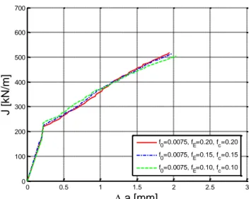
The parameters fc and fE, controlling the extinction of the cell element, do not influence the JR-curve in any significant way if they are chosen from the interval 0.10-0.20, see Figure 0.3 and Figure 0.4. Values of fc lower than 0.10 do however influence the JR-curve, see Figure 0.4. Hence, the model predictions are not sensitive to the choice of values for fc and fE, as long as they are in the range 0.10-0.20.

Figure 0.3. Comparison of numerical JR-curves for models with varying fE and fc values.

Figure 0.4. Comparison of numerical JR-curves for models with varying fc values. The second step is to determine the fracture process parameters, this procedure is described in more detail in [5]. The fracture process parameters f0 and D are the main parameters controlling the crack growth resistance behavior, in shear stress states with near zero triaxiality k also plays a significant role. To successfully

determine these parameters, experimental data describing the crack growth behavior and the behavior in pure shear is needed. An experimentally generated JR -curve is a suitable candidate for this purpose together with results from a shear test.

D can be determined from the crack tip opening displacement (CTOD) at initiation.

CTOD scales with the near tip deformation and is also a relevant measure of the size of the fracture process zone. To take D as the CTOD at initiation is therefore suitable. CTOD at crack initiation or D can be determined from JIc with the relation

y Ic

J

d

D





where JIc is the J-value at initiation of crack growth, σy is the yield strength and d is a non-dimensional constant ranging from 0.30 to 0.60 depending on the material

0 0.5 1 1.5 2 2.5 3 0 100 200 300 400 500 600 700  a [mm] J [kN /m ] f₀=0.0075, f_E=0.20, f_c=0.20 f₀=0.0075, f_E=0.15, f_c=0.15 f₀=0.0075, f_E=0.10, f_c=0.10 0 0.5 1 1.5 2 2.5 3 0 100 200 300 400 500 600 700 da [mm] J [kN /m ] f₀=0.008, f_E=0.20, f_c=0.20 f₀=0.008, f_E=0.20, f_c=0.15 f₀=0.008, f_E=0.20, f_c=0.10 f₀=0.008, f_E=0.20, f_c=0.05

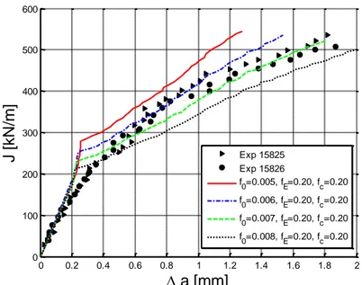
strain hardening and yield strength [14]. The initial void volume fraction f0 can be determined from matching the cell model to the experimentally generated JR-curve. And finally, the shear damage coefficient k is determined by matching the experimental results from a shear test to the predicted results from a FE-model. Below in Figure 0.5 the influence of f0 on the JR-curve is illustrated and in Figure 0.6 the influence of k on the predicted load deformation curve of a shear test is compared to experimental results.

Figure 0.5. Effect of varying initial void volume fraction, f0, on the JR-curve.

Figure 0.6. Influence of values of k on the predicted load deformation curve.

In order to generate a JR-curve from the numerical results of the cell model, the location of the crack front needs to be defined. In all analyses in this report, the crack front is defined by the line connecting locations at the crack plane where

f=0.1. At f=0.1 a cell element has lost most of its load carrying capacity.

Furthermore, the J-integral needs to be calculated.

0 0.2 0.4 0.6 0.8 1 1.2 1.4 1.6 1.8 2 0 100 200 300 400 500 600  a [mm] J [kN /m ] Exp 15825 Exp 15826 f₀=0.005, f_E=0.20, f_c=0.20 f₀=0.006, f_E=0.20, f_c=0.20 f₀=0.007, f_E=0.20, f_c=0.20 f₀=0.008, f_E=0.20, f_c=0.20 0 1 2 3 4 5 6 0 1 2 3 4 5 6 Deformation [mm] L o a d [ kN ] FEM k_w=1.5 FEM k_w=1.7 Experimental results Experimental results

3 Experimental program

All the experiments were conducted at the department of Solid Mechanics at the Royal Institute of Technology (KTH). The experiments were done to obtain the characteristics of the material in pure shear conditions, to be able to determine the kw parameter in the shear modified Gurson model. Complementary experiments to the experimental program carried out in the work by Bolinder [3] were also conducted. The experimental program detailed in [3] looked at the influence of load history on material fracture toughness. The complementary experiments were done to give a more complete picture of the effect of load history on the material fracture toughness. The experiments in [3] where motivated from earlier experiments by Bolinder et al. [2], which looked at the effect of residual stress fields on the fracture toughness.

In the experimental program, it was decided to look at one material, A533B-1. This is the same material which had been used in [3] and [2], thus there was no need to perform standard uniaxial tensile tests or cyclic tests, since these tests had already been conducted and the test data was available. The stress-strain curve of the material A533B-1 is shown in Figure 0.7.

Figure 0.7. Stress-strain curve of material A533B-1 at room temperature.

The shear tests were conducted using modified Iosipescu tests. The specimen geometry is shown in Figure 0.8. For a more detailed description of the tests, see Chapter 3.1 below.

For the experiments, examining the effect of load history, specimens subjected to different levels of compression or tension were used. To look at the isolated effect of the load history, the pre-loading of the material was done so it would not introduce any residual stresses, this is described below. After the materials had been pre-loaded, 3PB specimens with side groves were manufactured from these materials. These test specimens were then used in standard J-R tests to determine

0 0.1 0.2 0.3 0.4 0.5 0.6 0.7 0.8 0.9 1 0 200 400 600 800 1000 1200

True strain

T

ru

e

st

re

ss

[M

P

a

]

the JIc values. The specimen geometry is shown in Figure 0.9. The test program is outlined below.

 Shear tests, two modified iosipescu specimens

- Material: A533B-1

- Geometry: W= 20 mm, B= 2 mm, S=4W, l=1.7, h=6.8,

Angle 1=35°, Angle 2=55°

- Testing: modified Iosipescu shear test

 Material pre-loaded in compression, two specimens

- Material: A533B-1

- Level of pre-load: 4.5% total strain

- Geometry: W= 27 mm, B=W/2, S=4W, a=0.5W

- Testing: J-R tests in 3PB

 Material pre-loaded in tension, four specimens

- Material: A533B-1

- Level of pre-load: 4.5% or 8% total strain

- Geometry: W= 27 mm, B=W/2, S=4W, a=0.5W

- Testing: J-R tests in 3PB

Figure 0.8. Base geometry of modified iosipescu test specimen.

h

Angle 1

_{Angle 2}

W

Angle 2

l

S

Figure 0.9. Base geometry of the 3PB specimens.

Shear test

3.1

The shear tests were all performed at the department of Solid Mechanics at KTH using a shear rig, see Figure 0.10. During the test piston, load data and also the movement of the rig were recorded.

Figure 0.10. Test rig used for the shear test.

The loading of the specimen in this rig leads to a pure shear load with near zero triaxiality and the -measure equal to unity.

Pre-Loading

3.2

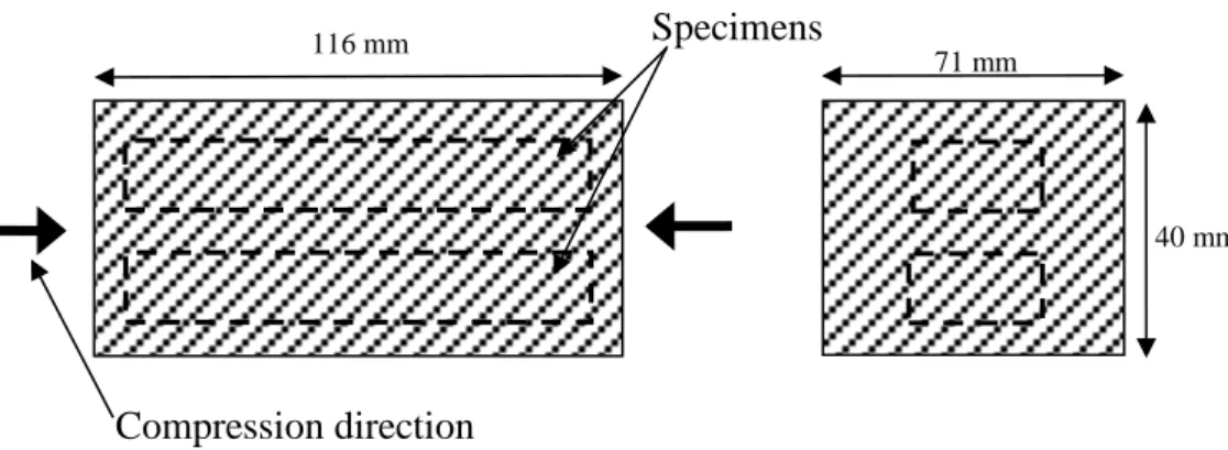
Pre-loading of the material was conducted at two different levels of pre-strain in tension and at one level of pre-strain in compression. For the material pre-loaded in compression, one rectangular piece of the material was machined. This piece was then loaded at room temperature to a maximum total strain of 4.5%. From the rectangular loaded piece the test specimens were then machined. Figure 0.11 shows the dimension and the orientation of the test specimens.

S

a

W

Figure 0.11. Dimensions of material pre-loaded in compression.

For the material pre-loaded in tension, two cylindrical pieces were machined. These cylindrical rods were threaded in the end for mounting in the testing rig. These two pieces were then loaded in tension at room temperature to a maximum total strain of 4.5% or of 8.0%. From each rod, two specimens were machined, as Figure 0.12 shows.

Figure 0.12. Dimensions of material pre-loaded in tension.

Fracture testing

3.3

The fracture tests were conducted as standard J-R testing according to ASTM E 1820 [15]. All specimens were loaded in 3PB during the fracture testing. The load, CMOD and LLD (Load Line Displacement) data were recorded during the tests. The crack growth was monitored with compliance calculations. The tests were ended with a fatigue loading in order to obtain two different crack fronts on the crack surface. The first front is the initial crack depth and the second is the fatigue front at the end of the testing. After the fracture testing was finished, the specimen was broken up to show the crack surfaces, and also to measure the different crack fronts. 116 mm 71 mm 40 mm

Compression direction

Specimens

300 mm

35 mm

Loading direction

Specimens

4 Experimental Results and discussion

Shear tests

4.1

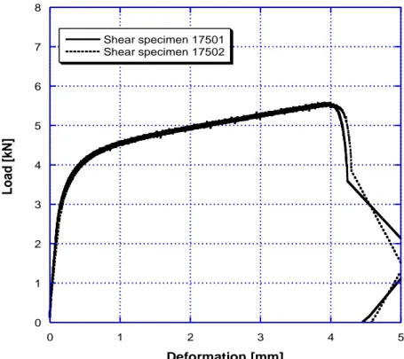
Figure 0.13 below shows the load-deformation results for the isopescu tests.

0 1 2 3 4 5 6 7 8 0 1 2 3 4 5 Shear specimen 17501 Shear specimen 17502 Loa d [k N ] Deformation [mm]

Figure 0.13. Load-deformation curves from iosipescu test.

Fracture tests

4.2

Figure 0.14 below shows the load-CMOD (Crack Mouth Opening Displacement) curves of the performed fractures tests together with earlier results from [3] without pre-load. The curves are shown without the unloadings for clarity. For Figure 0.14 the red color corresponds to a pre-load of 8% total strain, green color corresponds to 4.5% total strain and black corresponds to no pre-load.

Figure 0.14. Experimental load-CMOD curves for (a) specimens pre-loaded in compression and (b) specimens pre-loaded in tension.

From the load-CMOD curves, a clear effect of the pre-loading of the material can be seen for all levels of pre-load. The results also indicate that the pre-loaded specimens start to plastically deform earlier than the virgin material. One explanation to the trend seen in Figure 0.14 is the Bauschinger effect. The global moment gives rise to both compressive and tensile stresses over the ligament of the specimen. In the case where the specimens were pre-loaded in compression, the tensile part of the stresses over the ligament will lead to earlier plasticity than what would be the case for a virgin material and vice versa for the material pre-loaded in tension. This can also be understood by the hysteresis loop from a cyclic test of the

0 0.25 0.5 0.75 1 1.25 1.5 0 2 4 6 8 10 12 14 16 18 20

CMOD [mm]

P

[

kN

]

CMOD [mm]

P

[

kN

]

(b)

(a)

material shown below in Figure 0.15. The reversed stresses with regard to the pre-load will give rise to plasticity at a lower stress magnitude. From the hysteresis loop from a cyclic test in Figure 0.15 it is evident that the material experiences the Bauschinger effect.

Figure 0.15. Cyclic test data for A533B-1.

The J-R test results from all the tests and earlier results from [3] without pre-load are presented below in Figure 0.16, Figure 0.17 and Table 0.1. Figure 0.16 shows all the results for specimens pre-loaded in compression and without pre-load, while Figure 0.17 shows results for specimens loaded in tension and without pre-load. For both Figure 0.16 and Figure 0.17 the red color corresponds to a pre-load of 8% total strain, green color corresponds to 4.5% total strain and black corresponds to no pre-load. In table 4.1 earlier results from [3] are included for comparison and to get a more complete picture. Average values of the JIc data presented in Table 4.1 are also plotted in Figure 4.6.

Engineering strain [%]

Stress

-100 0 100 200 300 400 500 600 0 0.5 1 1.5 2 No pre-load No pre-load 4.5% compression 4.5% compression

J

[k

N

/m]



a [mm]

Figure 0.16.

J-integral results versus crack growth, with and without

compressive pre-load.

J

[k

N

/m]



a [mm]

Figure 0.17.

J-integral results versus crack growth, with and without tensile

pre-load.

Table 0.1. JIc values for all the test specimens. Total strain

[%]

JIc for specimens pre-loaded in compression [kN/m]

JIc for specimens pre-loaded in tension [kN/m] 0 249 262 249 262 1.5 249 235 270 279 3.0 256 220 248 238 4.5 218 209 188 179 6.0 170 163 137 152 8.0 - - 129 166 100 150 200 250 300 0 1 2 3 4 5 6 7 8 Pre-loaded in compression Pre-loaded in tension J Ic [ k N /m ] Pre-strain [%]

Figure 0.6. Effect from pre-load on material initiation fracture toughness.

From the results above, it is clear that for specimens pre-loaded to 8% and to 6 % total strain, large effects from the pre-loading of the material are seen. For specimens pre-loaded to 4.5 % total strain, an effect can also be seen, but not as large as for those pre-loaded to 6% and to 8%. The effect from pre-loading can be seen for both pre-loading in tension and compression, but the effect is larger for the specimens pre-loaded in tension. It can also be concluded that no distinctive influence on crack initiation is observed from pre-loadings to 1.5 or to 3 %. The reason for the large difference in the observed change in material fracture toughness from a pre-load of 6% or 8% and not 1.5% or 3% total strain is partly due to the kinematic hardening of the material, but also for the material pre-loaded in tension due to debonding of inclusions during the pre-load. This was observed in a metallurgical examination of the pre-loaded material, see Figure 4.7 below. This also explains the difference in the seen effect between pre-loading in compression compared with pre-loading in tension.

Figure 4.7. Metallurgical examination to investigate the effect on inclusions from pre-straining; (a) material pre-strained in tension to 6% total strain, (b) material pre-strained in compression to 6% total strain.

Earlier experimental work by Sivaprasad et al. [16] on HSLA steels have shown similar trends. Their results showed that for pre-loads up to 2 % no effect on the fracture toughness was seen. At greater pre-load levels their results showed a decrease in fracture toughness in almost direct proportion to the amount of pre-load. Experimental results on 316 stainless steel and 4340 steel presented by Liaw and Landes [17] showed a decrease in fracture toughness regardless of the level of pre-load.

It should be noted that the effects seen as a result of work hardening are due to a prior pre-load at room temperature. Hence, these effects are not representable for cases were the material exhibits a level of pre-strain caused by welding.

5 Predictions using Cell Modelling

In this chapter predictions of experimental results described in [2], will be done by the use of micromechanical modeling. This is done by the use of a cell model. With the cell model the growth and coalescence of voids and the interaction between the fracture process zone and the background material is modeled. The cell model parameters will be determined from experimental results of a uniaxial tensile test, from a standard fracture test on 3PB specimen and from a shear test using a modified iosipescu test specimen. Subsequently the cell modeling technique will be used with the determined material parameters in predicting the experimental results. The predictions show the capability of the cell modeling technique employed in describing the effects from a residual stress field. The numerical computations with the finite element method were executed with ABAQUS explicit [11].

In order to generate JR-curves from the numerical results of the cell models the J-integral needed to be calculated. For calculating the J-J-integral a different method other than the method described in ASTM E 1820 [15] was used. The reason for using the non-standard routine was that the standard method according to ASTM E 1820 [15] will not give reliable data at low load levels for the specimens with residual stresses described in [2], since it does not take into account the elastic contribution from the residual stresses to the J-integral. An alternative method using FE-analyses was previously developed by Bolinder et al. in [2], for a non-standard specimen with and without residual stresses. This method was also used in this study for evaluating the J-integral from the numerical results of the cell model. In the method a correlation between the J-integral and CMOD is obtained by using several FE-models. With this correlation the J-integral is obtained from the CMOD results, in Figure 0.18 an example of the J-CMOD curves is shown. For a thorough description of the method the reader is referred to [2]. The reason for using this method in evaluating the J-integral from the numerical results is to give an accurate comparison with the experimental results in [2].

Figure 0.18. Example of J-CMOD curves used in evaluating the J-integral from the experiments.

x 102

FE-models

5.1

5.1.1 Shear specimen

A script was written by using the Python code in order to create a parameterized FE-model for ABAQUS. With this script it was possible to create a model of the iosipescu test specimen. The script makes it possible to change all the geometric entities and also the refinement of the element mesh. The scripted model was used to evaluate and test different geometries of the specimen. Furthermore, a sensitivity analysis of the element mesh was conducted. The sensitivity analysis led to the final mesh setup illustrated below in Figure 0.19. The element size in the refined region or damage zone was 100x100x250 m with 250 mm in the vertical direction of the specimen. This was a sufficiently refined mesh in the damage zone to correctly capture the shear localization. The element used in all analyses was the 8-node linear brick element with reduced integration and hourglass control (C3D8R). The final geometry of the test specimens used in the analyses is the same as the one used in the experiments, as given in Chapter 3.

5.1.2 Fracture specimen

A script was written by using the Python code language in order to create a parameterized FE-model for ABAQUS. With this script it is possible to model a 3PB specimen with and without side grows and also with and without a notch. The geometries of the test specimens are shown in Figure 0.20 where W=27 mm.

Figure 0.20. Base geometry of (a) standard 3PB specimen with side-grooves and (b) notched test specimen [2].

With the script it is possible to control the cell element layer in great detail. During the course of the work several FE-models were created with different setups of the element mesh. These were used in sensitivity analyses which led to the final element mesh setup described below. Due to symmetry, only a quarter of the test specimens were modeled. Figure 0.21 shows the two different FE-models used in the following analyses.

a

R

_L

l

S

W

Geometry:

B=0.5W

B

=x

L=5W

S=4W

R=0.25W

l1=0.2W

a=0.35W

S

L

W

a

Thickness

B, B

Thickness B

(a)

_(b)

Figure 0.21. Three dimensional finite element mesh for (a) a quarter model of the side-grooved three point bending specimen, (b) a quarter model of the un-grooved notched three point bending specimen.

The fracture process zone or the cell element layer is shown in Figure 0.22. The cell elements were modeled with the height and length of D/2. The value of D and how it is determined is explained in Chapter 5.2.

Figure 0.22. The arrangement of the void containing cells and the surrounding region.

The depth of the cell elements were varied with the position relative to the free surface with larger element depths near the center symmetry surface and with smaller depths near the free surface. At the free surface the element depth was equal to D/2. Both FE-models were meshed with a total of 20 element layers through the thickness. Figure 0.23 shows the element mesh trough the thickness. A thorough study of the influence of element thickness is presented by Qian in [18] and this study was decisive in deciding the element layer setup. Both models used in the analyses were meshed with 8-node linear brick element with reduced integration and hourglass control (C3D8R).

Figure 0.23. The arrangement of the finite element meshes through the thickness used in both FE-models.

Determining the cell model parameters

5.2

The matrix material behavior of the material model was modeled as elastic multi-linear plastic with isotropic hardening. The material parameters for the matrix material are given below in Table 0.2.

Table 0.2.

Matrix material parameters used in the FE-model for material

A533B-1.

The micromechanical parameters q1 and q2 strongly depend on the material stress-strain relation. For this report q1 and q2 were determined from the correlations to σ0 and N derived by Faleskog et al. in [13]. To be able to determine the parameters q1 and q2 the uniaxial tensile test result was fitted to a power law curve on the form,

. 0 / 1 0 0 0 0





















The values for σ0 and N were then used to determine q1 and q2 from the tabulated values in [13].

Figure 0.24 below shows the stress-strain curve and the power law fit.

Figure 0.24. Stress-strain curve with power law fit for material A533B-1.

The values of the void volume fractions fc and fE are typically chosen from the interval 0.10 to 0.20. The model predictions are rather insensitive to the choice of fc and fE as long as their values are in the interval mentioned above. The results in Figure 0.4 show a slightly more curved JR-curve for values of fc and fE set to 0.10 and 0.20 respectively as compared to values of fc and fE both set to 0.20. This was considered when choosing values for fc and fE. In the following models fc and fE were therefore set to 0.10 and 0.20 respectively. Table 0.3 below presents the micromechanics parameters used in the models of this study.

Table 0.3. Micromechanics parameters used in the material model. Micromechanics q1 1.7046 q2 0.8503 fE 0.20 fc 0.10 0 0.1 0.2 0.3 0.4 0.5 0.6 0.7 0.8 0.9 1 0 200 400 600 800 1000 1200

True strain

T

ru

e

st

re

ss

[M

P

a

]

Bridgman corected experimental results

Power law hardening N=0.15 ₀=360 MPa

Data points used for power law fit FEM

The fracture process parameters f0 and D are the parameters primarily controlling the crack growth resistance behavior. These are hence decided from an experimentally determined Jr-curve using a standard specimen. The JIc value was determined from the Jr-curve in Figure 0.25, which led to a D of 0.250 mm by using Equation 4.

Figure 0.25. Experimental JR-curve for side-grooved three point bend specimen without any prior preload.

The initial porosity f0 was decided by matching the cell model predictions to the experimental JR-curve see Figure 0.26. From these results the value determined for

f0 was 0.0070. In Figure 0.26 the load-CMOD curve from the experiment is also compared with the results from the FE-model and as can be seen it shows a good agreement between the FE-model and the experimental results.

(a) (b)

Figure 0.26.(a) Predicted JR -curves with varying f0 values compared with the experimental data for side-grooved three point bend specimen without any prior preload, (b) predicted load-CMOD curves with varying f0 valuescompared with the experimental load-CMOD curve for side-grooved three point bend specimen without any prior preload.

0 0.5 1 1.5 2 2.5 0 100 200 300 400 500 600 a [mm] J [kN /m ] Exp 15825 Exp 15826 f 0=0.0060, fE=0.20, fc=0.10 f₀=0.0070, f_E=0.20, f_c=0.10 f₀=0.0080, f_E=0.20, f_c=0.10 0 0.5 1 1.5 2 2.5 0 2 4 6 8 10 12 14 16 18 CMOD [mm] F [ kN ] Exp 15825 Exp 15826 f 0=0.0060, fE=0.20, fc=0.10 f 0=0.0070, fE=0.20, fc=0.10 f 0=0.0080, fE=0.20, fc=0.10

Finally the shear damage coefficient 𝑘

is determined by matching the

predicted results with the obtained experimental results, see Figure 0.27.

From the results below the value determined for 𝑘

is 1.58.

Figure 0.27. Predicted Load-Deformation-curve compared with the experimental data for two modified iosipescu test specimens.

Table 0.4 presents the fracture process parameters used in ABAQUS [11]

for the material model.

Table 0.4. Fracture process parameters used in the material model. Fracture process D [mm] 0.250 f0 0.0070 k 1.58 0 1 2 3 4 5 6 0 1 2 3 4 5 6

Deformation [mm]

L

o

a

d

[

kN

]

Evaluation of the capability of the cell modeling technique

5.3

in capturing the effects of residual stresses

In this chapter the capability of the cell modeling technique with the modified Gurson model in capturing the effects of residual stresses is evaluated. The ability to capture the effect of constraint is also shown since the specimens used in [2] had a non-standard geometry with a shallow crack which leads to lower constraint as compared to the standard specimen geometry used in determining the cell model parameter values. The cell model parameter values determined in chapter 5.2 will be used in all the analyses described below.

In [2] the residual stresses were introduced by pre-loading a notched test specimen, see Figure 0.28. The pre-load leads to a stress concentration at the notch with compressive stresses normal to the crack surface. When the specimen is unloaded, a residual stress field is introduced due to the plastic deformations during the pre-load. The resulting residual stresses are tensile at the notch since they were compressive during the pre-load. For a more thorough description of the residual stress field and how it is introduced, see [2].

Figure 0.28. In-plane compression of the notched test specimen.

To correctly model the introduction of the residual stress field a separate FE-model was used. The reason for this was the modeled crack tip notch in the FE-model with cell elements. The modeled crack tip notch introduces a stress concentration when the specimen is pre-loaded in compression. In the experimental specimens the crack tip is sharp and no stress concentration is introduced at the crack tip during pre-loading. Hence, the crack tip notch would lead to an undesired stress concentration not present in the test specimens. Therefore a separate FE-model was used in obtaining a correct residual stress field. In the FE-model an element layer was introduced at the crack surface during the pre-load, see Figure 0.29, which was removed after unloading of the specimen.

Figure 0.29. Introduced element layer during compressive pre-load.

The stress and strain results from the FE-model without cell elements were then used as pre-scribed initial conditions for the FE-model with cell elements. The resulting residual stress field in the cell element model was compared with the residual stresses in the FE-model without cell elements to verify the procedure of

introducing the residual stresses, see Figure 0.30. As can be seen in Figure 0.30, the residual stress field agrees well between the two models, leading to a confidence in the correctness of the procedure of introducing the residual stress field.

-4 108 -2 108 0 2 108 4 108 6 108 8 108 1 109 1.2 109 0 0.2 0.4 0.6 0.8 1 Cell model Compresive model  yy [ M P a] x/(W-a)

Figure 0.30. Comparison of opening stress along the ligament in front of the crack tip.

Two FE-models were used in the analyses, one with and one without residual stresses, in order to mimic the experimental set-up in [2]. The predicted load-CMOD curves are compared to the experimental results in Figure 0.31. Figure 0.31 shows a very good agreement between the predicted and experimental results, leading to a confidence in the correctness of the model.

Figure 0.31. Predicted load-CMOD curves as compared with the experimental load-CMOD curves for un-grooved notched three point bend specimen, (a) without residual stresses, (b) with residual stresses.

In Figure 0.32 below the predicted JR-curves from the two FE-models with and without residual stresses are compared to the experimental results from [2]. The experimental results show a visible scatter at larger amount of crack growth. The predicted results lie within the scatter range of the experimental results. Further, as for the experimental results, no significant effect from the residual stress field can be seen on crack initiation for the predicted results. Hence, it can be concluded that

0 0.5 1 1.5 2 2.5 0 5 10 15 20 25 30 CMOD [mm] P [ kN ] Specimen 15297 no pre-load Specimen 15298 no pre-load Specimen 15300 no pre-load Numerical prediction no pre-load

0 0.5 1 1.5 2 2.5 0 5 10 15 20 25 30 CMOD [mm] L r [P /P L ] Specimen 15291 pre-load Specimen 15295 pre-load Specimen 15299 pre-load Numerical prediction pre-load

the cell model with the shear modified Gurson model handles the effect from residual stresses correctly with regard to crack initiation and crack growth. These results show the capability of the cell modeling technique with the shear modified Gurson model in capturing the effect from residual stresses. The results in Figure 0.32 also show the capability of the cell modeling technique in capturing the increased fracture toughness for the non-standard specimen, caused by constraint effects, compared to the standard specimen.

Figure 0.32. Predicted JR -curves with and without residual stresses compared with the experimental data for un-grooved notched three point bend specimens with and without residual stresses.

Figure 0.33 shows a comparison between the prior results from [3] using the Gurson model incorporated in ABAQUS and the results using the shear modified Gurson model. As can be seen from Figure 0.33, the previous work predicted results that lie on the upper bound of the scatter. The reason for the upper bound prediction in [3] can be explained by the low triaxiality at the free surface of the specimens. The Gurson material model used in [3] underestimates the void growth at low stress triaxiality. Hence, the model prediction overestimates the material tearing resistance at the free surface. This effect increases as the crack tunneling becomes more severe as the load increases, hence leading to an overestimated tearing resistance at larger amounts of crack growth. The overestimated tearing resistance seen in the predictions in [3] can be rectified by using the shear modified Gurson model, as can also be seen in Figure 0.33. The shear modified Gurson model, as discussed earlier, does take in to account the void growth at low triaxiality and for shear dominated states. An improvement in the predictions can be seen by using the shear modified Gurson model.

0 0.2 0.4 0.6 0.8 1 1.2 1.4 1.6 1.8 2 2.2 0 100 200 300 400 500 600 700 800 900 1000 a [mm] J [kN /m ]

Experimental results no pre-load (fit) Experimental results pre-load (fit)

Experimental results no pre-load (color marking) Experimental results pre-load (color marking) Prediction no pre-load (fit)

Prediction pre-load (fit) Blunting line

Figure 0.33. Predicted JR -curves with and without residual stresses as compared with the experimental data for un-grooved notched three point bend specimens with and without residual stresses. (a) Prediction with standard Gurson model and (b) prediction with shear modified Gurson model.

In Figure 0.34 the predicted J-integral against Lr for specimens with and without residual stresses are compared to the experimental results. The predicted results show a very good agreement with the experimental results. Recreating the seen effect from the residual stresses on the J-integral at low loads also show the diminishing effect as the load increases.

Figure 0.34. Predicted J values versus Lr results compared to experimentally obtained J values versus Lr results for un-grooved notched three point bend specimen with and without residual stresses.

0 0.2 0.4 0.6 0.8 1 1.2 1.4 1.6 1.8 2 2.2 0 100 200 300 400 500 600 700 800 900 1000 a [mm] J [kN /m ]

Experimental results no pre-load (fit) Experimental results pre-load (fit) Experimental results no pre-load (color marking) Experimental results pre-load (color marking) Prediction no pre-load (fit) Prediction pre-load (fit) Blunting line 0 0.2 0.4 0.6 0.8 1 1.2 1.4 1.6 1.8 2 2.2 0 100 200 300 400 500 600 700 800 900 1000 a [mm] J [kN /m ]

Experimental results no pre-load (fit) Experimental results pre-load (fit) Experimental results no pre-load (color marking) Experimental results pre-load (color marking) Prediction no pre-load (fit) Prediction pre-load (fit) Blunting line 0.2 0.3 0.4 0.5 0.6 0.7 0.8 0.9 1 1.1 1.2 0 100 200 300 400 500 600 Lr [P/P L] J [kN /m ] Specimen 15291 pre-load Specimen 15292 pre-load Specimen 15293 pre-load Specimen 15295 pre-load Specimen 15299 pre-load Specimen 15297 no pre-load Specimen 15298 no pre-load Specimen 15300 no pre-load Numerical prediction no pre-load Numerical prediction pre-load

6 Discussion

From the experimentally evaluated JR-curves, a large effect on the material fracture toughness is seen for specimens pre-loaded to 8% total strain. An effect from the pre-load is also seen for the specimens pre-loaded to 4.5% total strain. This holds for pre-loading in both tension and compression but the effect is larger in the specimens pre-loaded in tension. These results fit well with the earlier results from [3]. It should be noted that the effects seen, as a result of work hardening, are due to a prior pre-load at room temperature. Hence, these effects are not representative for cases were the material exhibits a level of pre-strain caused by welding.

A difference in the effect on the fracture toughness between specimens pre-loaded in tension and compression is seen in the experiments carried out in this study and in the prior work [3]. This observed difference can be explained by debonding of large inclusions during the pre-load in tension. This was observed in a metallurgical examination of the pre-loaded material, see Figure 4.6. Where debonding of the large inclusion is seen for material pre-loaded in tension but not for material pre-loaded in compression.

The computational work done in Chapter 5.3 have shown numerical predictions of cracked geometries, other than the specimen geometry used in determining the material parameters, give good results using the same determined material parameter values. Hence, the scheme outlined by Faleskog et al. [13] and Gao et al. [5] to determine the material parameters based on a uniaxial tensile test, a standard fracture test and a shear test is shown to be a structured and sound approach. The cell model captures the effects attributable to residual stresses, as seen in the experimental work by Bolinder et al. [2]. From the predicted results presented in Chapter 5.3 the same conclusions that were made from the experimental results in [2] can be drawn with regard to fracture toughness and the decreasing influence on the J-integral for increasing primary load. The predictions made here also show an improvement as compared to earlier predictions in [3]. The predicted JR-curves for the non-standard specimens with and without residual stresses lie within the scatter range of the experimental results. The Gurson material model used in [3] underestimated the void growth at low stress triaxiality. Hence tearing resistance of the material was overestimated. This is resolved in this study by use of the shear modified Gurson model, which takes into account void growth at low triaxiality and for shear dominated states.

This study describes the capability of the cell model in capturing the effects on ductile tearing from limited pre-load levels and a residual stress field.

7 Conclusions

From the numerical and experimental results presented in this study it can be concluded that:

 For specimens pre-loaded (work hardened) to 8% of total strain at room temperature in both tension and compression large effects are seen on both the tearing resistance and crack initiation. An effect from the pre-load is also seen for the specimens pre-loaded to 4.5% total strain. This holds for pre-loading in both tension and compression. Note though that the effect on the fracture toughness is greater in the specimens pre-loaded in tension.

 The shear modified Gurson model does capture the effects attributable to residual stresses, seen in the experimental work by Bolinder et al. [2], with regard to fracture toughness and the decreasing influence on the J-integral for increasing primary load.

 The shear modified Gurson model does not overestimate the fracture resistance, as was seen for the standard Gurson model.

 The results in Figure 0.32 also show the capability of the shear modified Gurson model for capturing the increased fracture toughness as compared to the standard specimen, which is due to the constraint effect.

8 Future work

There is the ambition to complement the modified Gurson model with the option to use kinematic material hardening. To be able to use kinematic hardening could possibly make it possible to correctly predict the seen effect on the JR-curves caused by the high pre-load levels.

Further in the future it is the ambition to use the modified Gurson model in studying the effect of residual stresses on ductile tearing at low primary load, specifically to study the effect on the residual stresses from a limited and stable crack growth.

The Gurson model could also be used in designing experiments, to avoid undesired and unpredictable test results and to be certain that the experiments give relevant results.

Other potential uses of the modified Gurson model could be to examine the size effects when using small fracture test specimens and also to examine the possibility to incorporate the ability to predict irradiation effects.

REFERENCES

[1] K. Nahshon and J.W. Hutchinson, "Modification of the Gurson Model

for shear failure," European Journal of Mechanics A/Solids, vol. 27, pp.

1-17, 2008.

[2] T. Bolinder and I. Sattari-Far, "Experimental evaluation of influence

from residual stresses on crack initiation and ductile crack growth at

high primary loads," Swedish Radiation Safety Authority, Report

number 2011:19, 2011.

[3] T. Bolinder, "Numerical simulation of ductile crack growth in residual

stress fields," Swedish Radiation Safety Authority, Report number

2014:28, 2014.

[4] P. Dillström, M. Andersson, I. Sattari-Far, and W. Zhang, "Analysis

strategy for fracture assessment of defects in ductile material," Swedish

Radiation Safety Authority, Report number 2009:27, 2009.

[5] X. Gao, J. Faleskog, and C.F. Shih, "Cell model for nonlinear fracture

analysis – II. Fracture-process calibration and verification,"

International Journal of Fracture, vol. 89, pp. 375-398, 1998.

[6] X. Gao, J. Faleskog, and C.F. Shih, "Ductile tearing in part-through

cracks: experiments and cell model predictions," Engineering Fracture

Mechanics, vol. 59, no. 6, pp. 761-777.

[7] L. Xia and C.F. Shih, "Ductile crack growth - I. A numerical study

using coputational cells with a microstructurally-based length scale,"

Journal of the Mechanics and Physics of Solids, vol. 43, pp. 233-259,

1995.

[8] L. Xia and C.F. Shih, "Ductile crack growth - II. Void nucleation and

geometry effects on microscopic fracture behavior," Journal of the

Mechanics and Physics of Solids, vol. 43, pp. 1953-1981, 1995.

[9] A.L. Gurson, "Continuum theory of ductile rupture by void nucleation

an growth: Part I – Yield criteria and flow rules for porous ductile

media," Journal of Engineering Materials and Technology, vol. 99, pp.

2-15, 1977.

[10] V. Tvergaard, "Material failure by void growth to coalescence,"

Advances in applied Mechanics, no. 27, pp. 83-151, 1990.

[11] Hibbit, Karlsson, and Sorenson, ABAQUS user manual.: Dassault

Systèmes.

[12] V. Tvergaard and A. Needleman, "Analysis of cup-cone fracture in a

round tensile bar.," Acta Metallurgica, vol. 32, pp. 157-169, 1984.

[13] J. Faleskog, X. Gao, and C.F. Shih, "Cell model for nonlinear fracture

analysis – I. Micromechanics calibration," International Journal of

Fracture, vol. 89, pp. 355-373, 1998.

[14] C.F. Shih, "Relationship between the J-integral and the crack opening

displacement for stationary and extending cracks," Journal of the

Mechanics and Physics of Solids, vol. 29, pp. 305-326, 1981.

[15] "Standard test method of measurement of fracture toughness," ASTM,

E 1820,.

[16] S. Sivaprasad, S. Tarafder, V.R. Ranganath, and K.K. Ray, "Effect of

prestrain on fracture toughness of HSLA steels," Material Science and

Engineering, vol. A284, pp. 195-201, 2000.

[17] P.K. Liaw and J.D. Landes, "Influence of prestrain history on fracture

toughness properties of steels," Metallurgical Transactions A, vol. 17,

pp. 473-489, 1986.

[18] X. Qian, "An out-of-plane length scale for ductile crack extensions in

3-D SSY model for X65 pipeline materials," International Journal of

Fracture, vol. 167, pp. 249-265, 2011.

Strålsäkerhetsmyndigheten Swedish Radiation Safety Authority

SE-171 16 Stockholm Tel: +46 8 799 40 00 E-mail: registrator@ssm.se Solna strandväg 96 Fax: +46 8 799 40 10 Web: stralsakerhetsmyndigheten.se

2015:53 The Swedish Radiation Safety Authority has a comprehensive responsibility to ensure that society is safe from the effects of radiation. The Authority works to achieve radiation safety in a number of areas: nuclear power, medical care as well as commercial products and services. The Authority also works to achieve protection from natural radiation and to increase the level of radiation safety internationally.

The Swedish Radiation Safety Authority works proactively and preventively to protect people and the environment from the harmful effects of radiation, now and in the future. The Authority issues regulations and supervises compliance, while also supporting research, providing training and information, and issuing advice. Often, activities involving radiation require licences issued by the Authority. The Swedish Radiation Safety Authority maintains emergency preparedness around the clock with the aim of limiting the aftermath of radiation accidents and the unintentional spreading of radioactive substances. The Authority participates in international co-operation in order to promote radiation safety and finances projects aiming to raise the level of radiation safety in certain Eastern European countries.

The Authority reports to the Ministry of the Environment and has around 300 employees with competencies in the fields of engineering, natural and behavioural sciences, law, economics and communications. We have received quality, environmental and working environment certification.