2017:25 Evaluation of weld fatigue reduction in austenitic stainless steel pipe components

(1)

Research

Evaluation of weld fatigue reduction

in austenitic stainless steel pipe

components

2017:25

Authors: Dave Hannes

Magnus Dahlberg Thomas Svensson Andreas Anderson

(2)

(3)

SSM perspective

Background

The performed investigation is a continuation of the work performed in SSM 2015:38 where fatigue tests were performed on pressurized welded austenitic stainless steel piping components. The specimens were sub-jected to a realistic variable amplitude loading with mainly reversed bend-ing deformation and particular focus on high cycle fatigue. The previous fatigue results were quite dependent on the estimation of the stress con-centration factor of the weld. Therefore, it was decided to continue this research by performing fatigue tests on pressurized non-welded austenitic stainless steel piping components.

Objective

The present study is aimed to investigate the margins of the ASME design curve for austenitic stainless steel, by performing fatigue experiments on a realistic non-welded austenitic stainless steel piping component and compare the results with the previous study where fatigue experiments on welded austenitic stainless steel piping components were performed. In this way, a more realistic analysis can be made of the fatigue strength reduction factor (FSRF).

Another objective has been to improve the knowledge on the

transferabil-ity for a non-welded piping component subjected to variable amplitude

loading by comparing with smooth specimen data obtained with constant amplitude fatigue testing.

Results

Extensive conservatism in the ASME approach to deal with transferability was confirmed. For the considered welded piping, the ASME design curve corresponded to a reduction in allowable number of cycles with a factor of at least 2.3. For the welded piping component, the fatigue strength reduc-tion factor FSRF was estimated to 1.8 by comparing the results from the welded and unwelded pipe experiments.

The work has increased the understanding of the ASME margins and has improved the knowledge on fatigue in austenitic stainless steel compo-nents and the fundamental issue of transferability.

Need for further research

There is a need to further verify the results of this study by performing more fatigue experiments on larger and thicker piping components and using other welding configurations. Also, there is a need to further investi-gate the complex material behavior of austenitic stainless steel be in order to better describe the strains at the weld toe or strain concentration. Project information

Contact person SSM: Björn Brickstad Reference: SSM2016-564

(4)

(5)

2017:25

Authors: Dave Hannes, Magnus Dahlberg 1)_{, Thomas Svensson}2)_{. Andreas Anderson}3)

1)_{Inspecta Technology AB, Stockholm, Sweden} 2)_{TS Ingenjörsstatistik, Borås, Sweden}

3)_{RISE Research Institutes of Sweden, Borås, Sweden}

Evaluation of weld fatigue reduction

in austenitic stainless steel pipe

(6)

This report concerns a study which has been conducted for the Swedish Radiation Safety Authority, SSM. The conclusions and view-points presented in the report are those of the author/authors and

(7)

Evaluation of weld fatigue reduction

in austenitic stainless steel pipe

components

Summary

The performed investigation is a continuation of the work performed in SSM 2015:38 and consists of fatigue tests on water pressurized non-welded austenitic stainless steel piping components. The specimens are subjected to a realistic variable amplitude loading with mainly reversed bending deformation and particular focus on HCF.

The experimental results allowed to determine a weld fatigue strength reduction factor (FSRF) for a similar piping component with circumferential butt weld in as-welded condition from SSM 2015:38. It was estimated to about 1.8. Both Basquin and Langer fatigue models were used and yielded consistent results. The weld FSRF did not exhibit any dependency on load level or number of load cycles and could thus be assumed to be constant. The experimental estimate of the FSRF highlighted the conservatism of the ASME approach based on stress indices.

The resulting margins in the fatigue design curve for austenitic stainless steel in ASME III were investigated. Extensive conservatism in the ASME approach to deal with transferability was confirmed. For the considered welded piping, the ASME design curve corresponded to a reduction in allowable number of cycles with a factor of at least 2.3. For the non-welded piping component, the fatigue life reduction factor was minimum 1.6. The ASME design curve represents thus a survival probability largely in excess of 95 % for the considered realistic components and loading configurations.

The experimental investigation resulted in increased understanding of the effect on the fatigue strength for piping components of a welding joint in as-welded condition. It improved the knowledge on the crucial issue of transferability and increased fundamental understanding for fatigue in piping components.

(8)

1 Nomenclature

A Factor in Langer equation

B Exponent in Langer equation

C Cut-off or asymptotic limit in Langer equation

E Young’s modulus

i Dummy index

k Scaling factor for strain amplitudes

Kf Fatigue strength reduction factor

Kt Concentration or notch factor

m Total number of strain cycles in a load sequence

n Total number of strain cycles in a load sequence with amplitudes exceeding the cut-off limit

N Total number of cycles, predicted or experimental fatigue life

NC Total number of load cycles with strain amplitudes exceeding the cut-off limit C

q Notch sensitivity factor

Rm Tensile strength

Rp0.2 Yield strength

t Nominal wall thickness

α Factor in Basquin equation

β Exponent in Basquin equation

ε Strain (axial)

ε0 Mean nominal strain (due to internal pressure)

εa Strain amplitude

εm Mean strain

σ Standard deviation of error of predicted logarithmic life

∎̂ Estimated quantity

∎max Maximum value

(10)

2 Introduction

2.1 Background

Rules for construction or design of nuclear facility components are specified in section III of the ASME Boiler and Pressure Vessel Code [1]. The design against fatigue is based on the use of prescribed material specific fatigue design curves (Wöhler diagrams). Such design curves correspond to at least 95% survival probability and are derived by adjustment of a mean curve. The mean curve is typically obtained by fitting to relatively large amounts of data from mainly laboratory experiments in air on small, smooth test specimens subjected to constant amplitude loading. The fatigue design curves are however intended for real components subjected to realistic loading. The adjustment of a mean curve therefore needs to account for the fundamental and challenging issue of transferability. It is essential in understanding and preventing fatigue in real or relevant components, but is affected by a large amount of variables [2]. The fatigue design curves in ASME III [1] are obtained by correcting the mean curve with adjustment factors on the strain (or stress) or the cycles, whichever is more conservative. The fatigue design curve in ASME III [1] for austenitic stainless steel (SS) is obtained from an adjustment of a mean curve derived by ANL [2]. The adjustment factor for strain (or stress) is equal to 2 and the one for the number of cycles equals 12. Prior to 2010, the latter adjustment factor equaled 20 and a revised version of [2] including new experimental data proposes to reduce the adjustment factor on the number of cycles to 10. The conservatism or margins of the fatigue design curves in ASME III [1] is thus closely related to the magnitude of these adjustment factors.

The fatigue design curves in ASME III [1] are to be used in conjunction with a local fictitious (elastic) stress amplitude. The local stress measure can be determined from a nominal stress and different stress indices defined in ASME III [1], which account for various effects related to geometry or loading. The stress concentration, i.e. when the local stress exceeds the nominal stress, will typically result in a local fatigue strength reduction of the component or structure. Following the definition in NB-3200 of ASME III [1], the fatigue strength reduction factor (FSRF) is a stress intensification factor which accounts for the effect of a local structural discontinuity (stress concentration) on the fatigue strength. Applying this definition to a welding joint yields that the FSRF for a given weld, material, component geometry and loading configuration is given by the ratio of the non-welded component’s fatigue strength and the fatigue strength of the same component with the considered welding joint. The assessment is performed for a given number of cycles. The FSRF is typically determined through experiments, but in the absence of experimental results the FSRF is often approximated by the stress concentration factor, i.e. the ratio of a local and a nominal stress measure. The latter being defined such that any effects of the local structural discontinuity are excluded, i.e. typically some distance away from the stress concentration. Welding joints typically represent a local structural discontinuity and the stress indices used in piping design specified in NB-3600 of [1] can be interpreted as a FSRF [3]. The FSRF increases with number of cycles and reaches a maximum value at the fatigue limit or high cycle fatigue (HCF) regime [3]. This maximum value is often used as a conservative design measure also applicable for low cycle fatigue (LCF). A reduction of the fatigue design curves with a FSRF allows their use in conjunction with a nominal stress measure.

(11)

2 Introduction

2.1 Background

Rules for construction or design of nuclear facility components are specified in section III of the ASME Boiler and Pressure Vessel Code [1]. The design against fatigue is based on the use of prescribed material specific fatigue design curves (Wöhler diagrams). Such design curves correspond to at least 95% survival probability and are derived by adjustment of a mean curve. The mean curve is typically obtained by fitting to relatively large amounts of data from mainly laboratory experiments in air on small, smooth test specimens subjected to constant amplitude loading. The fatigue design curves are however intended for real components subjected to realistic loading. The adjustment of a mean curve therefore needs to account for the fundamental and challenging issue of transferability. It is essential in understanding and preventing fatigue in real or relevant components, but is affected by a large amount of variables [2]. The fatigue design curves in ASME III [1] are obtained by correcting the mean curve with adjustment factors on the strain (or stress) or the cycles, whichever is more conservative. The fatigue design curve in ASME III [1] for austenitic stainless steel (SS) is obtained from an adjustment of a mean curve derived by ANL [2]. The adjustment factor for strain (or stress) is equal to 2 and the one for the number of cycles equals 12. Prior to 2010, the latter adjustment factor equaled 20 and a revised version of [2] including new experimental data proposes to reduce the adjustment factor on the number of cycles to 10. The conservatism or margins of the fatigue design curves in ASME III [1] is thus closely related to the magnitude of these adjustment factors.

The fatigue design curves in ASME III [1] are to be used in conjunction with a local fictitious (elastic) stress amplitude. The local stress measure can be determined from a nominal stress and different stress indices defined in ASME III [1], which account for various effects related to geometry or loading. The stress concentration, i.e. when the local stress exceeds the nominal stress, will typically result in a local fatigue strength reduction of the component or structure. Following the definition in NB-3200 of ASME III [1], the fatigue strength reduction factor (FSRF) is a stress intensification factor which accounts for the effect of a local structural discontinuity (stress concentration) on the fatigue strength. Applying this definition to a welding joint yields that the FSRF for a given weld, material, component geometry and loading configuration is given by the ratio of the non-welded component’s fatigue strength and the fatigue strength of the same component with the considered welding joint. The assessment is performed for a given number of cycles. The FSRF is typically determined through experiments, but in the absence of experimental results the FSRF is often approximated by the stress concentration factor, i.e. the ratio of a local and a nominal stress measure. The latter being defined such that any effects of the local structural discontinuity are excluded, i.e. typically some distance away from the stress concentration. Welding joints typically represent a local structural discontinuity and the stress indices used in piping design specified in NB-3600 of [1] can be interpreted as a FSRF [3]. The FSRF increases with number of cycles and reaches a maximum value at the fatigue limit or high cycle fatigue (HCF) regime [3]. This maximum value is often used as a conservative design measure also applicable for low cycle fatigue (LCF). A reduction of the fatigue design curves with a FSRF allows their use in conjunction with a nominal stress measure.

2.2 Performed Piping Component Fatigue Tests

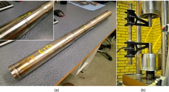
The margins of the fatigue design curve for austenitic stainless steel in ASME III [1] were subject to investigation in [4], where water pressurized welded stainless steel piping components were subjected to variable amplitude (VA) primarily reversed bending deformation, i.e. component testing or fatigue experiments under realistic conditions. The welded piping component and experimental set-up are illustrated in Figure 1. The nominal wall thickness in the central part of the test specimen, i.e. in the region including the circumferential butt weld, was 3 mm. The welding joint was in as-welded condition, i.e. the weld capping was not removed and induced a local stress concentration. Fatigue failure was defined by leakage, i.e. when the internal pressure of 70 bar could no longer be sustained. The experimental set-up was based on a construction using custom-built fixtures, which introduced a predominant bending stress and a small membrane stress. The work performed in [4] had particular focus on HCF and VA loading. The fatigue experiments included however both constant amplitude (CA) fatigue tests and experiments with VA loading using different load spectra, amongst which a synthetic Gaussian spectrum, designated with VAG. Additional information about the used test specimens, experimental set-up, testing procedure, load description and/or obtained results from the performed fatigue tests is available in [4, 5, 6, 7].

(a) (b)

Figure 1. (a) Welded piping component with close-up view of the circumferential butt weld in as-welded condition. (b) Actual mounted test specimen in servo-hydraulic testing machine with custom-built fixtures.

(12)

The performed work in [4] consisted of the determination of a component specific design curve derived from recorded nominal strain amplitudes. Comparison with the fatigue design curve in ASME III [1] allowed a better understanding of the margins in the ASME design curves and quantify the degree of conservatism. In the case of welded piping components, the presence of the welding joint induced a stress concentration. Hence the need to use a weld fatigue reduction factor to allow for the ASME fatigue design curve to be used in conjunction with nominal strain amplitudes. The work in [4] considered both a FSRF of 3.24 based on stress indices defined in NB-3600 of ASME III [1] and a FSRF approximated by a stress concentration factor of 1.4 computed by a finite element (FE) analysis. The findings in [4] highlighted extensive conservatism, but the extent of the margins in ASME was shown to largely depend on the weld fatigue reduction factor used.

2.3 Objectives

The current investigation is a continuation of the work performed in [4] and consists of fatigue tests on pressurized non-welded austenitic stainless steel piping components, with realistic VA loading and with particular focus on HCF. The empirical approach with a synthetic spectrum load developed in [4] will be applied. Through comparison with the results for the welded piping component in [4], a weld FSRF will be determined. The study will thus provide a revised and verified value for the weld fatigue reduction factor in [4]. The resulting margins in the fatigue design curve for austenitic stainless steel in ASME III [1] will be assessed by revising the findings from [4].

The work aims at

 increasing understanding of the effect of a welding joint on fatigue life for piping components by improving the knowledge about the difference in fatigue strength between non-welded and welded pipes.

 facilitating future discussions about margins and conservatism in ASME III [1].

 improving the knowledge on transferability for a non-welded piping component subjected to variable amplitude loading by comparing with smooth specimen data obtained with constant amplitude fatigue testing, see [2].  further increasing insight in how to efficiently handle and mitigate potential

fatigue risks in austenitic stainless steel components, i.e. increase fundamental understanding for fatigue in piping components.

(13)

The performed work in [4] consisted of the determination of a component specific design curve derived from recorded nominal strain amplitudes. Comparison with the fatigue design curve in ASME III [1] allowed a better understanding of the margins in the ASME design curves and quantify the degree of conservatism. In the case of welded piping components, the presence of the welding joint induced a stress concentration. Hence the need to use a weld fatigue reduction factor to allow for the ASME fatigue design curve to be used in conjunction with nominal strain amplitudes. The work in [4] considered both a FSRF of 3.24 based on stress indices defined in NB-3600 of ASME III [1] and a FSRF approximated by a stress concentration factor of 1.4 computed by a finite element (FE) analysis. The findings in [4] highlighted extensive conservatism, but the extent of the margins in ASME was shown to largely depend on the weld fatigue reduction factor used.

2.3 Objectives

The current investigation is a continuation of the work performed in [4] and consists of fatigue tests on pressurized non-welded austenitic stainless steel piping components, with realistic VA loading and with particular focus on HCF. The empirical approach with a synthetic spectrum load developed in [4] will be applied. Through comparison with the results for the welded piping component in [4], a weld FSRF will be determined. The study will thus provide a revised and verified value for the weld fatigue reduction factor in [4]. The resulting margins in the fatigue design curve for austenitic stainless steel in ASME III [1] will be assessed by revising the findings from [4].

The work aims at

 increasing understanding of the effect of a welding joint on fatigue life for piping components by improving the knowledge about the difference in fatigue strength between non-welded and welded pipes.

 facilitating future discussions about margins and conservatism in ASME III [1].

 improving the knowledge on transferability for a non-welded piping component subjected to variable amplitude loading by comparing with smooth specimen data obtained with constant amplitude fatigue testing, see [2].  further increasing insight in how to efficiently handle and mitigate potential

fatigue risks in austenitic stainless steel components, i.e. increase fundamental understanding for fatigue in piping components.

3 Experimental study

The results in the current investigation were obtained with a limited number of test specimens and realistic testing conditions.

3.1 Test specimens

A total of 19 test specimens were manufactured from straight, seamless TP 304 L stainless steel hot finished pipes. All specimens were manufactured from the same batch: lot 50260. Table 1 contains the chemical composition and Table 2 presents the tensile properties at room temperature of the material. The material was thus similar to the one used in [4], but the manufacturing process of the pipes did differ. The current pipes were hot worked (extruded), whereas the pipes in [4] were cold worked (rolling). The effect of this difference in manufacturing process on the fatigue material behavior of the test specimens was considered to be small.

Table 1. Chemical composition as percentage by weight [weight%] for lot 50260.

C Si Mn P S Cr Ni Mo Co Cu N

0.016 0.38 1.21 0.029 0.008 18.20 10.13 0.34 0.11 0.32 0.051 Table 2. Average tensile properties at room temperature for lot 50260.

Yield strength Rp0.2

[MPa] Tensile strength R[MPa] m Elongation [%] Young’s modulus E [GPa] (*) Poisson’s ratio [-]

240 600 60 200 0.3

(*) Sandvik 3R12

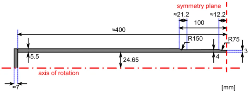
The original pipe geometry was identical to the one used in [4]: the pipe nominal outer diameter was 60.33 mm with a nominal wall thickness equal to 5.54 mm. The pipes were partially machined to introduce shoulders by reducing the outer diameter until a remaining wall thickness of approximately 4 mm. This first diameter reduction was introduced to reduce the risk for failure due to contact fatigue (fretting) under the fixtures. In order to further reduce the volume of material subjected to significant fatigue loads and localize fatigue failure, an additional diameter reduction was introduced in the center of the specimen. More specifically a circumferential notch with a fairly large notch radius of 75 mm was machined resulting in a nominal wall thickness of 3 mm in the symmetry plane of the test specimen. Figure 2 presents the geometry of the notched test specimens in more detail.

The internal surface roughness of the test specimens was somewhat greater in the current study than for the welded piping components used in [4]. However failure is expected to occur in the notch, i.e. on the external machined surface presenting a finer surface roughness. The increased surface roughness on the inside of the specimens is thus not expected to affect the fatigue behavior.

After machining of the test specimens, see Figure 3, the pipes were fitted with approximately 7 mm thick butt welded lids to allow pressurizing during the experiments. The lids were equipped with a fitting to allow control of the internal pressure.

(14)

Figure 2. Schematic of the geometry of the piping component.

Figure 3. Different test specimens after machining and prior to welding the lids at the extremities. [mm] ≈400 R150 R75 3 4 5.5 100 ≈7 24.65 ≈12.2 ≈21.2 symmetry plane axis of rotation

(15)

Figure 2. Schematic of the geometry of the piping component.

Figure 3. Different test specimens after machining and prior to welding the lids at the extremities. [mm] ≈400 R150 R75 3 4 5.5 100 ≈7 24.65 ≈12.2 ≈21.2 symmetry plane axis of rotation

3.2 Experimental set-up

3.2.1 Equipment and instrumentation

The experimental set-up consisted of the same custom-build construction as used in [4] allowing for reversed bending loading with displacement control in a standard single axis servo-hydraulic testing machine, see Figure 4. The distance between the grips was approximately 205 mm. Nominal (elastic) strains are linearly related to applied displacement, which supports the use of displacement control in the performed fatigue experiments [4]. Conventional strain gages were mounted on the test specimen in the axial direction at positions A and B, see Figure 4(b). The gage length was relatively short, 2 mm, allowing to get more accurate estimates of local peak values. Fatigue crack initiation was reported to occur in the vicinity of these locations for the experiments with welded piping components in [4]. These two positions are situated in the symmetry plane of the specimen, i.e. in the notch, and in the bending plane, i.e. the plane with the largest bending stresses. Position A is situated closest to the testing machine, where bending and membrane stresses act in phase, inducing maximum strain amplitudes. At position B the maximum bending stresses are in opposite phase from the membrane stresses resulting in somewhat lower maximum strain amplitudes [6]. The local axial strains in the notch were thus recorded during testing, as opposed to the nominal strain measure recorded in [4]. During the pre-testing phase of the experimental series some tests were however performed where also nominal axial strains were recorded similarly as in [4], i.e. approximately 50 mm from the notch.

(a) (b)

Figure 4. (a) Schematic of experimental set-up for alternating bending fatigue testing. (b) Schematic close-up view of the machined part of the specimen with the circumferential notch and strain gage positions A and B. non-welded piping component 300 load cell 70 bar circumferential notch prescribed displacement [mm] fixtures symmetry plane symmetry plane A circumferential notch B

(16)

3.2.2 Testing procedure

The fatigue experiments were displacement controlled with load ratio approximately equal to minus unity. Displacement control allows for realistic and relevant load definition. During the course of the fatigue experiments the resulting force in the load cell and the local axial strain measures at A and B for the test specimen were recorded with a sampling frequency of 200 Hz. The tests were performed in air at room temperature (RT), avoiding environmental effects on the fatigue behavior of the piping component, which was out of the scope of the current investigation. The piping components were furthermore water pressurized allowing for a realistic failure criterion based on leakage. The experiments were stopped when leakage was detected by the pressure actuator displacement increase to a pre-set level. Alternatively fatigue experiments were stopped when a run-out limit of 11000 load blocks (corresponding to approximately 5 million cycles) was reached or exceeded.

(17)

3.2.2 Testing procedure

The fatigue experiments were displacement controlled with load ratio approximately equal to minus unity. Displacement control allows for realistic and relevant load definition. During the course of the fatigue experiments the resulting force in the load cell and the local axial strain measures at A and B for the test specimen were recorded with a sampling frequency of 200 Hz. The tests were performed in air at room temperature (RT), avoiding environmental effects on the fatigue behavior of the piping component, which was out of the scope of the current investigation. The piping components were furthermore water pressurized allowing for a realistic failure criterion based on leakage. The experiments were stopped when leakage was detected by the pressure actuator displacement increase to a pre-set level. Alternatively fatigue experiments were stopped when a run-out limit of 11000 load blocks (corresponding to approximately 5 million cycles) was reached or exceeded.

3.3 Load description

The 19 piping components included in the experimental test series were mainly subjected to a synthetic Gaussian variable amplitude loading, which was scaled to 10 different severities, see Table 3. The bending deformation together with the internal pressure introduced a relevant multi-axial load state, as for the experiments in [4]. The constant internal pressure was 70 bar and yielded a tensile mean strain in the axial direction. The nominal axial strain contribution of the internal pressure was estimated to approximately ε0 = 0.0040 %, based on linear elastic material behavior.

This mean strain was considered small compared to the applied maximum strain amplitudes. Although increased test frequencies are convenient to reduce the total testing time, the testing frequency in the accelerated fatigue experiments was limited to avoid too large strain rates. No strain rate effects on the fatigue behavior were expected during the fatigue experiments at RT [2]. In the current investigations strain rates did usually not exceed 10%/s, except for cycles with large amplitudes in experiments with displacement amplitudes larger or equal to 4 mm.

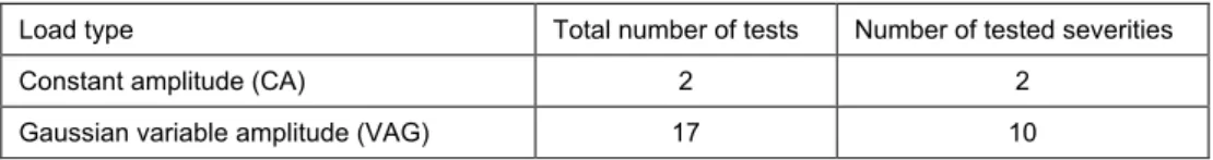
Table 3. Summary of different load types considered in the fatigue experiments.

Load type Total number of tests Number of tested severities

Constant amplitude (CA) 2 2

Gaussian variable amplitude (VAG) 17 10

3.3.1 Constant amplitude (CA)

The two constant amplitude experiments were performed with sinusoidal prescribed displacement signals. The severity of the prescribed displacement was determined by its amplitude: 1.95 or 3.1 mm. The corresponding local strain amplitudes in A were 0.17 and 0.23%, respectively.

3.3.2 Gaussian variable amplitude (VAG)

A Gaussian spectrum similar as the one used in [4] with 453 cycles per load block was used. A load block lasted 43.2 s and consecutive load blocks were separated by a brief transition or hold time. The hold time was in the range 0.5 - 1 s. A normalized load block is illustrated in Figure 5. The normalized axial strain signal was obtained by subtracting mean strain and dividing by the maximum strain amplitude. Ten severity levels were examined by scaling up the magnitude of the prescribed displacement. The recorded local maximum strain amplitude in A were in the range 0.2 – 0.4%, hence always exceeding the yield strain of 0.12%.

(18)

4 Theory and methods

4.1 Fatigue life models

Different models exist to predict the number of cycles to component failure as function of a load parameter, such as stress or strain amplitude. In the current experimental investigation the selected fatigue governing parameter was the measured strain amplitude, which allowed direct comparison with ASME predictions and further study of the ASME margins in the continuation of the work performed in [4].

The experimental results from the performed alternating fatigue bending tests on piping components were investigated with two different models with a scalar strain amplitude load parameter. The original models were generalized to be applicable with variable amplitude loading. A norm or equivalent strain amplitude was therefore introduced based on Palmgren-Miner’s linear damage rule [8, 9]. This hypothesis is in accordance with the ASME procedure. The methodology of this procedure is further detailed in [10] and is identical to the one applied in the previous work [4].

4.1.1 Basquin model

Basquin’s equation without a fatigue limit is a classic approach to model high cycle, low strain amplitude fatigue. A linear relation in logarithmic form is assumed, between the strain amplitude and the total number of load cycles, N [11]. In the current investigation with variable amplitude loading an equivalent strain amplitude ||εa||β is used,

𝑁𝑁 = 𝛼𝛼 ( ‖𝜀𝜀𝑎𝑎‖𝛽𝛽 )−𝛽𝛽 (1)

The constants α and β are typically determined by fitting to experimental data. The equivalent strain amplitude gives the same accumulated damage as the full spectrum and is defined as the β-norm of the strain amplitudes εa,i included in a load sequence

consisting of m strain cycles,

‖𝜀𝜀𝑎𝑎‖𝛽𝛽 = ( _{𝑚𝑚 ∑ 𝜀𝜀}1 𝑎𝑎,𝑖𝑖𝛽𝛽 𝑚𝑚 𝑖𝑖 ) 1/𝛽𝛽 (2)

(19)

4 Theory and methods

4.1 Fatigue life models

Different models exist to predict the number of cycles to component failure as function of a load parameter, such as stress or strain amplitude. In the current experimental investigation the selected fatigue governing parameter was the measured strain amplitude, which allowed direct comparison with ASME predictions and further study of the ASME margins in the continuation of the work performed in [4].

The experimental results from the performed alternating fatigue bending tests on piping components were investigated with two different models with a scalar strain amplitude load parameter. The original models were generalized to be applicable with variable amplitude loading. A norm or equivalent strain amplitude was therefore introduced based on Palmgren-Miner’s linear damage rule [8, 9]. This hypothesis is in accordance with the ASME procedure. The methodology of this procedure is further detailed in [10] and is identical to the one applied in the previous work [4].

4.1.1 Basquin model

Basquin’s equation without a fatigue limit is a classic approach to model high cycle, low strain amplitude fatigue. A linear relation in logarithmic form is assumed, between the strain amplitude and the total number of load cycles, N [11]. In the current investigation with variable amplitude loading an equivalent strain amplitude ||εa||β is used,

𝑁𝑁 = 𝛼𝛼 ( ‖𝜀𝜀𝑎𝑎‖𝛽𝛽 )−𝛽𝛽 (1)

The constants α and β are typically determined by fitting to experimental data. The equivalent strain amplitude gives the same accumulated damage as the full spectrum and is defined as the β-norm of the strain amplitudes εa,i included in a load sequence

consisting of m strain cycles,

‖𝜀𝜀𝑎𝑎‖𝛽𝛽 = ( _{𝑚𝑚 ∑ 𝜀𝜀}1 𝑎𝑎,𝑖𝑖𝛽𝛽 𝑚𝑚 𝑖𝑖 ) 1/𝛽𝛽 (2)

4.1.2 Langer model

The Langer model [12] uses a modified expression of the Basquin relation in Equation (1) including a cut-off limit introducing a characteristic curved shape for long lives. The design curves in the ASME standard [1] are based on fittings presented in [2] using the Langer model. The Langer equation is expressed in terms of constants A and B, analogues to α and β in Equation (1), and an additional constant

C introducing an asymptote in the model. For variable amplitude loading the

equivalent strain amplitude ||εa||BC is introduced,

𝑁𝑁 = 𝐴𝐴 ( ‖𝜀𝜀𝑎𝑎‖𝐵𝐵𝐵𝐵 − 𝐶𝐶 )−𝐵𝐵 (3)

The equivalent BC-norm of the strain amplitude gives the same accumulated damage as the full spectrum and is expressed, by analogy with Equation (2), in terms of constants B and C. ‖𝜀𝜀𝑎𝑎‖𝐵𝐵𝐵𝐵 = ( 1_{𝑛𝑛 ∑(𝜀𝜀}𝑎𝑎,𝑖𝑖− 𝐶𝐶)𝐵𝐵 𝑛𝑛 𝑖𝑖 ) 1/𝐵𝐵 + 𝐶𝐶 (4)

The sum only includes the n cycles for which the strain amplitudes exceed the threshold level C. Note that for C = 0, the Basquin relation from Equation (1) is recovered, i.e. all strain cycles of the considered load sequence contribute to fatigue damage accumulation.

4.1.3 Maximum-likelihood methodology

The maximum-likelihood methodology is a general method for fitting model parameters to empirical models. It is a probabilistic approach that as inputs needs,

i. a model formulation with parameters to be fit, ii. a number of empirical observations of a property,

iii. an assumption of a random distribution type for the observed property. In case of the two considered fatigue models the observed property is fatigue life and the two model formulations, Basquin and Langer have two and three fitting parameters, respectively. For each model, it is assumed that the logarithm of life follows a normal distribution with the expected value according to the model and an unknown standard deviation. The procedure used in the current investigation for determination of the model parameters is identical to the one applied in [4]. More details on the methodology are found in [10].

(20)

4.2 Transferability

The ANL mean curve from [2] was derived from fatigue tests on small, smooth test specimens. The current study performed however fatigue tests on a realistic smooth component. The expected difference in fatigue strength will illustrate the fundamental issue of transferability, i.e. the transfer from smooth test specimen results to predictions for real components. The former typically having a larger fatigue strength. In applications the fatigue strength of welded piping components is often limiting, as the welding joint introduces a stress concentration. The presence of a weld will result in a fatigue strength reduction of the component. The extent of this reduction can be quantified knowing the SN curve of the smooth component without a weld. The obtained SN curves from the current investigation correspond to those for the smooth piping component. Through comparison with the results for the welded piping component in [4], the amount of fatigue strength reduction can be determined.

4.2.1 FSRF estimation

The FSRF or the fatigue strength reduction factor is related to the fatigue strength measured as strain amplitude. The strain amplitude for the welded component should thus be multiplied with the FSRF to predict life using any of the plain piping fatigue models, Basquin or Langer.

By assuming that a constant FSRF fully describes the difference between plain and welded experimental results, Kf can be estimated from the recorded data. The

numerical procedure is based on a multiplication of the nominal weld strain amplitudes included in the applied Gaussian and piping spectra from [4]. The optimal factor being an estimate of Kf is then determined by the maximum-likelihood

procedure applied to both sets of experimental results, i.e. plain and welded. The considered fatigue model is thus fitted simultaneously to the valid VA data from the current study for non-welded specimens and scaled VA data from [4] for the welded pipes.

For the Basquin case, the model used in the likelihood estimation reads,

ln𝑁𝑁 = ln𝛼𝛼 − 𝛽𝛽 ln(‖𝑘𝑘 𝜀𝜀𝑎𝑎‖𝛽𝛽 ) = ln𝛼𝛼 − 𝛽𝛽 ln(𝑘𝑘‖𝜀𝜀𝑎𝑎‖𝛽𝛽 ) (5) Similarly, for the Langer case the model is given by,

ln𝑁𝑁 = ln𝐴𝐴 − 𝐵𝐵 ln( ‖𝑘𝑘 𝜀𝜀𝑎𝑎‖𝐵𝐵𝐵𝐵− 𝐶𝐶 ) (6) In these model formulations the scaling factor k = 1 for plain specimens and a positive constant for the welded piping components.

The possibility of a FSRF varying with amplitude was also considered. In the case of the Basquin model, such a variation would result in different slopes for welded and non-welded specimens when their parameters are estimated independently. The difference in slopes was a posteriori found not significant, which motivates the simple constant FSRF model used, see experimental results.

(21)

4.2 Transferability

The ANL mean curve from [2] was derived from fatigue tests on small, smooth test specimens. The current study performed however fatigue tests on a realistic smooth component. The expected difference in fatigue strength will illustrate the fundamental issue of transferability, i.e. the transfer from smooth test specimen results to predictions for real components. The former typically having a larger fatigue strength. In applications the fatigue strength of welded piping components is often limiting, as the welding joint introduces a stress concentration. The presence of a weld will result in a fatigue strength reduction of the component. The extent of this reduction can be quantified knowing the SN curve of the smooth component without a weld. The obtained SN curves from the current investigation correspond to those for the smooth piping component. Through comparison with the results for the welded piping component in [4], the amount of fatigue strength reduction can be determined.

4.2.1 FSRF estimation

The FSRF or the fatigue strength reduction factor is related to the fatigue strength measured as strain amplitude. The strain amplitude for the welded component should thus be multiplied with the FSRF to predict life using any of the plain piping fatigue models, Basquin or Langer.

By assuming that a constant FSRF fully describes the difference between plain and welded experimental results, Kf can be estimated from the recorded data. The

numerical procedure is based on a multiplication of the nominal weld strain amplitudes included in the applied Gaussian and piping spectra from [4]. The optimal factor being an estimate of Kf is then determined by the maximum-likelihood

procedure applied to both sets of experimental results, i.e. plain and welded. The considered fatigue model is thus fitted simultaneously to the valid VA data from the current study for non-welded specimens and scaled VA data from [4] for the welded pipes.

For the Basquin case, the model used in the likelihood estimation reads,

ln𝑁𝑁 = ln𝛼𝛼 − 𝛽𝛽 ln(‖𝑘𝑘 𝜀𝜀𝑎𝑎‖𝛽𝛽 ) = ln𝛼𝛼 − 𝛽𝛽 ln(𝑘𝑘‖𝜀𝜀𝑎𝑎‖𝛽𝛽 ) (5) Similarly, for the Langer case the model is given by,

ln𝑁𝑁 = ln𝐴𝐴 − 𝐵𝐵 ln( ‖𝑘𝑘 𝜀𝜀𝑎𝑎‖𝐵𝐵𝐵𝐵 − 𝐶𝐶 ) (6) In these model formulations the scaling factor k = 1 for plain specimens and a positive constant for the welded piping components.

The possibility of a FSRF varying with amplitude was also considered. In the case of the Basquin model, such a variation would result in different slopes for welded and non-welded specimens when their parameters are estimated independently. The difference in slopes was a posteriori found not significant, which motivates the simple constant FSRF model used, see experimental results.

4.2.2 Determination of ASME margins

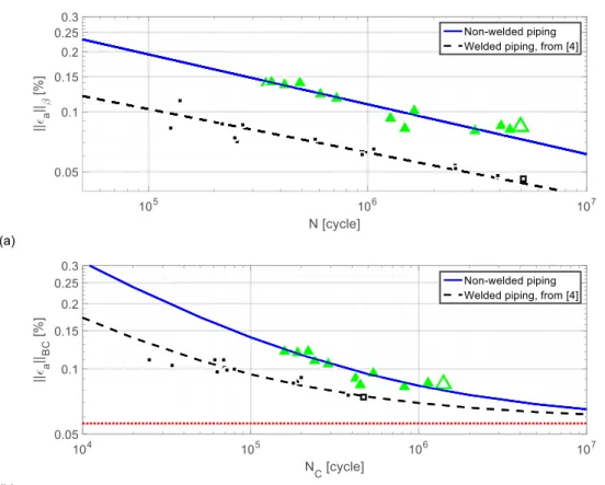
The margins of the ASME design curve are determined or quantified through comparison with component specific design curves derived with the empirical approach detailed in [4]. The parameter fitting with the maximum likelihood methodology results in an estimate of the standard deviation of logarithmic life. This estimate allows an approximate determination of the lower 90% prediction limit, which corresponds to a design curve for 95% survival probability. This design curve is component specific and can be compared to the corresponding design curve prescribed by ASME.

In the case of the current study the component specific design curve is derived with local strain amplitude measures, and can therefore be directly compared to the ASME design curve, which is intended for use in conjunction with local strain measures. In the case of the previous work with welded piping components [4], the recorded strain was the nominal strain. Hence the component specific design curve derived for the welded piping component is to be compared with a reduced ASME design curve, in order to get an estimate of its margins. The reduction of the ASME design curve was in [4] performed with different numerical estimates of the FSRF yielding relative uncertainty about the extent of the margins. In the current study however, the reduction is performed with an experimental estimate of the FSRF.

(22)

5 Results

5.1 Preliminary investigation

5.1.1 Notch effect

The CA test of pipe 02 was apart from strain recordings for the local strains in the notch also equipped for nominal strain readings with an additional strain gage positioned about 50 mm from the notch, i.e. similar as in [4]. The start of the experiment included a short sequence with low strain amplitudes ensuring fully elastic material behavior even in the notch. Comparison between the local strain in the notch and the nominal strain resulted in an estimated (elastic) notch factor Kt|t = 4 mm = 1.6. This notch factor designates the elastic strain concentration in the notch to

the nominal strain recorded for a wall thickness equal to 4 mm. The welded piping component in [4] did however have a wall thickness of 3 mm. Through conservation of internal bending moment, the ratio of elastic nominal strains can be approximated by the inverse of the ratio of the nominal wall thicknesses. Hence, Kt|t = 3 mm ≈ 0.75

Kt|t = 4 mm, which yields an updated (elastic) notch factor Kt|t = 3 mm = 1.2. The strain in

the notch of the investigated piping component is thus about 20% larger than the expected nominal strain for the corresponding un-notched piping component with wall thickness 3 mm.

The fatigue strength reduction factor Kf is defined as the ratio of the fatigue strength

for the un-notched specimen and the fatigue strength for the notched specimen. The fatigue strengths considered are taken for a given number of cycles. Different numerical or analytical methods to estimate the fatigue strength reduction factor Kf

accounting for the presence of the notch exist [13, 14]. A classic approach is to relate the FSRF to the notch or elastic stress/strain concentration factor Kt by means of the

notch sensitivity factor q varying between 0 and 1,

𝐾𝐾f = 1 + 𝑞𝑞( 𝐾𝐾t− 1 ) (7)

For q = 0, the material is considered to be notch insensitive and Kf = 1, i.e. that the

presence of a notch does not affect the fatigue strength, as plastic deformation in the notch effectively reduces the stress concentration. However for q = 1 or large notch sensitivity of the material, the FSRF is considered equal to the notch factor, i.e. Kf =

Kt. In this case no redistribution of stress through local plasticity is expected. For

common steels the notch sensitivity is expected to be close to unity given the large notch radius equal to 75 mm. However austenitic steels are known to present good notched fatigue strength, and thus a relatively low notch sensitivity [15]. Handbook recommendations [16] consider for annealed austenitic stainless steel that q is in the range 0.2 – 0.4 and increases with Kt. For the current application the notch factor is

fairly low, hence a notch sensitivity of 0.3 can be considered as a conservative estimate. Consequently the FSRF for the notched smooth piping component compared to a smooth un-notched piping component with wall thickness 3 mm is equal to Kf = 1+ 0.3 (1.2-1) =1.06, which is very close to unity.

(23)

5 Results

5.1 Preliminary investigation

5.1.1 Notch effect

The CA test of pipe 02 was apart from strain recordings for the local strains in the notch also equipped for nominal strain readings with an additional strain gage positioned about 50 mm from the notch, i.e. similar as in [4]. The start of the experiment included a short sequence with low strain amplitudes ensuring fully elastic material behavior even in the notch. Comparison between the local strain in the notch and the nominal strain resulted in an estimated (elastic) notch factor Kt|t = 4 mm = 1.6. This notch factor designates the elastic strain concentration in the notch to

the nominal strain recorded for a wall thickness equal to 4 mm. The welded piping component in [4] did however have a wall thickness of 3 mm. Through conservation of internal bending moment, the ratio of elastic nominal strains can be approximated by the inverse of the ratio of the nominal wall thicknesses. Hence, Kt|t = 3 mm ≈ 0.75

Kt|t = 4 mm, which yields an updated (elastic) notch factor Kt|t = 3 mm = 1.2. The strain in

the notch of the investigated piping component is thus about 20% larger than the expected nominal strain for the corresponding un-notched piping component with wall thickness 3 mm.

The fatigue strength reduction factor Kf is defined as the ratio of the fatigue strength

for the un-notched specimen and the fatigue strength for the notched specimen. The fatigue strengths considered are taken for a given number of cycles. Different numerical or analytical methods to estimate the fatigue strength reduction factor Kf

accounting for the presence of the notch exist [13, 14]. A classic approach is to relate the FSRF to the notch or elastic stress/strain concentration factor Kt by means of the

notch sensitivity factor q varying between 0 and 1,

𝐾𝐾f= 1 + 𝑞𝑞( 𝐾𝐾t− 1 ) (7)

For q = 0, the material is considered to be notch insensitive and Kf = 1, i.e. that the

presence of a notch does not affect the fatigue strength, as plastic deformation in the notch effectively reduces the stress concentration. However for q = 1 or large notch sensitivity of the material, the FSRF is considered equal to the notch factor, i.e. Kf =

Kt. In this case no redistribution of stress through local plasticity is expected. For

common steels the notch sensitivity is expected to be close to unity given the large notch radius equal to 75 mm. However austenitic steels are known to present good notched fatigue strength, and thus a relatively low notch sensitivity [15]. Handbook recommendations [16] consider for annealed austenitic stainless steel that q is in the range 0.2 – 0.4 and increases with Kt. For the current application the notch factor is

fairly low, hence a notch sensitivity of 0.3 can be considered as a conservative estimate. Consequently the FSRF for the notched smooth piping component compared to a smooth un-notched piping component with wall thickness 3 mm is equal to Kf = 1+ 0.3 (1.2-1) =1.06, which is very close to unity.

The notch was introduced to localize fatigue failure and reduce the volume of tested material. It will inevitably induce a reduction of the components fatigue strength compared to the un-notched specimen. For the current test series however the reduction is considered negligible. As a result, the smooth piping component with a large machined notch used in the current study has a fatigue strength similar to the un-notched smooth piping component with wall thickness 3 mm. This is an important result as knowledge about the reference fatigue strength curve for the un-notched smooth piping component is crucial in the experimental determination of the FSRF for the welded piping component in [4].

5.1.2 Inelastic material behavior

Inelastic deformations at relatively low loads are reported for austenitic stainless steel in [17]. During fatigue testing of the welded piping components in [4], the nominal strain recordings also indicated non-linear material behavior. In the current investigation similar non-linear material behavior was therefore expected and indeed observed. The observation of non-linear material behavior was even more pronounced as, contrary to the previous study, the local strain in the notch was recorded. Load spectra did indeed always include a certain amount of load cycles inducing strain amplitudes exceeding the material’s yield strain. As a result, plastic deformations were rapidly induced in the vicinity of the locations A and B in the notch.

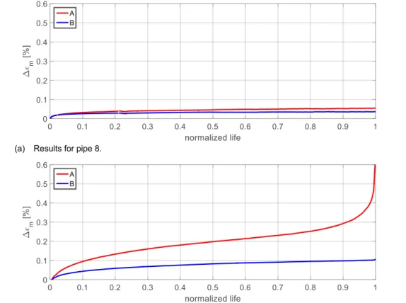
(a) Results for pipe 8.

(b) Results for pipe 14.

Figure 6. Illustration of the recorded increase in local axial mean strain (Δεm) in both A and B locations

(24)

The internal pressure is a primary load and introduces a tensile axial mean strain. It was however observed that the axial mean strain increased during fatigue testing, especially in the case of significant cyclic loading. A cyclic secondary load, introduced through prescribed displacement, consists of reversed bending and membrane loads. The austenitic stainless steel piping component subjected to this load combination exhibited ratchetting behavior, i.e. progressive accumulation of inelastic strain. The accumulation of inelastic strain did have little effect on the recorded strain amplitude used in the fatigue assessment, but affected considerably the mean axial strain. Figure 6 illustrates, for a selection of two tests, the increase in axial mean strain recorded in the notch as function of the normalized testing time or fatigue life. The increase in location A always exceeded the one recorded in B. The difference in ratchetting behavior between A and B is explained by the difference in cyclic deformation at these locations. For relatively low cyclic loading, see Figure 6 (a), the progressive accumulation of inelastic axial strain occurs primarily during the early stages of the test. After this initial period the accumulation or increase in axial mean strain is relatively small or negligible. However for increased cyclic loading, see Figure 6 (b), significant accumulation of inelastic axial strain continued during the entire experiment.

(25)

The internal pressure is a primary load and introduces a tensile axial mean strain. It was however observed that the axial mean strain increased during fatigue testing, especially in the case of significant cyclic loading. A cyclic secondary load, introduced through prescribed displacement, consists of reversed bending and membrane loads. The austenitic stainless steel piping component subjected to this load combination exhibited ratchetting behavior, i.e. progressive accumulation of inelastic strain. The accumulation of inelastic strain did have little effect on the recorded strain amplitude used in the fatigue assessment, but affected considerably the mean axial strain. Figure 6 illustrates, for a selection of two tests, the increase in axial mean strain recorded in the notch as function of the normalized testing time or fatigue life. The increase in location A always exceeded the one recorded in B. The difference in ratchetting behavior between A and B is explained by the difference in cyclic deformation at these locations. For relatively low cyclic loading, see Figure 6 (a), the progressive accumulation of inelastic axial strain occurs primarily during the early stages of the test. After this initial period the accumulation or increase in axial mean strain is relatively small or negligible. However for increased cyclic loading, see Figure 6 (b), significant accumulation of inelastic axial strain continued during the entire experiment.

5.2 Experimental fatigue results

A total of 19 fatigue experiments were performed during the current study. Only 13 experiments were however considered valid for performing the projected investigation. The results of these experiments are reported in Table 4 and Figure 7. The piping components were water pressurized which allowed for the failure criterion based on leakage. The presence of water drops in the circumferential notch was an illustration of ongoing leakage, see Figure 8, and indicating the presence of a penetrating fatigue crack. Only one experiment (pipe 8) was terminated prior to leakage detection, as the run-out limit of 11000 load blocks was reached. The total number of strain cycles to which each tested piping component was subjected is denoted N, including thus also strain cycles with small strain amplitudes contained in the VAG load spectra. The different equivalent strain measures were computed once the model parameters were estimated, see Section 5.2.2, from the local axial strain recordings in location A. All valid fatigue tests presented leakage in the vicinity of A, where the strain amplitudes were in average about 15% higher than those recorded in B. Locations A and B are defined in Figure 4.

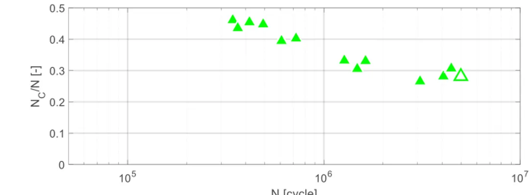
The total number of strain cycles actually causing fatigue damage according to the Langer model is given by NC. This quantity was computed by only considering the

strain cycles to failure with amplitudes exceeding the threshold C. The BC-norm strain and NC are directly related. NC < N for the data points which yields a shift

leftwards in Figure 7, when only the number of cycles actually causing fatigue damage would be considered instead of the total number of cycles to failure. Table 4. Experimental results from valid VAG fatigue tests. The β-norm was computed with β= 4.0 and the BC-norm with B = 2.07 and C= 0.056%. The strain measures are all based on the recorded local strain in location A. Pipe ID Severity (*) _N _{max ε} a ||εa||β ||εa||BC NC [cycles] [%] [%] [%] [cycles] 4 4 608832 0.35 0.123 0.109 240119 6 3.7 1270665 0.25 0.093 0.091 421851 (†)8 3 4983000 0.23 0.084 0.085 1400843 9 3.3 1630347 0.28 0.101 0.095 537982 10 3.05 4061145 0.23 0.085 0.086 1139689 11 4.3 343374 0.39 0.140 0.121 158269 12 4.3 363759 0.41 0.141 0.120 158599 13 3.05 4449819 0.21 0.082 0.084 1364373 14 4 719364 0.33 0.117 0.105 289784 15 4.5 490146 0.39 0.139 0.120 219483 16 3.4 1474968 0.21 0.082 0.084 450191 17 3.2 3093084 0.22 0.080 0.082 822439 19 4.5 416760 0.38 0.137 0.118 189513

(*)_{The severity corresponds approximately to the maximum prescribed displacement amplitude in mm.}

(26)

Figure 7. Experimental results with different strain measures for the 13 valid fatigue experiments on smooth piping components. The empty marker indicates a run-out and the numbers next to the black markers correspond to the pipe ID.

Figure 8. Axial strain gage mounted in the circumferential notch and water drops indicating leakage.

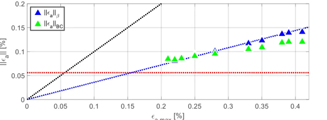
Figure 9. Relation between equivalent strain measures and maximum strain amplitude in the VAG spectrum. The β-norm was computed with β = 4.0 and the BC-norm with B = 2.07 and C= 0.056%.

11 12 19 15 4 14 6 16 9 17 10 13 8

(27)

Figure 7. Experimental results with different strain measures for the 13 valid fatigue experiments on smooth piping components. The empty marker indicates a run-out and the numbers next to the black markers correspond to the pipe ID.

Figure 8. Axial strain gage mounted in the circumferential notch and water drops indicating leakage.

Figure 9. Relation between equivalent strain measures and maximum strain amplitude in the VAG spectrum. The β-norm was computed with β = 4.0 and the BC-norm with B = 2.07 and C= 0.056%.

11 12 19 15 4 14 6 16 9 17 10 13 8

Contrary to the maximum strain amplitude, the equivalent strain measures account for the presence of lower strain amplitudes included in the load sequence. Hence the considerably lower values presented for the fatigue results with the VAG spectrum in Figure 7. Considering that even lower strain amplitudes will contribute to fatigue damage accumulation, the maximum strain amplitude will represent an over-estimation of the effective load. The equivalent strain measures are therefore more appropriate as fatigue parameters for VA loading. Figure 9 illustrates in more detail the relation between the equivalent strain measures and the local maximum strain amplitude. CA data points would be situated on the first bissectrice represented by the black dotted line. VA data points are however expected to be situated below the first bissectrice.

For a given spectrum, a proportional relation exists between the β-norm and the maximum strain amplitude of the considered spectrum. The constant of proportionality is, for a given spectrum, solely dependent on the value of β. For the current study considering the VAG spectrum with β = 4.0, the constant of proportionality is about 0.36, which is illustrated graphically by the blue dotted line in Figure 9. The β-norm in the current study is indeed about 36% of the maximum strain amplitude. More generally, for any spectrum the ratio of proportionality increases with β and tends to 1 for large values of β. For β tending to infinity, the infinity norm or maximum norm is indeed recovered, which then equals the maximum strain amplitude of the spectrum. In the case of the BC-norm, no proportional relation can be defined due to the effect of the cut-off limit C in the definition of the norm. The threshold level is represented in Figure 9 by the red dotted horizontal and acts as a lower limit of the BC-norm. It may be noted that the β- and

BC-norms in the current study yield fairly similar magnitudes of the equivalent local

strain measure.

5.2.1 Excluded experiments

A total of 6 experiments were excluded or considered as non-valid. The initial two CA tests (pipes 1 and 2) were part of a pre-testing phase. They were mainly intended to facilitate the initial set-up of the experimental procedure and get an initial estimate of the fatigue strength of the selected piping geometry. Pipes 1 and 2 were respectively subjected to approximately 94000 and more than 2 million cycles prior to failure. Pipe 1 did however present leakage in location B and pipe 2 failed under a clamp of the fixture, see Figure 10, presumably due to fretting fatigue. It motivated preemptive measures to improve the surface roughness under the clamps, which successfully prevented fretting fatigue in the VA tests.

Pipes 3, 5, 7 and 18, were subjected to a VAG spectrum load sequence with maximum strain amplitude of about 0.3, 0.3, 0.2 and 0.15%, respectively. The total number of applied cycles for these four experiments was approximately 1124000, 543000, 1161000 and more than 13 million cycles.

 Pipe 3 failed in location B due to increased friction in the experimental set-up, which was remediated for consecutive experiments.

 Pipe 5 failed consistently in A, but the data collection failed unfortunately at an early stage of the experiment and was therefore considered non-valid.  Pipe 7 presented also a consistent final failure in A, but was considered

(28)

test. The test was terminated prior to leakage or failure and thus considered a run-out.

As a result of the above irregularities, these four VA tests were thus not included in the projected analysis. The current test series did thus provide 13 valid data points for the analysis. It may be noted that the previous investigation for welded piping component in [4] also considered 13 data points from the VA piping and Gaussian spectra experiments. The number of valid data points was considered to be sufficient to avoid too large variance in the computed results.

Figure 10. Failure of pipe 2 below a clamp of the fixture due to fretting fatigue.

5.2.2 Parameter estimation

The model parameters for the smooth piping component were estimated using only the experimental data from the valid VAG load sequences reported in Table 4, i.e. 13 observations were used. The estimated parameters for both investigated fatigue life models are presented in Table 5. For the Basquin relation only two parameters were estimated, α and β, whereas the parameters in the Langer equation are A, B and

C. The estimated standard deviation of the random error in the logarithmic fatigue

life is denoted 𝜎𝜎𝜎. It is approximately equal to the coefficient of variation of the fatigue life. The corresponding results for the welded piping component are reported in Table 6, which is reproduced from [4].

Table 5. Estimated model parameters and standard deviation of the random error based on the VAG data for the non-welded piping component.

Model: Factor Slope Cut-off limit 𝜎𝜎𝜎

Basquin 𝛼𝛼𝜎 141 𝛽𝛽̂ 4.0 - 0.36

Langer 𝐴𝐴̂ 591 𝐵𝐵̂ 2.07 𝐶𝐶̂ 0.056 % 0.36

Table 6. Estimated model parameters and standard deviation of the random error for the welded piping component in [4].

(29)

test. The test was terminated prior to leakage or failure and thus considered a run-out.

As a result of the above irregularities, these four VA tests were thus not included in the projected analysis. The current test series did thus provide 13 valid data points for the analysis. It may be noted that the previous investigation for welded piping component in [4] also considered 13 data points from the VA piping and Gaussian spectra experiments. The number of valid data points was considered to be sufficient to avoid too large variance in the computed results.

Figure 10. Failure of pipe 2 below a clamp of the fixture due to fretting fatigue.

5.2.2 Parameter estimation

The model parameters for the smooth piping component were estimated using only the experimental data from the valid VAG load sequences reported in Table 4, i.e. 13 observations were used. The estimated parameters for both investigated fatigue life models are presented in Table 5. For the Basquin relation only two parameters were estimated, α and β, whereas the parameters in the Langer equation are A, B and

C. The estimated standard deviation of the random error in the logarithmic fatigue

life is denoted 𝜎𝜎𝜎. It is approximately equal to the coefficient of variation of the fatigue life. The corresponding results for the welded piping component are reported in Table 6, which is reproduced from [4].

Table 5. Estimated model parameters and standard deviation of the random error based on the VAG data for the non-welded piping component.

Basquin 𝛼𝛼𝜎 141 𝛽𝛽̂ 4.0 - 0.36

Langer 𝐴𝐴̂ 591 𝐵𝐵̂ 2.07 𝐶𝐶̂ 0.056 % 0.36

Table 6. Estimated model parameters and standard deviation of the random error for the welded piping component in [4].

(a)

(b)

Figure 11. Estimated mean fatigue curves using the (a) Basquin fatigue model, and (b) Langer fatigue model with the red dotted horizontal representing C for the non-welded piping.

Figure 11 illustrates the obtained fittings for the non-welded or plain piping component with both considered fatigue models, see the blue solid curves and green triangular data points. The red dotted horizontal in Figure 11 (b) represents the value of the cut-off limit C obtained for the smooth non-welded piping component. The fitted mean curves and data points for the welded piping component studied in [4] are added for comparison in Figure 11, see the black dashed curves and square data points. Note however that the equivalent strain amplitudes for the welded component were computed based on the values for β, B and C reported in Table 6 or [4]. Comparison of Table 5 with the parameter estimates obtained for the welded piping component in Table 6 shows similar results for β, B and C. The difference in Basquin slopes for the welded and non-welded components can indeed be considered to be small, as illustrated graphically in Figure 11 (a). The 95% confidence interval (CI) of the difference in slope is estimated to (-1.02, 2.16), hence the difference is insignificant. However considerable differences for the factors α and A are observed, when comparing Table 5 and Table 6. The estimates for the non-welded component are indeed considerably larger than those obtained for the welded component. These factors directly relate to the vertical shift of the respective fatigue models, see Figure 11. Increased estimates of the factors α and A compared to the results related to the welded piping component is consistent with increased fatigue resistance for the smooth non-welded specimen.

The coefficients of variation of the estimated fatigue life in Table 5 are equal or smaller than those for the welded piping component in Table 6. A somewhat larger variation in fatigue life for a welded component may be related to a larger variation

2017:25 Evaluation of weld fatigue reduction in austenitic stainless steel pipe components

Research

Evaluation of weld fatigue reduction

in austenitic stainless steel pipe

components

2017:25

2017:25

Evaluation of weld fatigue reduction

in austenitic stainless steel pipe

Evaluation of weld fatigue reduction

in austenitic stainless steel pipe

components

Summary

Contents

Contents

1 Nomenclature

2 Introduction

2.1 Background

2 Introduction

2.1 Background

2.2 Performed Piping Component Fatigue Tests

2.3 Objectives

2.3 Objectives

3 Experimental study

3.1 Test specimens

3.2 Experimental set-up

3.2.1 Equipment and instrumentation

3.2.2 Testing procedure

3.2.2 Testing procedure

3.3 Load description

3.3.1 Constant amplitude (CA)

3.3.2 Gaussian variable amplitude (VAG)

4 Theory and methods

4.1 Fatigue life models

4.1.1 Basquin model

4 Theory and methods

4.1 Fatigue life models

4.1.1 Basquin model

4.1.2 Langer model

4.1.3 Maximum-likelihood methodology

4.2 Transferability

4.2.1 FSRF estimation

4.2 Transferability

4.2.1 FSRF estimation

4.2.2 Determination of ASME margins

5 Results

5.1 Preliminary investigation

5.1.1 Notch effect

5 Results

5.1 Preliminary investigation

5.1.1 Notch effect

5.1.2 Inelastic material behavior

5.2 Experimental fatigue results

5.2.1 Excluded experiments

5.2.2 Parameter estimation

5.2.2 Parameter estimation