Development of deterioration
models for cold climate using
long-term pavement field data
Paper presented at the 8th International conference
on Asphalt Pavements in Seattle Washington,
USA, August 10 14, 1997
Nils-Gunnar Göransson, Sweden
W. Ronald Hudson, USA
Heikki Jämsä, Finland
Harri Spoo Finland
Lars-Göran Wågberg, Sweden
[N
G")
c»
H N hN
x
0 >. h 4.0 h 36 UI"'ai
Swedish National Road and
VTI särtryck
No. 277 ' 1997
Development of deterioration models for cold
climate using long-term pavement field data
Paper presented at the 8th International conference
on Asphalt Pavements in Seattle, Washington, USA,
August 10 14, 1997
Nils-Gunnar Göransson, Sweden
W. Ronald Hudson, USA
Heikki Jämsä, Finland
Harri Spoof, Finland
Lars-Göran Wågberg, Sweden
Swedish National Road and
'ii'anspart Research Institute
DEVELOPMENT OF DETERIORATION MODELS FOR
COLD CLIMATE USING LONG-TERM PAVEMENT
FIELD DATA
Heikki Jämsä
Senior Research Engineer
Head of Infrastructure and Environmental
Engineering
Technical Research Centre of Finland
(VTT)
P.O. Box 19031
02044 VTT
Finland
Lars Göran Wågberg
Senior Research Engineer
Swedish Road and Transport
Research Institute (VTI)
S 58 195 Linköping
Sweden
Harri Spoof
Research Engineer
Technical Research Centre of Finland
(VTT)
Nils-Gunnar Göransson
Research Engineer
Swedish Road and Transport
Research Institute (VTI)
W. Ronald Hudson
Dewitt C. Greer Centennial Professor in Civil Engineering
The University of Texas at Austin
Department of Civil Engineering
Austin, Texas 787 12 1076
Abstract The paper describes the results of the Long-Term Pavement Performance (LTPP) study carried out in Finland and Sweden on the GPS-l experiment (asphalt concrete on granular base). The main results include new pavement deterioration models which are based on a failure time approach using censored data on 64 test sections. A large number of independent variables were examined to identify factors which explain most of the pavement deterioration on wheel paths (traffic related distress) and on a whole pavement surface (traffic and climate related distress). The most important factors explaining deterioration included tensile strain at the bottom of the asphalt layer, or the surface curvature index calculated from FWD measurements and the freezing index. In addition to
USA
deterioration models, a new neural network approach to calculate tensile strains on the basis of measured deflection bowl and asphalt layer thickness is introduced.
Keywords: Deterioration, modeling, failure time, neural networks, pavement response, service life.
1. INTRODUCTION
In Finland and Sweden road construction is in uenced by the interaction of traffic loading and cold climate which set great demands on the functional and structural performance of pavements. The long-term field performance of pavements has not yet been fully understood due to the complexity of the deterioration
process. In some cases this has resulted in unpredictable failures of existing roads and in some cases roads have been over-designed, causing uneconomical pavement structures.
In order to investigate the field performance of existing pavements, Finland and Sweden together with Denmark and Norway are taking part in the Long-Term Pavement Performance (LTPP) study initiated by SHRP (Strategic Highway Research Program) /1/. The research project focuses on the GPS-1 experiment (asphalt concrete on granular base). This paper describes the results derived from the Finnish and Swedish LTPP test sections.
2. OBJECTIVES
The objective of this research is to develop structural deterioration models for use in pavement management systems and design equations for pavements in a wet freeze climate. In this study the structural deterioration relates to cracking of a pavement due to fatigue and uneven frost heave. Models are developed for newly constructed exible pavements with unbound base using long-term monitoring data from in-service pavements in Finland and Sweden.
Specific objectives of the study are as follows: o to determine the effects of explanatory variables
(pavement structure, subgrade, traffic, environment) on the structural deterioration of pavement,
o to assess the effect of pavement response on deterioration,
o to develop new deterioration models for asphalt concrete pavements.
3. SELECTION OF TEST SECTIONS The study includes in-service pavement test sections from Finland and Sweden selected for the Nordic SHRP LTPP project in 1990. In addition, the data base includes sections that are part of the Swedish national study initiated in 1985.
Pavements consist of a hot mix asphalt concrete surface layer placed over an untreated granular base. The test sections are in their first structural performance year. No significant rehabilitation, strengthening or overlay have been applied to the pavement since it was constructed. Two consecutive lifts of the same mixture are treated as one layer. Test sections with stage
construction (common practice in the Nordic countries) have been accepted in the data base if an additional surface layer was added within two years after opening the test section to traffic when there were no distresses on the original surface layer.
Original SHRP-LTPP test sections are 150 meters in length and one lane in width. Sections that are part of the Swedish national study are 100 meters in length. These have been converted by multiplication to correspond to a length of 150 meters. Sections were selected based on the following general criteria according the SHRP guidelines:
. surface courses or overlays containing recycled or reclaimed asphalt concrete pavement as a component were not accepted,
0 there are no intersections, ramps, stop signs or other features close to the section which in uence traffic movement over the test section, . sections locate at grade or within consistent cut or fill with the depth of cut or fill approximately constant throughout the section in order to avoid inconsistent subgrade support and drainage conditions,
' transitional areas (cut to fill, shallow ll to deep fill, etc.) were avoided,
. test sections with added or widened lanes or shoulders were not accepted.
The object of the study is to develop deterioration models which cover a wide variety of design practices, environments and traffic conditions. The selection process of candidate test sections was based on the experimental design principles. This approach was chosen to ensure in advance that it is possible to find a correlation between dependent and independent variables which explain pavement deterioration. In addition, experimental design allows selection of test sections in the most cost effective way regarding the number of sections and money available. A sampling design was developed that consisted of the following factors considered most relevant to pavement deterioration:
. environment, 0 traffic, 0 subgrade,
' asphalt concrete thickness, . bearing capacity (de ection).
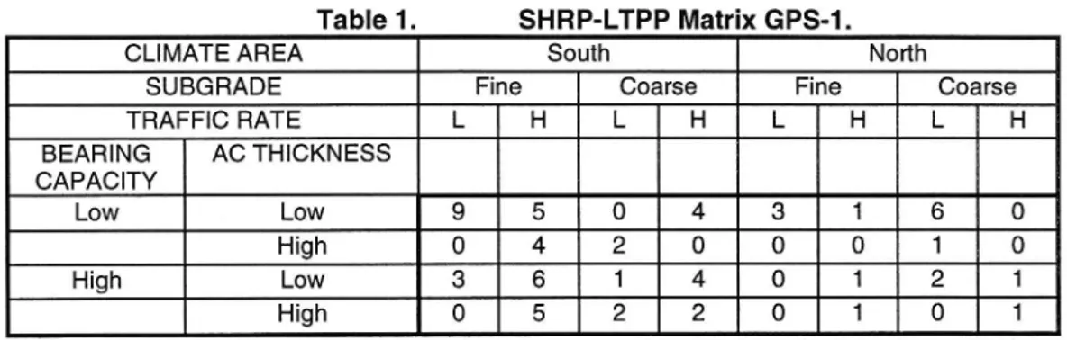
Table 1 shows the sampling frame and the distribution of GPS-1 test sections. Numbers in the frame indicate the number of test sections in each cell.
Table 1.
SHRP-LTPP Matrix GPS-1.
CLIMATE AREA South North
SUBGRADE Fine Coarse Fine Coarse TRAFFIC RATE L H L H L H L H BEARING AC THICKNESS CAPACITY Low Low 9 5 O 4 3 1 6 0 High O 4 2 0 O O 1 0 High Low 3 6 1 4 0 1 2 1 High O 5 2 2 O 1 O 1
Factor midpoints were used as selection criteria for each factor level. The following values were selected on the basis of experience and current construction practice:
Variable Factor midpoint . Climate area -15000 h°C 0 Subgrade Fine, coarse . Traffic rate 2500 vehicles/day O Bearing capacity 430 MPa
0 AC thickness 80 mm
The freezing index (climate area) takes different environmental conditions into account. The area ranges from the southern part of Sweden to the northern part of Finland. The traffic factor has two levels based on the traffic volume (average annual daily traffic). Two different subgrade types (fine and coarse) were considered. Factor midpoint for asphalt concrete (AC) thickness was selected as a value between one layer (usually 50 mm) and two layers (100 mm). The bearing capacity value is based on current structural design guidelines.
The total number of test sections in the data base is 64, of which 18 are from Finland and 46 from Sweden.
4. DATA COLLECTION AND DESCRIPTION In order to ensure the maximum utility and joint bene t of correlated LTPP studies, Finland and Sweden try to provide as far as possible data with the same type of equipment and the same procedures as outlined for LTPP by SHRP /2, 3/.
True pro les (transverse, longitudinal) of test sections have been measured using road surface monitoring vehicles available in each country. Information is processed to calculate the International Roughness Index (IRI) values for each test section. De ection measurements have been carried out with falling-weight de ectometers manufactured by Dynatest (Finland) and KUAB (Sweden). The surface condition is evaluated visually according to the Distress Identi cation Manual for the Long-Term Pavement Performance program on an annual basis.
One test pit was made for original SHRP-LTPP test sections in order to determine layer thickness, grain size distributions and density of each layer. Test pits were located at the end of a test section. Some data from the Swedish national study is based on nominal thickness information derived from design plans. Other data items collected include among other things pavement age, traf c volume and the number of equivalent single axle loads (measured or estimated). Measured data is stored in the Nordic data base located at the Technical Research Centre of Finland.
Frost is one of the important factors which must be taken into account in Nordic pavement design practice. The freezing index varies between -9000
h°C and -27000 hOC. For this reason typical
pavements consist of thin overlays combined with thick unbound layers. This is illustrated in gures 1 and 2 which show the distribution of layer thickness of test sections. AC thickness varies between 40 mm and 150 mm (average of 80 mm). The thickness of unbound layers ranges from 500 mm to 1600 mm (average 700 mm).
35 100 % ;, ~ 90 % 30 __ (å 80 % Q '
5 25 "
70 %
ä l Frequency _ 60 o/ 20 __ . O i?) + Cumulative % E är? -__ 50 % LL '.:o 15
-- 40 %
55 45; g 10 - åå 30 %%
ååå- %
20 %
%% 10 /o 0 * "ååå - 0 % 40 60 80 100 120 140 More THICKNESSFigure 1. Distribution of AC thickness (mm).
40 100 % 35 __ - 90 % cg 80 % g 30 -5 70 % LU __ if 25 » . Frequency 60 % CD + Cumulative % E 20 ~ 50 % LI. % 30 cy % 10 Z " 20 0/0
5 _
~ 10 %
0 - o % 500 700 900 1 100 1300 THICKNESS 1500 MoreFigure 2. Distribution of the thickness of unbound layers (mm).
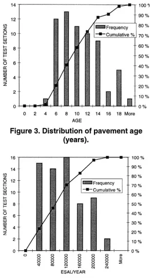
The age of test sections in 1995 varies between 4 and 24 years average being 10 years ( gure 3). Figure 4 illustrates the cumulative number of equivalent single axle loads (ESAL s, 10 tons) per year that test sections have. The average value is 95000 ESAL's/year. 14 100 % 12 __ 90 % 2 Frequency 80 % å 10 __ +Cumulative % 70 % g 8 __ " 60 °/o E " 50 % å 6 " 40 % % 4 __ "' 30 % z ~- 20 % 2 " - 10 % 0 _ 0 % 0 2 4 6 8 10 12 AGE 14 16 18 More
Figure 3. Distribution of pavement age
(years).
16 100 % 14 ... " 90 % % 12 80 % 5 Frequency __ 70 % Lu 10 _ +Cumulative % w 60 % 17> |ill J 8 _ " 50 °/o LI. O _ -- 40 % m 6 lä 30 % ä 4 3 20 % 2 _ - 10 % 0 ' O O 0 % O O O O O O O <1-N N EsAL/véÄRFigure 4. Distribution of the cumulative
number of equivalent single axle loads l year
(10 tons).
For analysis purposes a distress index was developed which takes into account the amount and severity level of each distress type. The distress index is computed first by multiplying the amount of each distress type occurring on a pavement surface by the weighing factor and by the corresponding severity level factor, respectively. Weighing factors were defined separately for each distress type (i.e. 2.0 for alligator and 1.0 for longitudinal cracking). Weighing factors for severity levels were as follows: low 1.0, moderate 1.5 and high 2.0. Subsequently all calculated distress values are summed to give the distress index. Calculations were carried out separately for traffic and climate induced distresses. Traffic induced distresses are those in the wheel paths and
climate induced distresses those outside the wheel paths.
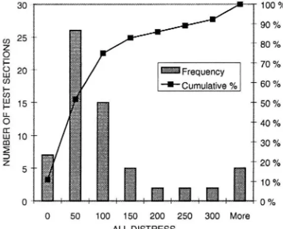
Figure 5 shows the distribution of the total amount of distress for traf c related distress (on wheel paths) and gure 6 all the cracks on a pavement (traffic + climate related), respectively. It can be seen that most of the test sections have cracking. Fifteen test sections do not have traffic related distress and 7 sections show neither traffic nor climate related distress.
30 _ _ ' 100 % - 90 % 25 " -- so %
" ' 70 0/0 Frequency l Cumu|ative % 20 " " 60 %
" 50 % ' 40 % " 30 % NU MB ER OF TE ST SE CT IO NS a: " 20 % ' 10 % _ 0 cyo 0 50 100 150 200 More
TRAFFIC RELATED DISTRESS
Figure 5. Distribution of traffic related
distress on wheel paths (index value).
30 ~ 100 % " 90 0/o (2 25 -_ - 80 % Q.
B
_,
W
- 70 %
& +Cumu|ative % "' 60 % (D L 15 " ;.-:' 50 0/i;
°
g % -- 40 % å 10 " äg): " 30 0/0% 5 _
ååå
- 20 %
få?
låa
10 % 0 _ ' * 0 % 0 50 100 150 200 250 300 More ALL DISTRESSFigure 6. Distribution of traffic + climate
related distress (index value). 5. PAVEMENT RESPONSE
Surface curvature radius and tensile strain at the bottom of the asphalt concrete layer were selected as factors describing pavement behavior under loading. The surface curvature radius is
calculated from the measured FWD de ections as follows (equation 1): 1,2 SCR= (l) D0 __
2 30 ?
where:SCR is the surface curvature radius, m
r is the sensor distance from the center of the loading plate, mm
DO the surface deflection under the loading plate, um
Dr the surface de ection at distance r from the center of the loading plate, um. The distribution of surface curvature radius D90 is shown in figure 7. The average value is 300 meters and most of the values vary between 100 and 600 meters, respectively.
30 ' 100 % " 90 0/o
g 25 __
80 %
(_) Frequency __ o 5 20 +Cumulative % 70 /° % |__ 60 /ofå 15 _
- 50 %
LL O * 40 % 0: _ å 1° - 30 %%
' 20 (Yo z 5 _ _ 10 0/0 O * " 0 % 100 200 300 400 500 600 MoreSURFACE CURVATURE RADIUS
Figure 7. Distribution of surface curvature
radius (m) based on D,=900 mm.
Critical strains are usually longitudinal tensile strain at the bottom of the asphalt layer and vertical compressive strain at the top of the subgrade. Critical strains were calculated with the linear elastic program (BISAR) using the layer moduli values from the Modulus backcalculations and layer thickness from the test pits /4, 5, 6/. Poisson s ratio of u = 0.35 was used for all layers in the calculations /7/.
The backcalculated layer moduli values have a significant effect on strains when linear elastic programs are used for calculations. Obtaining realistic estimates for pavement layer moduli with backcalculation requires experience and knowledge of the backcalculation system. Based on experience, the results are not always easy to
interpret, especially on pavements with thin asphalt bound layers which are typical for pavements used in the study. In order to avoid uncertainties related to the backcalculated moduli values, a new neural network based model was developed in which measured de ection bowl and layer thickness were used as input for strain calculations.
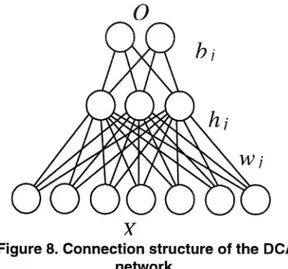
A non-linear neural network model developed by Jokinen was used in the analysis /8/. The model has the ability to estimate the functional form as well as the model parameters simultaneously. The Dynamic Capacity Allocating (DCA) networks have a three layer feed-forward connection structure. Figure 8 shows an example of the network with 7 inputs, 3 hidden nodes and 2 outputs. In this network all outputs from the input layer are connected to all hidden nodes. If the current input pattern vector is _)5, the weights of node i are _vyi and A is a weighting matrix, then the output activation hi of hidden node i is
h
e 261
(2)
where
a is positive scalar constant &, w n*1 column vectors
A positive definite n*n square. The outputs of all hidden nodes hi are used for calculating the jth output of the network Oj
k
01 = Zia-h:-
(3)
i=1 where:
Oj is jth output of the network bij weights of hidden node hi
Figure 8. Connection structure of the DCA network.
The learning process of the DCA network is based on known input and output values. The input data used for teaching the network consisted of simulated pavement thickness and moduli information presented in Table 2. Strains (output data) were calculated for all variable combinations (37:2187) using the BISAR program. Parameters of the model are selected in such a way that the error of the DCA network model response is smaller than the predefined tolerance.
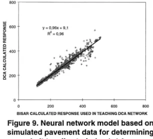
The correlation between BISAR calculated strains and DCA network model strains based on de ection bowl and asphalt layer thickness is shown in figure 9. The learning data for the DCA network consisted of de ection bowl and asphalt layer thickness information.
It can be seen that the neural network model correlates well with BISAR calculated strains. The benefits of using the DCA network model are related to avoiding uncertainties involved in determining moduli values for all pavement layers and subgrade with the backcalculation programs. For this reason DCA strains were used as input in deterioration model development instead of strains derived from backcalculation process combined with output from the linear elastic layer program. Table 2. Simulated input data for DCA network.
ASPHALT CONCRETE BASE SUBBASE SUBGRADE Thickness Modulus Thickness Modulus Thickness Modulus Modu|us
mm MPa mm MPa mm MPa MPa
50 2000 100 200 400 120 20
100 5000 200 280 800 200 1 10
800 O' ) O O y = 0,96x + 9,1 R2 = 0,96 D C A C A L C U L A TE D R E S P O N S E J) O0 N O O O l I | 0 200 400 600 800
BISAR CALCULATED RESPONSE USED IN TEACHING DCA NETWORK
Figure 9. Neural network model based on simulated pavement data for determining
asphalt tensile strain (um/m) from a
deflection bowl measured with FWD.
Deflection bowl and asphalt layer thickness
used as learning data.
6. MODELING APPROACH
A typical feature of road deterioration is that cracking does not occur on a whole pavement at the same time but at different times and at various locations even on a short section of road. Areas where the first cracks appear depend on the variability of traffic (including dynamic loading effects) and climate factors, layer thickness, material characteristics and subgrade properties. Pavement behavior and deterioration is therefore a complicated system where the occurrence of cracking is stochastic by nature. This means that pavements usually have a large variability in failure times which should be taken into account in the development of deterioration models.
Failure time can be defined as a survival time that determines the occurrence of a given event. In this study survival time is the cumulative number of axle loadings to failure. These times are subjected to random variations which form a distribution. The distribution of survival times is usually characterized by three functions /9/:
. probability density function, 0 survival function,
0 hazard function.
The survival (failure) time T has a probability density function de ned as the limit of the probability that a road deteriorates in time interval t to
t + At per unit time width At . It can be expressed
as /9/:
. P DETER
f(t)= hm
()
(4)
At >0
At
where:
DETER is a road deteriorating in the interval (t + At)
The graph of f(t) is called the density curve. Figure 10 illustrates the probability density functions of failure times separately for observed traffic induced distress (on wheel paths) and climate induced distress (outside wheel paths) for test sections (time width is two years). Failure time is defined as the time to the appearance of first crack on pavement surface. It can be seen that for traf c related distress the high frequency of failure occurs when pavement age is around 5 - 7 years. The distribution of climate related distress is more flat and most of the distress occur when pavement age is between 6 and 12 years.
0,4
+CLIMATE"*"TRAFFIC 0,35 """""" ' 0,3 0,25 " f(t ) 0,2 """" 0,15 '" " " 0,1 ' * 0,05 "' AGE (years)
Figure 10. Probability density curves for
traffic and climate induced distress at the
initiation of cracking.
The survival function, S(t), is defined as the probability that a road survives longer (does not meet the distress criteria) than t:
S(t) = P(a road survives longer than t) = P(survival time > t) (5) From the definition of the cumulative distribution function F(t) of the survival time T the following can be written /9/:
S(t) = 1 - P(a road deteriorates before time t)
= 1 - F(t)
(6)
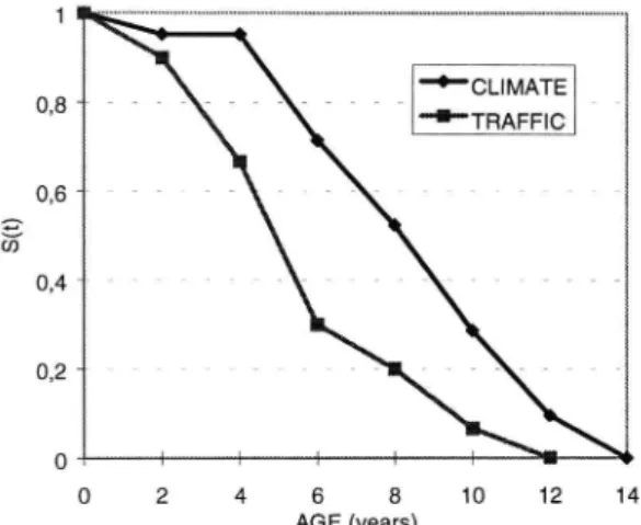
An example of the survival curve is shown in figure 11 for measured data. It can be used to determine the probability that the pavement will last longer than t. For example, it can be seen that traffic
related distresses occur sooner than climate related distresses. The median (50th percentile) age for traffic distress to occur is 5 years and for climate distress 8 years, respectively.
1 ., 08_ _____ , 77777 "'"'CLIMATE * *"TRAFFIC 0,6 - ~
%
,
0,4 ' _ ffffffff og wmf w. O . > o 2 4 6 8 10 12 14 AGE (years)Figure 11. Example of the survival curves.
The hazard function h(t) of survival time T gives the conditional failure rate. This is defined as the probability of failure during a small time interval assuming that the road has survived to the start of the interval. The hazard function can be expressed as /9/:
P AGEDET
h(t) =
lim
(
)
(7)
At >0
Af
where:
AGEDET is a road of age t deteriorating in the time interval (t, t+At)
The hazard function can also be defined in terms of the cumulative distribution function F(t) and the probability density function f(t):
h(t) ___ lg.
(1 F(0)
The hazard function thus gives the risk of failure per unit time during the aging process. Examples of hazard functions for measured traffic and climate related distress are depicted in figure 12. It can be seen that the occurrence of both traffic and climate distress on pavement surface (initiation of cracking) have an increasing risk of failure as pavement age increases.
(8)
2
13" * ' +CLIMATE
1,6 » "'.' TRAFFIC h( t) 12 AGE (years)Figure 12. Hazard functions for traffic and
climate induced distresses (initiation of
cracking).
The location and shape of functions along the time axis t depend on the factors affecting pavement deterioration.
In addition to variability, the different behavior mechanism of non-cracked and cracked pavements should be taken into account in developing deterioration models. This is because the behavior of pavement structure is different depending on the condition of a road. A crack on a pavement surface forms a discontinuity which reduces the capability of an asphalt concrete layer to distribute the traffic load as well as a non-distressed pavement.
Because of the different behavior of non cracked and cracked pavements, the development of pavement deterioration models using a failure time approach should be based on the method which includes two separate phases:
1. Prediction of time to appearance of the first crack.
2. Prediction of time when cracking has progressed to a certain level.
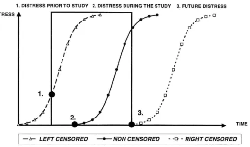
The long-term pavement performance data includes observations which are not complete. This means that there are sections for which the exact life time (failure time) is unknown. These are called censored observations, which must be taken into account in the model development in order to utilize the information they contain. Figure 13 illustrates data collected from the test sections within a certain time period and indicates the left- and right censored data, respectively / 10/.
1. DISTRESS PRIOR TO STUDY 2. DISTRESS DURING THE STUDY 3. FUTURE DISTRESS
DISTRESS A «r- "3
fw QD. .D'D'D
qr ' ..n' ; TIME
I A LEFT CENSORED '_' MON CENSORED ' 'D ' RIGHT CENSORED
Figure 13. Illustration of censored data.
Some of the test sections selected for the study already had distress on the pavement surface. A precise time for the occurrence of cracking is not known prior to the first condition survey. All we know is that these pavements did not last longer than the age (or cumulative number of axle loads) at the first survey. These are referred to as left censored observations because the actual occurrence of distress was earlier (to the left of) than the time at which the distress was first observed.
On the other hand, some test sections have not shown distress during the survey, or they were dropped from the study because of maintenance. In this case we do not know precisely when the distress will appear (or would have appeared) on the pavement surface. All we know is that the pavement has lasted at least this long without a failure or had not failed when the maintenance operations were carried out for other reasons than distress. These observations are known as right-censored because the true time for a failure is to the right of last observed time.
There is not enough data to develop deterioration models if only the exact or uncensored observations (distress occurred during the study) are used as input data. For this reason a statistical method which takes into account stochastic variations and censored data was applied in the data analysis. The SAS procedure LIFEREG was used which fits parametric models to failure time data which can be censored /l 1/. The model for the response variable consists of a linear effect composed of the covariables together with a random disturbance term of which distribution form
is determined by the data. The parameters are estimated by the maximum likelihood method.
The models for the response variable (cumulative traffic to the initiation of cracking) consist of a linear effect composed of the covariables together with the random disturbance term of known distribution.
The model assumed for the response y with n observations is /1 1/:
y=XB+oe
(9)
where:
y is the vector of response values (failure time) X n*k matrix of covariate values (independent variables)
,B the vector of unknown regression parameters O' the unknown scale parameter
8 the vector of errors.
8 is assumed to come from a known distribution with survival distribution function S, cumulative distribution function F and probability density function f. That is S(t) PROB(8i >t), F(t) : PROB(8i <= t) and f(t) dF(t)/dt where El. is a component of the error vector. Then if all the responses are observed (no censored data), the log-likelihood (L) can be written as /11/:
f(Wi)
g __
L = 210
(10)
: (yi _?Ci'B)
O'
If some of the responses are left, right or interval censored, the log-likelihood can be written as /11/:
L= Zlog[f(;vi))+210g(S(Wl-))+
Zlog(F(wi )) + 2 log(F(wl-) _ F(vi))
Wi
(11)
with the first sum over uncensored observations, the second sum over right censored observations, the third sum over left censored observations, the last sum over interval censored observations andvi = (Zi xi' B) / O' where Zi is the lower end of a
censoring interval. The log-likelihood function is maximized by means of a ridge-stabilized Newton-Raphson algorithm.
As it has been illustrated in figure 12 both traffic and climate distress on pavement surface have an increasing risk of failure as pavement age increases. This indicates that the probabilities of traffic (fatigue) and climate (uneven frost heave, oxidation of surfacing) induced distresses are expected to increase as the pavement ages. This can be described as an increasing hazard function (hazard of cracking).
The distribution which models the variation of failure times with increasing risk of failure is Weibull distribution /9/. Its density function (f), survival distribution function (S), and hazard function (h) are as follows:
f (t)=Ä*7*(Å * f)y_1* ( )y
(12>
S(t) = [WN
(13)
h(t) = liq/NAM)?
(14)
where:7 determines the shape of the distribution curve (shape parameter)
Ä determines scaling of the curve (scale parameter).
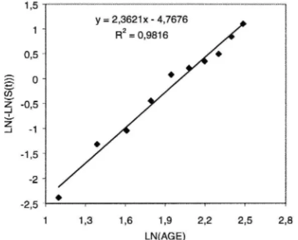
It is possible to determine whether data are generated by a Weibull distribution by producing a graphical plot which shows the relationship between the value of loge(time) and the function loge(-loge(S(t))). If the theoretical distribution is correct, a
straight line can be drawn through the data points. An example of the output is shown in figure 14. The horizontal axis describes the loge of failure time (in years) for the initiation of traffic related cracking (on wheel paths) and the vertical axis is the loge of the negative loge of survival distribution function S(t). S(t) has been determined using SAS procedure LIFETEST /l l/. From the Figure it can be seen that the relationship is linear (R2=O.98) that confirms that Weibull distribution can be selected for data analyses. Further, if the slope and intercept of the plot are a and b, then rough estimates of shape parameter 7 and scale parameter 7». are b and exp(a/b), respectively. Based on data the value of shape parameter is estimated as y = 2.36 and scale parameter 71. = 0.13 /9/. y = 2,3621x - 4,7676 R2 = 0,9816 LN (-LN (S (t )) ) o 01 1 1,3 1,6 1,9 2,2 2,5 2,8 LN(AGE)
Figure 14. Weibull probability plot of survival
time for the initiation of traffic related distress.
7. FAILURE TIME MODELS
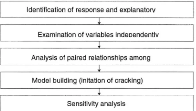
A systematic approach was used in developing deterioration models. Modeling phases applied in the study are shown in figure 15. First, the response (dependent) and explanatory (independent) variables were identified from the data base. Subsequently the data were reviewed and evaluated by examining both response and explanatory variables independently. In order to explore dependencies between two variables, analysis of paired relationships among variables was performed. The development of deterioration models is done in the model building phase.
Identification of response and exolanatorv
l
Examination of variables indeoendentlv
l
Analysis of paired relationships among
l
Model building (initation of cracking)
l
Sensitivity analysis
Figure 15. Flow chart for developing deterioration models.
The explanatory or independent variables used in the analyses consist of information from traffic, climate, pavement structure and subgrade, pavement response, roughness, age and different two factor interactions.
The variables are as follows: . traffic
annual average daily traffic
- annual cumulative number of equivalent single axle loads
proportion of heavy vehicles - climate
average annual freezing index
cumulative freezing index (pavement age*annual freezing index)
average annual rainfall
cumulative rainfall (pavement age*annual rainfall)
0 pavement structure
layer thickness (asphalt concrete, base, sub-base layer)
backcalculated moduli (asphalt concrete, base, sub base layer, subgrade)
all two factor interactions between layer thickness and moduli (thickness*modulus) ' pavement response
measured de ection, bearing capacity measured surface curvature radius
calculated tensile strain at the bottom of the asphalt concrete layer
calculated vertical strain at the top of the subgrade
. roughness IRI . pavement age 0 new variables
cluster variables (various interactions of the above mentioned variables)
Failure time models were developed separately for traffic and the combination of traffic and climate induced distress. Dependent variable is the number of cumulative traffic loadings to the initiation of cracking. In the model development various one, two and three explanatory variable combinations were evaluated as part of the analysis process.
Failure time data regarding the initiation of traffic related cracking consist of observations of which 30 were left censored, 8 right censored and 26 uncensored observations (time of cracking was known), respectively.
Best models for predicting the cumulative number of loadings to failure due to traffic (distress on wheel paths) are based on explanatory variables related to pavement response (strain, surface curvature radius ) and the effect of ageing which is a relationship between a response parameter and the annual cumulative number of traffic loadings.
Equation 15 shows the strain based deterioration model and it is illustrated in figure 16.
6.56 0.003*(ABEUB) 2658469*(A BEU 113* )
N 10 = 10 10
(15)
where:
N10 is cumulative traffic loadings at the initiation of cracking
ABEUB is strain at the bottom of asphalt layer, urn/m
1 200 000
+50000 ESAL/YR ' 100000 ESAL/YR
900 00°
+250000 ESAL/YR
_|E% 600 000 ;
"
300 000 _ "95555 0 : : : 150 200 250 300 350 ABEUBFigure 16. Prediction of cumulative number of axle loadings to failure (distress on wheel
paths) at initiation of cracking as a function of strain ABEUB (um/m) with annual cumulative
traffic 100,000. As figure 16 illustrates, for strong pavements
(strain 150 urn/m) the cumulative number of axle loadings (ESAL) varies between 600,000 and 1,100,000 loadings to the initiation of cracking when annual traffic loadings are between 50,000 and 250,000. For weaker pavements the effect of different annual loading levels on cumulative ESAL is smaller than for strong pavements.
The effect of climate on pavement deterioration was investigated for both traffic and climate related distresses. Failure time data regarding the initiation of
traffic and climate related cracking consist of observations of which 41 were left censored, 3 right censored and 20 uncensored observations (time of cracking was known), respectively.
The results indicate that both surface curvature index and the annual freezing index are important factors explaining deterioration due to cold climate. The model is described in equation 16 the initiation of cracking.
(16)
1288+ 0.0017 * (SCR90) 1.00* (log 10(SCR90) * 10000) 153 * LFROST
N10 = 10 N10Y
where:
N10 is cumulative traffic loadings at the initiation of cracking SCR90 surface curvature radius, m, at the distance of 900 mm LFROST log10(freezing index), h°C
NIOY annual traffic loadings.
The equation 16 is illustrated in figure 17 for various surface curvature radius values when freezing index (FR.IND.) values are 10000, 12000 and 18000 hOC (freezing index has a positive sign in input data for calculation purposes) and traffic loading level (annual cumulative number of axle loads) has been selected for 100,000 ESAL for illustration purposes.
Figure shows that the effect of surface curvature radius on cumulative ESAL is larger on a strong pavement (high SCR90 value) than on a weak pavement. This means that the effect of colder climate has a stronger influence on deterioration on a weak pavement compared to the same effect on a strong pavement as a result of uneven frost heave.
1000000 + : 800000 __ FR.IND. 10000 FR.IND.=12000 +FR.IND.=18000 600000 __| <1: co Lu ... 400000 200000 0 '. 200 300 l l 400 500 600 SCR90
Figure 17. Prediction of cumulative number of axle loadings to failure (both traffic and
climate related distress) at initiation of cracking as a function of surface curvature radius
and freezing index when annual traffic loadings are 100,000.
All the variables in deterioration equations 15-16 are statistically significant. The probability of a chi-square value Pr>Chi equals 0.0001 for all the independent variables and intercept.
CONCLUSIONS
This paper deals with pavement deterioration models that are based on long-term pavement monitoring data from Finland and Sweden. Models have been developed for both traffic and traffic and climate induced distress. The modelling is based on failure time approach that can use censored data in analysis. This is a benefit when only a limited number of sections are available which exact failure time is known.
The models were developed to predict the initiation of cracking as a function of pavement response (strain, surface curvature radius) and climate factor. A neural network model is presented that can be used to calculate tensile strains at the bottom of asphalt layer using measured FWD de ection bowl and thickness of pavement layers.
Deterioration models can be used in a pavement management system to assess how many load applications a pavement can carry before cracking occurs on surface.
The models have been developed using FWD data measured in the summer time. The models will be updated when spring time de ection data is available from the test sections in order to take seasonal variation of pavement response into account in model development.
REFERENCES
1. Nordic SHRP LTTP. Status report. Swedish Road and Transport Research Institute (VTI), Technical Research Centre of Finland (VTT), Danish Road Institute (DRI), Norwegian Road Research Laboratory (NRRL),. September 1995. 2. Distress Identi cation Manual for the Long-Term
Pavement Performance Project. SHRP-P-338. SHRP. Washington D.C. 1993.
3. SHRP-LTPP Manual for FWD Testing. Operational Field Guidelines. Version 1.0, Washington D.C.
1989.
4. Scullion, T., Michalak, C., Modulus 4.0: User s manual. Research Report ] 123-4f. Texas Transportation Institute. College Station, Texas
5. Ruotoistenmäki, A., Jämsä, H., Determination of 9. Lee, E., Statistical Methods for Survival Data Layer Moduli from FWD Measurements. A Case Analysis. A Wiley-Interscience Publication. New Study of 44 Sections. EUROFLEX-European York 1992.
Symposium on Flexible Pavements. Lisbon 1993. 10. Paterson, W., Road Deterioration and 6. Ruotoistenmäki, A., Determination of Layer Moduli Maintenance E ects, Models for Planning and
from Falling Weight Deflectometer Measure- Design. World Bank, 1987.
ments. VTT Research Notes. Technical Research ll. SAS/STAT Guide for Personal Computers. Centre of Finland, Espoo 1994. Version 6 Edition. SAS Institute Inc. 1987. 7. AASHTO Guide for Design of Pavements.
AASHTO. Washington, D.C., 1986.
8. Jokinen, P., Continuously Learning Nonlinear Networks with Dynamic Capacity Allocation. Tampere University of Technology, Publications 73. Tampere 1991.