Mälardalen University Press Dissertations No. 138
PARAMETRIC WCET ANALYSIS
Stefan Bygde
2013
School of Innovation, Design and Engineering Mälardalen University Press Dissertations
No. 138
PARAMETRIC WCET ANALYSIS
Stefan Bygde
2013
Mälardalen University Press Dissertations No. 138
PARAMETRIC WCET ANALYSIS
Stefan Bygde
Akademisk avhandling
som för avläggande av filosofie doktorsexamen i datavetenskap vid Akademin för innovation, design och teknik kommer att offentligen försvaras
tisdagen den 4 juni 2013, 13.00 i Delta, Mälardalens högskola, Västerås. Fakultetsopponent: Principal Lecturer Raimund Kirner, University of Hertfordshire
Akademin för innovation, design och teknik Copyright © Stefan Bygde, 2013
ISBN 978-91-7485-109-0 ISSN 1651-4238
Mälardalen University Press Dissertations No. 138
PARAMETRIC WCET ANALYSIS
Stefan Bygde
Akademisk avhandling
som för avläggande av filosofie doktorsexamen i datavetenskap vid Akademin för innovation, design och teknik kommer att offentligen försvaras
tisdagen den 4 juni 2013, 13.00 i Delta, Mälardalens högskola, Västerås. Fakultetsopponent: Principal Lecturer Raimund Kirner, University of Hertfordshire
Akademin för innovation, design och teknik
Mälardalen University Press Dissertations No. 138
PARAMETRIC WCET ANALYSIS
Stefan Bygde
Akademisk avhandling
som för avläggande av filosofie doktorsexamen i datavetenskap vid Akademin för innovation, design och teknik kommer att offentligen försvaras
tisdagen den 4 juni 2013, 13.00 i Delta, Mälardalens högskola, Västerås. Fakultetsopponent: Principal Lecturer Raimund Kirner, University of Hertfordshire
Abstract
In a real-time system, it is crucial to ensure that all tasks of the system hold their deadlines. A missed deadline in a real-time system means that the system has not been able to function correctly. If the system is safety critical, this could potentially lead to disaster. To ensure that all tasks keep their deadlines, the Worst-Case Execution Time (WCET) of these tasks has to be known.
Static analysis analyses a safe model of the hardware together with the source or object code of a program to derive an estimate of the WCET. This estimate is guaranteed to be equal to or greater than the real WCET. This is done by making calculations which in all steps make sure that the time is exactly or conservatively estimated. In many cases, however, the execution time of a task or a program is highly dependent on the given input. Thus, the estimated worst case may correspond to some input or configuration which is rarely (or never) used in practice. For such systems, where execution time is highly input dependent, a more accurate timing analysis which take input into consideration is desired. In this thesis we present a method based on abstract interpretation and counting of semantic states of a program that gives a WCET in terms of some input to the program. This means that the WCET is expressed as a formula of the input rather than a constant. This means that once the input is known, the actual WCET may be more accurate than the absolute and global WCET. Our research also investigate how this analysis can be safe when arithmetic operations causes integers to wrap-around, where the common assumption in static analysis is that variables can take the value of any integer. Our method has been implemented as a prototype and as a part of a static WCET analysis tool in order to get experience with the method and to evaluate the different aspects. Our method shows that it is possible to obtain very complex and detailed information about the timing of a program, given its input.
ISBN 978-91-7485-109-0 ISSN 1651-4238
Abstract
In a real-time system, it is crucial to ensure that all tasks of the system hold their deadlines. A missed deadline in a real-time system means that the system has not been able to function correctly. If the system is safety critical, this could potentially lead to disaster. To ensure that all tasks keep their deadlines, the Worst-Case Execution Time (WCET) of these tasks has to be known.
Static analysis analyses a safe model of the hardware together with the source or object code of a program to derive an estimate of the WCET. This es-timate is guaranteed to be equal to or greater than the real WCET. This is done by making calculations which in all steps make sure that the time is exactly or conservatively estimated. In many cases, however, the execution time of a task or a program is highly dependent on the given input. Thus, the estimated worst case may correspond to some input or configuration which is rarely (or never) used in practice. For such systems, where execution time is highly input dependent, a more accurate timing analysis which take input into consideration is desired.
In this thesis we present a method based on abstract interpretation and counting of semantic states of a program that gives a WCET in terms of some input to the program. This means that the WCET is expressed as a formula of the input rather than a constant. This means that once the input is known, the actual WCET may be more accurate than the absolute and global WCET. Our research also investigate how this analysis can be safe when arithmetic operations causes integers to wrap-around, where the common assumption in static analysis is that variables can take the value of any integer. Our method has been implemented as a prototype and as a part of a static WCET analysis tool in order to get experience with the method and to evaluate the different as-pects. Our method shows that it is possible to obtain very complex and detailed information about the timing of a program, given its input.
Acknowledgements
This thesis is the result of my research since fall 2006. I like to begin by thanking Bj¨orn Lisper, Hans Hansson and Christer Norstr¨om for deciding to employ me as a PhD student at M¨alardalen University! I am also very grateful to my supervisors Bj¨orn Lisper (my main supervisor), Andreas Ermedahl (co-supervisor for the first few years), and Jan Gustafsson (co-(co-supervisor). I also would like to thank Niklas Holsti whom I have been working together with a lot the recent couple of years. Thank you all very much!
I have been meeting a lot of people during these years and have got a lot of new friends and had a lot of good times. I would like to thank all my colleagues, friends and family. I will not attempt to make a list of all people that deserves my gratitude during these years, but if you are looking for your name here it means that you have my thanks! Thank you very much for your support!
My research has been funded by CUGS (the National Graduate School in Computer Science, Sweden), the Swedish Foundation for Strategic Research (SSF) via the strategic research centre PROGRESS and finally by the Marie
Curie IAPP project APARTS.
Stefan Bygde V¨aster˚as, May, 2013
Contents
1 Introduction 1
1.1 Embedded Systems . . . 1
1.2 Real-Time Systems . . . 2
1.3 Worst-Case Execution Time . . . 2
1.3.1 Determining the WCET of a Program . . . 3
1.4 WCET Analysis . . . 4
1.4.1 Dynamic Analysis . . . 4
1.4.2 Static Analysis . . . 5
1.4.3 Relation between approaches and the WCET . . . 5
1.5 Static WCET Analysis . . . 6
1.5.1 Flow Analysis . . . 7
1.5.2 Low-Level Analysis . . . 8
1.5.3 Calculation . . . 9
1.6 Parametric WCET Analysis . . . 10
1.6.1 Benefits of Parametric WCET Analysis . . . 11
1.6.2 Related Work . . . 12
1.7 Summary . . . 14
2 Research 15 2.1 Introduction and Background . . . 15
2.2 Research Method . . . 16
2.3 Problem Formulation . . . 16
2.4 Overview of Solutions . . . 17
2.4.1 Approach to Research Questions . . . 17
2.4.2 Contributions . . . 18
2.4.3 Summary of Publications . . . 19
2.5 Thesis Outline . . . 20 vii
viii Contents
3 Technical Introduction 23
3.1 Notation and Conventions . . . 23
3.1.1 Functions . . . 23 3.2 Program Model . . . 24 3.2.1 Syntax . . . 25 3.2.2 Semantics . . . 27 3.2.3 Example . . . 30 3.2.4 Program Timing . . . 31 3.3 Traces . . . 31 3.3.1 Trace Semantics . . . 33
3.3.2 Using Trace Semantics to Compute the Execution Time 33 3.4 Parametric WCET Analysis . . . 34
3.4.1 Making it a Counting Problem . . . 35
3.5 Collecting Semantics . . . 39
3.6 Control Variables . . . 40
3.7 Input Parameters . . . 44
3.7.1 Representing Programs . . . 48
3.8 Summary . . . 50
4 Abstract Interpretation and the Polyhedral Domain 51 4.1 Domain Theory . . . 51
4.1.1 Lattices . . . 52
4.1.2 Fixed Point Theory . . . 53
4.2 Introduction to Abstract Interpretation . . . 54
4.2.1 Abstraction . . . 54
4.2.2 Abstract Functions . . . 56
4.2.3 Widening and Narrowing . . . 58
4.3 The Polyhedral Domain . . . 59
4.3.1 Convex Polyhedra . . . 60
4.3.2 Representation . . . 60
4.3.3 The Lattice of Convex Polyhedra . . . 61
4.3.4 Convex Polyhedra as Abstract Domain . . . 63
4.4 Approximating Program Semantics . . . 64
4.4.1 The Polyhedral Domain as Abstract Environment . . . 65
4.4.2 The Abstract Semantic Function . . . 66
4.5 Abstract Interpretation Example . . . 68
Contents ix 5 Parametric WCET Analysis 71 5.1 Introduction . . . 71
5.2 Overview . . . 71
5.3 The State Counting Phase . . . 72
5.3.1 Preparing the Program . . . 73
5.3.2 Relational Abstract Interpretation . . . 74
5.3.3 State Counting . . . 74
5.3.4 Example of the State Counting Phase . . . 77
5.4 The Parametric Calculation Phase . . . 79
5.4.1 Parametric Integer Programming . . . 80
5.5 Reducing the Number of Variables . . . 82
5.5.1 Concrete Example of Variable Reduction . . . 84
5.5.2 The Minimum Propagation Algorithm . . . 86
5.6 The Combination Phase . . . 87
5.7 Simplification . . . 87
5.8 Summary . . . 89
6 The Minimum Propagation Algorithm 91 6.1 Introduction . . . 91
6.2 The Minimum Propagation Algorithm . . . 91
6.2.1 The Min-Tree . . . 93 6.2.2 The Algorithm . . . 93 6.2.3 Example of MPA . . . 96 6.3 Properties of MPA . . . 99 6.3.1 Termination . . . 99 6.3.2 Complexity . . . 101 6.3.3 Correctness of MPA . . . 101
6.3.4 Upper Bounds on Tree Depth . . . 103
7 Fully Bounded Polyhedra 105 7.1 Analysis on Low-level Code . . . 105
7.2 Representing Integers . . . 107
7.3 Introduction and Related Work . . . 107
7.4 Simon and King’s Method . . . 108
7.4.1 Implicit wrapping . . . 109
7.4.2 Explicit Wrapping . . . 109
7.5 Fully Bounded Polyhedra . . . 110
7.6 Motivation and Illustrating Example . . . 110
x Contents
7.6.2 Making Polyhedra Bounded . . . 115
7.6.3 Making Widening Bounded . . . 116
8 Implementation 119 8.1 Introduction . . . 119
8.2 First Prototype . . . 119
8.2.1 Input Language . . . 119
8.2.2 Implemented Analyses . . . 120
8.2.3 Discoveries and Experience . . . 121
8.3 SWEET . . . 122
8.3.1 Implemented Analyses . . . 122
8.3.2 Discoveries and Experiences . . . 123
9 Evaluation 125 9.1 Introduction . . . 125
9.1.1 Benchmarks . . . 125
9.1.2 A Note on Input Parameters . . . 128
9.1.3 Experimental set-up . . . 128
9.2 Evaluating Parametric Calculation . . . 128
9.2.1 Evaluation of Precision . . . 130
9.2.2 Evaluation of Upper Bounds on Min-Tree Depth . . . 130
9.2.3 Scaling Properties . . . 133
9.3 The Reason for Over-Estimation . . . 135
9.4 Evaluation of Bounded Polyhedra . . . 137
9.4.1 Comparison between SK and BD . . . 138
9.4.2 Computing the Set of Integers of a Polyhedron . . . . 138
9.4.3 The Results . . . 139
9.4.4 On Efficiency . . . 141
9.5 Demonstration of Parametric WCET Analysis . . . 142
10 Conclusions 145 10.1 Introduction . . . 145
10.2 Research Process . . . 145
10.3 Main Results . . . 146
10.3.1 Parametric WCET Analysis . . . 146
10.3.2 Parametric Calculation . . . 147
10.3.3 Analysis of Fixed Size Integers . . . 148
10.4 Future Work . . . 149
10.4.1 Evaluation . . . 149
Contents xi 10.4.2 Analysis on Low-level Code . . . 149
10.4.3 Slicing Techniques . . . 150
10.4.4 Abstract Domains . . . 150
10.4.5 The Minimum Propagation Algorithm . . . 150
Chapter 1
Introduction
In this thesis, we present research with the aim of obtaining safe, input-sensitive estimations of the worst-case execution time of real-time tasks in embedded systems. This introductory chapter explains what this means and puts it into context.
1.1 Embedded Systems
Computer systems which are designed for a specific purpose and which are not operated using a mouse and keyboard like a regular PC are usually referred to as embedded systems. Embedded systems are in fact the most common type of computer systems we use today since they are integrated into mobile phones, cars, trains, aeroplanes, toys, industrial robots etc. Since these systems are specialised in performing specific tasks, and are part of the internal electronics of devices or vehicles, they typically have different requirements than PCs. Often they are small, battery driven and may have strict requirements on safety, performance, energy consumption or timing. In general, embedded systems are more resource constrained than PCs. Most PCs today run on 32-bit or 64-bit processors, while a large portion of embedded systems still uses 8-bit or 16-bit processors.
2 Chapter 1. Introduction
1.2 Real-Time Systems
A very common characteristic of embedded systems is that they need to be pre-dictable in their timing. This is especially the case in safety critical systems. When the timing is so important in a system that it is not considered to operate correctly if it does not perform its computation within a given time frame, we refer to it as a real-time system or RTS. An RTS has requirements to deliver results within a given time frame as part of its functional specification. Exam-ples of real-time systems are control systems in cars or aeroplanes, in which the timing is essential and in which case a timing failure actually could result in a catastrophe. This thesis focuses on important problems and challenges concerning real-time embedded systems.
Since timing is such a central role in an RTS, a real-time operating system must make sure that all timing constraints are fulfilled. An RTS manages a set of software tasks. A task is a piece of software designed to perform a particular action, or sequence of actions, at a particular time or times. Tasks are commonly executed periodically on the system (i.e., with a constant inter-arrival time). Some tasks, however, are executed aperiodically, often as a result of an external event. To make sure that all tasks, both periodic and aperiodic, respect their timing constraints they have to be scheduled.
To schedule a set of tasks, each task is associated with a set of properties and requirements, such as inter-arrival time (if periodic), execution time, pri-ority and deadline. The real-time system is equipped with a scheduler that at-tempts to make sure that every task can execute, and to make sure it finishes its execution before its deadline (which comes from system requirements) while minimising the consumption of system resources. Some schedulers allow tasks to be interrupted. In such schedulers a task may be suspended to let another task with higher priority execute for a while, as long as the original deadline is still respected. More information about real-time systems and scheduling can be found in, for example [20].
1.3 Worst-Case Execution Time
To make a feasible schedule and make sure all deadlines are met, it is important for the scheduler to know the execution time of a task. The execution time is defined as the time passed between a task starts its execution until it finishes, assuming it is uninterrupted.
The execution time of a task running on a fixed platform will typically vary.
1.3 Worst-Case Execution Time 3 The execution time is affected by the hardware state as well as the input to the task. To make sure that enough time is allocated for a task to execute to its completion, it is essential to know the longest possible execution time a task can have, known as the Worst-Case Execution Time (WCET).
While the terms execution time and WCET are mostly used in the context of tasks in real-time systems, the concepts are applicable to any code segment or program. In the rest of the thesis, we will refer to the WCET and execution times of programs in general, rather than using the specific term task.
1.3.1 Determining the WCET of a Program
Determining the WCET of a program is far from trivial. The worst-case execu-tion time in practice corresponds to a single execuexecu-tion taking the longest time due to the input to the program and the conditions of the hardware. These ex-act conditions are hard to determine due to the complex interex-action of software and hardware. Even small embedded systems may be equipped with advanced and unpredictable (timing wise) hardware features such as caches, pipelines or branch predictors. These features affect the execution times depending on their internal states and interacting with each other in a very complex manner. How-ever, the software has even more impact on the execution time. A non-trivial program typically has a very large number of possible execution paths. The number of paths comes from loops and branches in a program. Finding the sin-gle path that gives the longest possible execution time is not easy. Moreover, which path is executed depends, often in non-trivial ways, on the input given to the program. In summary, finding the execution that takes the longest to execute on a particular platform is not practically possible in the general case, let alone finding the execution time of it (as a consequence of Turing’s Halting problem).
The practical approach to determine the execution time of a program is to
estimate the WCET as close as possible. To be absolutely sure that the deadline
cannot be missed, this estimate has to be safe, meaning that it has to be at least as large as the actual WCET. However, if the allocated execution time of a program is much longer than the actual WCET, it means that the scheduler is making an unnecessarily inefficient schedule. In the worst case, a too long execution time estimate may cause the program set not to be schedulable at all! This means that the estimation should be as precise as possible while remaining safe. This is very challenging, and as we will see, there are several approaches to make such an estimate.
4 Chapter 1. Introduction
1.4 WCET Analysis
WCET analysis is a systematic process dedicated to obtain an estimate of the WCET of a program. Under certain conditions, such an estimate can be guar-anteed to be safe. Figure 1.1 outlines the relationship between execution times and safe estimates. The figure also displays the sometimes important concept of Best-Case Execution Time (BCET), which is defined exactly as WCET but refers to the shortest possible execution time of a program.
probability
actual WCET actual
BCET
The actual WCET must be found or upper bounded
time possible execution times
0 lower timing bound upper timing bound timing predictability worst-case performance worst-case guarantee
Figure 1.1: Relation between execution times and analysis results (taken from [119])
Thus, any number greater than or equal to WCET is a safe estimate, but to avoid impossible or impractical schedules this estimate should naturally be as small as possible while being safe. Quite a lot of research has been dedicated to the field of WCET analysis. A good introduction can be found in [119]. There are several approaches to obtaining WCET estimates, but they can in general be classified as dynamic, static or hybrid approaches.
1.4.1 Dynamic Analysis
Dynamic (or measurement based) approaches, which have long been the indus-trial standard, are methods that rely on running or simulating a program to find information about the execution time. In order to find the WCET then, the pro-gram would have to be run on its worst-case input and its worst-case hardware state. However, it is typically very difficult to know which is the worst-case in-put and hardware state. Thus, the dynamic approach has to execute a program end-to-end a large number of times with a large number of inputs and observe
1.4 WCET Analysis 5 the longest execution time. However, unless it is a very simple program run-ning on very simple hardware, the measured executions will constitute a subset of the actual set of possible executions. Thus, there are no guarantees that the worst-case has been observed. This means that results from measurement based approaches typically cannot be considered as safe estimates. To compen-sate for this, sometimes a safety margin is added to increase the likelihood of safety [103]. However, it should be noted that the longest observed execution time constitutes a lower bound for the WCET, which may be a useful indicator of the accuracy of a safe estimate obtained by another method.
Methods for measuring the execution time are outlined in [108]. The sim-plest way is to simply measure end-to-end execution time using something as simple as a stop-watch (for very coarse approximations) or the time com-mand in Unix. More sophisticated approaches may include the use of profiling or dedicated software analysers.
1.4.2 Static Analysis
Static analysis methods attempt to obtain a WCET estimate without executing or simulating a program. Instead, an estimation is made by statically analysing the software together with the hardware. Static analysis most often aims to derive safe estimates, in contrast to dynamic analyses. However, due to the complexity of software and hardware, and due to the requirement on safety, a static safe static analysis occasionally has to introduce safe approximations re-sulting in a less precise estimate. Often such approximations arise from simpli-fications, with the result that the analysis considers potential executions which actually never occur in the program.
1.4.3 Relation between approaches and the WCET
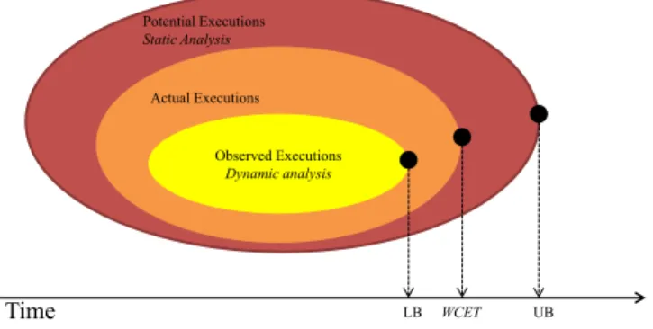
As can be seen, the dynamic and static approaches to WCET analysis do not deliver the same kind of result. Although both aim to derive precise estimates of the WCET, they provide lower and upper bounds of the actual WCET. Fig-ure 1.2 illustrates this concept in a Venn diagram. While this is a bit simplified, it illustrates the basic relationship between the approaches.
There are also hybrid approaches combining static and dynamic analysis. Typically this is done by extracting safe flow information from static WCET analysis and combine it with measured times from traces in some way. Such approaches can generally not guarantee that the result is a lower or upper bound on the WCET, but may provide accurate estimates. Kirner et. al. [69] does this
4 Chapter 1. Introduction
1.4 WCET Analysis
WCET analysis is a systematic process dedicated to obtain an estimate of the WCET of a program. Under certain conditions, such an estimate can be guar-anteed to be safe. Figure 1.1 outlines the relationship between execution times and safe estimates. The figure also displays the sometimes important concept of Best-Case Execution Time (BCET), which is defined exactly as WCET but refers to the shortest possible execution time of a program.
probability
actual WCET actual
BCET
The actual WCET must be found or upper bounded
time possible execution times
0 lower timing bound upper timing bound timing predictability worst-case performance worst-case guarantee
Figure 1.1: Relation between execution times and analysis results (taken from [119])
Thus, any number greater than or equal to WCET is a safe estimate, but to avoid impossible or impractical schedules this estimate should naturally be as small as possible while being safe. Quite a lot of research has been dedicated to the field of WCET analysis. A good introduction can be found in [119]. There are several approaches to obtaining WCET estimates, but they can in general be classified as dynamic, static or hybrid approaches.
1.4.1 Dynamic Analysis
Dynamic (or measurement based) approaches, which have long been the indus-trial standard, are methods that rely on running or simulating a program to find information about the execution time. In order to find the WCET then, the pro-gram would have to be run on its worst-case input and its worst-case hardware state. However, it is typically very difficult to know which is the worst-case in-put and hardware state. Thus, the dynamic approach has to execute a program end-to-end a large number of times with a large number of inputs and observe
1.4 WCET Analysis 5 the longest execution time. However, unless it is a very simple program run-ning on very simple hardware, the measured executions will constitute a subset of the actual set of possible executions. Thus, there are no guarantees that the worst-case has been observed. This means that results from measurement based approaches typically cannot be considered as safe estimates. To compen-sate for this, sometimes a safety margin is added to increase the likelihood of safety [103]. However, it should be noted that the longest observed execution time constitutes a lower bound for the WCET, which may be a useful indicator of the accuracy of a safe estimate obtained by another method.
Methods for measuring the execution time are outlined in [108]. The sim-plest way is to simply measure end-to-end execution time using something as simple as a stop-watch (for very coarse approximations) or the time com-mand in Unix. More sophisticated approaches may include the use of profiling or dedicated software analysers.
1.4.2 Static Analysis
Static analysis methods attempt to obtain a WCET estimate without executing or simulating a program. Instead, an estimation is made by statically analysing the software together with the hardware. Static analysis most often aims to derive safe estimates, in contrast to dynamic analyses. However, due to the complexity of software and hardware, and due to the requirement on safety, a static safe static analysis occasionally has to introduce safe approximations re-sulting in a less precise estimate. Often such approximations arise from simpli-fications, with the result that the analysis considers potential executions which actually never occur in the program.
1.4.3 Relation between approaches and the WCET
As can be seen, the dynamic and static approaches to WCET analysis do not deliver the same kind of result. Although both aim to derive precise estimates of the WCET, they provide lower and upper bounds of the actual WCET. Fig-ure 1.2 illustrates this concept in a Venn diagram. While this is a bit simplified, it illustrates the basic relationship between the approaches.
There are also hybrid approaches combining static and dynamic analysis. Typically this is done by extracting safe flow information from static WCET analysis and combine it with measured times from traces in some way. Such approaches can generally not guarantee that the result is a lower or upper bound on the WCET, but may provide accurate estimates. Kirner et. al. [69] does this
6 Chapter 1. Introduction
Figure 1.2: Relation between WCET Analysis approaches. LB and UB stands for lower bound and upper bound respectively.
by automatically deriving appropriate test-data for which to make measure-ments on. A probabilistic approach is used in [16] which attempts to make a very accurate bound on the WCET with a high probabilistic guarantee of safety.
1.5 Static WCET Analysis
Static WCET Analysis is an emerging technique in industry and there are some commercial static analysis tools on the market such as aiT1and Bound-T2. In
addition to commercial WCET tools there are also WCET tools developed in academia, such as SWEET3, TuBound4and OTAWA5.
The main benefits of using static analysis are:
• It can provide a safe upper bound of the WCET.
• Does not require measuring devices or a controlled environment. • Typically shorter analysis times compared to dynamic analysis. 1http://www.absint.com/ait/
2http://www.bound-t.com/
3http://www.mrtc.mdh.se/projects/wcet/sweet/index.html 4http://costa.tuwien.ac.at/tubound.html
5http://www.otawa.fr/
1.5 Static WCET Analysis 7
• Typically simpler set-up and easier configuration than dynamic analysis. • Can be made partly or fully automated.
In addition, static analysis has a lot of interesting research challenges, such as making the analysis as accurate, fast and automatic as possible. For these rea-sons the research presented in this thesis is focused entirely on static analysis.
Figure 1.3: Relation between analysis phases
Most static analyses are using the same underlying principles, and are es-sentially divided into three independent phases. To put it simply, the flow-analysis phase analyses the software, the low-level flow-analysis phase analyses the hardware and the calculation phase combines the analysis results to calculate an estimation of the WCET. This estimation is in most cases expressed as clock cycles, milliseconds or microseconds. Figure 1.3 shows how the different anal-ysis phases relate.
Our research is concerned mainly with the flow analysis and calculation phases. A low-level analysis is important, but in this thesis, the assumption is that a low-level analysis is available and that it can give timing estimates of atomic parts of a program.
1.5.1 Flow Analysis
Flow analysis (or high-level analysis) analyses the source or object code of a program. The goal of this process is to find constraints on the program that originates from the structure and semantics of the program. Below are given some examples of what type of constraints that a flow-analysis can derive. Structural Constraints. The structure of a program imposes restrictions on
the order and frequency of the execution of different parts of a program. By analysing the graph structure of the program, such constraints can be
8 Chapter 1. Introduction
extracted. When analysing low-level code, this graph structure has to be reconstructed by analysis.
Value Constraints. Value analysis can be used to find information about the set of values that variables can attain during execution. This valuable in-formation can be used to find loop bounds, to find out memory addresses or pointer sets. Perhaps the most popular way of doing value analysis is to use abstract interpretation [34].
Infeasible Paths. The graph structure of a program often has many possible paths through it. In many cases, however, it is not possible for a pro-gram to execute all different paths through the graph. A simple example is an if-statement that is followed by an if-statement with the opposite condition making it impossible to take both if-branches. Detecting such restrictions on the program flow can help to make better estimations of the WCET. Infeasible path detection has been of great interest in litera-ture; Alternbernd [5] explores it by path enumeration, path pruning and symbolic evaluation, in [51] by using abstract execution. Other relevant literature include [109, 71, 61, 4].
Loop Bounds. In order to get a finite upper bound on the WCET, an upper bound on every loop of the analysed program has to be known. Because of this a loop bound analysis is crucial for any WCET analysis, and if a loop bound cannot automatically be derived, it has to be provided by the user. Some approaches on finding loop bounds are identifying loop counters [58, 81, 64] or by abstract interpretation to discover the iteration-space and count the number of points in it [78, 42].
1.5.2 Low-Level Analysis
The low-level analysis analyses a mathematical model of the hardware plat-form. The model should be as detailed as possible, but it has to be conservative, that is, it has to over-estimate rather than under-estimate the possible execution times and hardware states. The purpose of the low-level analysis is to derive worst-case execution times for atomic parts of the program. The atomic parts are usually the instructions or basic blocks of a program.
For a low-level analysis to be accurate, it needs to be taking the timing effects of the advanced features of the hardware into consideration. This may include cache memories, pipelines, branch-predictors etc. This makes
low-1.5 Static WCET Analysis 9 level analysis quite difficult and ultimately the worst-case timing might depend on the entire execution history.
Cache Analysis. An accurate low-level analysis has to account for the effect that a cache has on the WCET. An accurate model should be able to conservatively predict cache misses. Some approaches to cache analysis are found in [44, 40].
Pipeline Analysis. Most modern processors uses a pipeline mechanism to make it possible for instructions to execute in parallel. However, due to pipeline hazards it cannot be assumed that a pipeline is fully utilised at all times. A good low-level analysis must be able to analyse the worst-case effect of the timing that the pipeline can have. Pipeline analysis has been in-vestigated in for example [39, 102, 40].
Branch Predictors. Branch predictors are used to fetch and execute code be-fore a branch is taken. This is so that the pipeline can be utilised even before a conditional branch has been evaluated. A branch predictor may speed up the execution time in average, but a miss-prediction means that the pipeline has to be flushed and to fetch the correct instructions. A good low-level analysis should be able to estimate the effect of this. Ap-proaches to branch predictor analysis are suggested in [32, 83, 84, 39]. Ideally, a low-level analysis should account for several of these effects at the same time, examples of integrated approaches to low-level analysis can be found in [40, 60, 59, 107].
1.5.3 Calculation
When flow facts have been derived from the flow analysis and atomic worst-case execution times have been calculated by the low-level analysis, the results can be combined to obtain a concrete bound of the WCET. This is done in the calculation phase. There are three main approaches to calculation, described below.
Path Based. Path based calculation involves explicitly modeling each path through a loop in order to determine the most costly one. Since each path is analysed it makes it easy to take hardware dependencies be-tween instructions into consideration. Path based calculation is used in [59, 107, 98, 40].
10 Chapter 1. Introduction
Tree Based. This type of calculation uses the syntax-tree of a program as model for the timing. A timing is determined for each node of the tree bottom-up and different rules depending on what the structure that the node represent are used to calculate the timing of the parent node. The first tree-based approach is known as a “timing schema” [90]. Newer approaches to tree-based calculation include [75, 93, 31].
Implicit Path Enumeration. The Implicit Path Enumeration Technique (IPET) was introduced in [73, 74] and a similar method in [97]. The idea here is to represent all path implicitly in contrast to path based calculation that consider paths implicitly. This is done by modeling the execution times for each atomic part of the program and model it as an optimi-sation problem, in particular a linear integer programming problem that is optimised subject to the flow-constraints. This problem is the solved by a linear integer programming solver. This approach has been used in [40, 97, 89]. A parametric IPET method is investigated in Section 5.4.
1.6 Parametric WCET Analysis
It is very common for a program’s execution time to vary according to the given input, often in a complex and unpredictable way. The main reason for this is that the program executes different paths depending on the given input. The worst-case path of a program may correspond to an input that is unlikely or never given to the program, and may not be useful in practice. Thus, if the input would be known, then the worst-case execution time for that particular input would be safe and more precise than the global WCET.
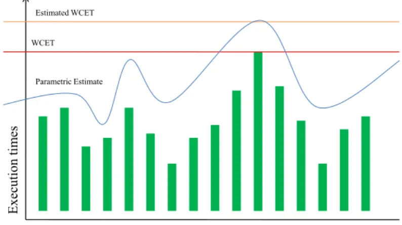
We define a Parametric WCET Analysis to be a WCET analysis which re-sults in a formula rather than a constant. This formula has some selected input as parameters and the formula can be instantiated with concrete values once the input is known. The usefulness of this concept is illustrated in Figure 1.4. The X-axis represents different input combinations that result in different ex-ecution times of a certain program. The red line represents the WCET of the program. The orange line represents a safe upper bound of the WCET which has been obtained by static analysis. A parametric WCET analysis will result in a formula in terms of input. The blue line represents the parametric WCET estimate. As can be seen, the parametric formula gives a safe upper bound of the execution times based on the input. This means that if the input is known, a much smaller (i.e., better!) estimation can be used. As can be seen, the
1.6 Parametric WCET Analysis 11 blue line can even dip below the actual WCET of the program. This is safe, however, if the input is known.
Figure 1.4: Relation between the WCET, a fixed WCET estimation and a para-metric WCET estimation
1.6.1 Benefits of Parametric WCET Analysis
Static WCET analysis is a complex and often time consuming process. If a program would be analysed for every input combination to give a more precise estimate, this would be a very long and tedious process. The benefit of having a formula is that instantiating is much faster than re-analysing a program. A parametric analysis only needs to be done once, and then the formula can be instantiated once the input is known. If the formula is very quick to instantiate, the results could potentially be used in an on-line scheduler where the input is known in advance.
Another benefit of parametric WCET analysis is that it relaxes the require-ment of statically determining concrete upper bounds for each loop in a pro-gram. A concrete WCET estimate is a finite number which depends on upper loop bounds, however, a parametric formula does not need to have a maximum value. If a loop bound is dependent only on parameters, the loop will be bound once the formula has been instantiated. However, if a loop bound is dependent on non-parameters only, the loop bound still has to be statically known.
10 Chapter 1. Introduction
Tree Based. This type of calculation uses the syntax-tree of a program as model for the timing. A timing is determined for each node of the tree bottom-up and different rules depending on what the structure that the node represent are used to calculate the timing of the parent node. The first tree-based approach is known as a “timing schema” [90]. Newer approaches to tree-based calculation include [75, 93, 31].
Implicit Path Enumeration. The Implicit Path Enumeration Technique (IPET) was introduced in [73, 74] and a similar method in [97]. The idea here is to represent all path implicitly in contrast to path based calculation that consider paths implicitly. This is done by modeling the execution times for each atomic part of the program and model it as an optimi-sation problem, in particular a linear integer programming problem that is optimised subject to the flow-constraints. This problem is the solved by a linear integer programming solver. This approach has been used in [40, 97, 89]. A parametric IPET method is investigated in Section 5.4.
1.6 Parametric WCET Analysis
It is very common for a program’s execution time to vary according to the given input, often in a complex and unpredictable way. The main reason for this is that the program executes different paths depending on the given input. The worst-case path of a program may correspond to an input that is unlikely or never given to the program, and may not be useful in practice. Thus, if the input would be known, then the worst-case execution time for that particular input would be safe and more precise than the global WCET.
We define a Parametric WCET Analysis to be a WCET analysis which re-sults in a formula rather than a constant. This formula has some selected input as parameters and the formula can be instantiated with concrete values once the input is known. The usefulness of this concept is illustrated in Figure 1.4. The X-axis represents different input combinations that result in different ex-ecution times of a certain program. The red line represents the WCET of the program. The orange line represents a safe upper bound of the WCET which has been obtained by static analysis. A parametric WCET analysis will result in a formula in terms of input. The blue line represents the parametric WCET estimate. As can be seen, the parametric formula gives a safe upper bound of the execution times based on the input. This means that if the input is known, a much smaller (i.e., better!) estimation can be used. As can be seen, the
1.6 Parametric WCET Analysis 11 blue line can even dip below the actual WCET of the program. This is safe, however, if the input is known.
Figure 1.4: Relation between the WCET, a fixed WCET estimation and a para-metric WCET estimation
1.6.1 Benefits of Parametric WCET Analysis
Static WCET analysis is a complex and often time consuming process. If a program would be analysed for every input combination to give a more precise estimate, this would be a very long and tedious process. The benefit of having a formula is that instantiating is much faster than re-analysing a program. A parametric analysis only needs to be done once, and then the formula can be instantiated once the input is known. If the formula is very quick to instantiate, the results could potentially be used in an on-line scheduler where the input is known in advance.
Another benefit of parametric WCET analysis is that it relaxes the require-ment of statically determining concrete upper bounds for each loop in a pro-gram. A concrete WCET estimate is a finite number which depends on upper loop bounds, however, a parametric formula does not need to have a maximum value. If a loop bound is dependent only on parameters, the loop will be bound once the formula has been instantiated. However, if a loop bound is dependent on non-parameters only, the loop bound still has to be statically known.
12 Chapter 1. Introduction
Having a mathematical formula as estimate can also be beneficial for sev-eral reasons: formulae can be algebraically manipulated, mathematically anal-ysed to find minima and maxima (under certain conditions), evaluated partially, finding timing sensitivity in input etc.
This thesis investigates the concept of parametric WCET analysis and the research aims to make advances in this particular field. Parametric WCET anal-ysis is naturally more complex than classical static WCET analanal-ysis and prob-ably cannot be used on large systems with millions of lines of code; rather, the parametric estimation is most efficiently used on code segments, like small programs or functions, which have input-dependent execution times. Inter-esting applications would include disable interrupt sections, which are code sections which may not be interrupted and are therefore naturally interesting objects for WCET analysis. These sections typically need to be small and are interesting candidates for a parametric WCET [28]. Another important appli-cation of parametric WCET analysis would be in component based software development [36, 62]. In component based software development, reusable components designed to interact with each other in different contexts can be analysed in isolation. Since components are designed to function in different contexts (which would imply different input), a context-dependent WCET es-timate is desired. Component models designed for embedded systems (such as saveCCM [57] or Rubus6) typically use quite small components which makes
parametric WCET analysis interesting.
1.6.2 Related Work
This section presents previous work that is related to parametric WCET anal-ysis in general. One approach to parametric WCET analanal-ysis is to analyse pro-grams parametrised in loop bounds rather than input-values. Vivancos et. al. presents such an analysis in [116], later extended by Coffman et. al [30] for computing polynomial expressions for nested loops. While the method in [116] aims for an integrated cache-analysis which works on low-level code rather than source level code, the flow analysis only takes structural constraints and loop-bound constraints into consideration.
Previous parametric methods has mainly been using path-based or tree-based calculation methods which typically requires that the analysed program has structured program flow [31, 65]. Colin and Bernat [31] uses a tree-based technique with the additional possibility to express constraints such as infeasi-ble paths.
6http://www.arcticus-systems.com/
1.6 Parametric WCET Analysis 13 Some of these approaches [31, 15] relies on using external software like Matlab or Mathematica to simplify and evaluate the parametric formulae. While this is an interesting approach, this is not something that we have explored, but would potentially be interesting.
Many approaches require or recommends user annotations [15, 31] to fully utilise the analysis, while we are aiming to do a fully automatic analysis, ideally without interaction from the user. Some methods [65, 116] are aiming to obtain as simple formulae as possible in order to be able to evaluate them quickly at run-time. This means that these methods intentionally aims to derive a simple (and therefore potentially less precise) formula than possible.
Marref [80] introduces a hybrid approach to parametric analysis based on genetic algorithms. Since part of the method is based on measurements, it cannot be guarantee safety.
In [112], van Engelen et. al. analyses the WCET of loops parametri-cally. It does so by counting points symbolically over the iteration-space of (possibly nested loops) where each iteration of any loop is allowed to have different worst-case timing. However, it assumes that loops are on the form for i = a to b step s, although some of these symbols may be para-metric, it still requires the iteration space has a known form.
Altmeyer et. al. [6] presents a method which is similar to ours: it gives a parametric result in terms of input to the program, uses abstract interpretation to determine values and uses parametric integer programming as calculation method. This method is integrated with cache analysis in order to give precise results for complex architectures. However, this method uses a simpler value analysis that does not take complex linear dependencies between variables into account.
Other interesting approaches of representing properties of programs para-metrically include [3] where the resource cost of executing a program is mod-elled as a recurrence relation and evaluated into closed-form. Gulwani investi-gates how to derive symbolic complexity bounds of a program in [47].
Common for the previous approaches is that they uses mostly constraints coming from program structure, infeasible path information, user annotations, loop bounds (either automatically derived or as information from the user) and except in [65, 6] no automatic value analysis is used to obtain a parametric WCET. Huber et. al. [65] uses SWEET to extract flow facts which uses a non-relational value analysis to derive the constraints.
What differs our method from the previously mentioned methods is that our method do not require structured flow, it does not need to identify loops or other structures explicitly, it parametrises in input-values and is fully
![Figure 1.1: Relation between execution times and analysis results (taken from [119])](https://thumb-eu.123doks.com/thumbv2/5dokorg/4680337.122478/20.718.123.564.336.502/figure-relation-execution-times-analysis-results-taken.webp)


![Table 3.1 shows how the execution time of the trace T 0 of L (see Figure 3.2) starting with input σ 0 = [i �→ 0][n �→ 2] is computed](https://thumb-eu.123doks.com/thumbv2/5dokorg/4680337.122478/50.718.108.576.178.454/table-shows-execution-trace-figure-starting-input-computed.webp)
![Table 3.2 The number of times the trace T 0 visits each of the program points in L. q ∈ Q L C(T 0 , q) q 0 |{[i �→ 0][n �→ 2]}| = 1 q 1 |{[i �→ 0][n �→ 2]}| = 1 q 2 |{[i �→ 0][n �→ 2], [i �→ 1][n �→ 2], [i �→ 2][n �→ 2], [i �→ 3][n �→ 2]}| = 4 q 3 |{[i �→](https://thumb-eu.123doks.com/thumbv2/5dokorg/4680337.122478/55.718.137.608.208.362/table-number-times-trace-visits-program-points-c.webp)
