Additional Population Viability Analysis of the Scandinavian Wolf Population

(1)

the Scandinavian

Wolf Population

REPORT 6639 • JULY 2015

(2)

SWEDISH ENVIRONMENTAL PROTECTION AGENCY Michael W. Bruford, Cardiff University

(3)

Internet: www.naturvardsverket.se/publikationer The Swedish Environmental Protection Agency Phone: + 46 (0)10-698 10 00, Fax: + 46 (0)10-698 10 99

E-mail: registrator@naturvardsverket.se

Address: Naturvårdsverket, SE-106 48 Stockholm, Sweden Internet: www.naturvardsverket.se

ISBN 978-91-620-6639-0 ISSN 0282-7298 © Naturvårdsverket 2015 Print: Arkitektkopia AB, Bromma 2015

Cover photos: Wolf (Canis lupus) photo: Astrid Bergman Sucksdorff (myra.eu). A Swedish wolf cub

(4)

Förord

Art- och habitatdirektivet (92/43/EEG), där varg ingår i bilagorna II och IV, ställer bland annat krav på att medlemsstaterna ska se till att de arter och livsmiljöer som omfattas av direktivets bilagor uppnår och bibehåller en gynnsam bevarandestatus. I direktivets artikel 1 anges att en arts bevar-andestatus är summan av de faktorer som påverkar arten och som på lång sikt kan påverka den naturliga utbredningen och storleken av artens popu-lationer. Bevarandestatusen ska anses gynnsam när dels den berörda artens populationsutveckling visar att arten på lång sikt kommer att förbli en livs-kraftig del av sin livsmiljö, dels artens naturliga utbredningsområde varken minskar eller sannolikt kommer att minska inom en överskådlig framtid, dels att det finns – och sannolikt kommer att fortsätta att finnas – en till-räckligt stor livsmiljö för att artens populationer ska bibehållas på lång sikt.

EU-kommissionens riktlinjer för bedömning och rapportering enligt artikel 17 i art- och habitatdirektivet använder referensvärden som nyckel-begrepp vid utvärderingen av huruvida arten har gynnsam bevarandestatus. Referensvärdena grundas på vetenskapliga fakta och kan förändras mellan rapporteringstillfällena om kunskapsunderlaget förbättrats. Referensvärdet för populationsstorlek (Favourable Reference Population, FRP) är storleken på artens population som bedöms vara det minimum som är nödvändigt för att på lång sikt säkerställa artens livskraft i medlemsstaten. FRP-värdet bör baseras på artens ekologi och genetik. Om en sårbarhetsanalys för att beräkna minsta livskraftiga populationsstorlek (Minimum Viable Population, MVP) har genomförts, kan den användas som stöd för att bestämma referensvärdet FRP. Enligt riktlinjerna är MVP för en population per definition alltid mindre än FRP.

Bedömningarna av MVP och referensvärdet FRP för varg i Sverige har inneburit och medfört mycket diskussion, likaså frågan om hur stor genetisk inverkan som invandringen av vargar från Finland och Karelen har. Bland annat har en mer skräddarsydd modellering av de skandinaviska vargarnas genetik och inavelsgrad efterlysts, och att de invandrande vargarna då har genetiska egenskaper likt de finsk-karelska. Mot den bakgrunden finansierade Naturvårdsverket analyser gjorda av professor Michael W. Bruford vid Cardiff University vilka presenteras i denna rapport. Analysprojektet hade ett Mid-Term Review-möte med inbjudna skandinaviska forskare i april 2014, och rapportutkast har sedan granskats vetenskapligt av dessa forskare och utom-stående oberoende populationsgenetisk expertis (se Appendix 3). Per Sjögren-Gulve var verkets projektledare och managing editor. Naturvårdsverket framför sitt varma tack till alla medverkande för deras arbete och bidrag i processen som lett fram till denna rapport.

Stockholm, juni 2015 Maria Hörnell-Willebrand

(5)

(6)

Sammanfattning

Naturvårdsverkets bedömning av ”minsta livskraftiga populationsstorlek” (MVP; Minimum Viable Population) och ”referensvärdet för populationsstor-lek för gynnsam bevarandestatus” (FRP; Favourable Reference Population1_{) för}

varg i Sverige har diskuterats. Naturvårdsverket finansierade därför ytterligare sårbarhetsanalyser av den skandinaviska vargstammen för att bedöma hur popu-lationsstorleken respektive olika frekvenser av reproducerande immigranter från östligare vargbestånd påverkar stammens inavelsgrad och genetiska variation. Man ville få svar på fem frågor (här översatta och något förkortade):

(1) Hur stark är den genetiska effekten av invandrade vargar som reproducerar sig i den skandinaviska populationen när den har storleken 200-300 vargar? Förhindrar 1 ny reproducerande invandrad varg per generation betydande inavel och förlust av genetisk variation, eller behövs 1-2 eller 3-4 vargar per generation?

(2) Naturvårdsverket föreslog 2012 att FRP åtminstone behövde uppfylla en genetisk MVP2_{, som då uppskattades motsvara minst 417 vargar}

kombin-erat med minst 3,5 nya reproducerande immigranter per varggenkombin-eration. Bekräftar eller förkastar modellering av en vargpopulation, som genetiskt och demografiskt är som den skandinaviska, med helt obesläktade eller finsk-karelska invandrade reproducerande vargar dessa siffror?

(3) Tillämpliga genetiska kriterier för referensvärdet FRP i det här samman-hanget behöver utgå ifrån

• avsnitten III.a.ii och IV.b.vii i EU-Kommissionens artikel-17-riktlinjer1

• deras referens till Laikre m.fl. (2009)

• det svenska miljömålet Ett rikt växt- och djurliv som anger att ”Arter ska kunna fortleva i långsiktigt livskraftiga bestånd med tillräcklig genetisk variation”

• att den skandinaviska vargstammen återetablerats genom 3+2 invan-drade reproducerande vargar t.o.m. år 2009.

Givet dessa förutsättningar – vad är tillämpliga kriterier för FRP?

(4) Under en workshop 26 april 2013 diskuterades även betydelsen av sällsynta gener för populationers livskraft. Vilken populationsstorlek och immigra-tionsfrekvens krävs för att bevara tillräckligt med genetisk variation i detta avseende?

(5) Genom propositionen 2012/13:191 beslutade Sveriges riksdag att FRP-värdet för varg ska ligga i intervallet 170-270 i Sverige. Hur kan en popu-lationsstorlek i detta intervall, kombinerat med viss invandring, tillgodose FRP-kriterierna från artikel-17-riktlinjerna1_?

1 _{Evans & Arvela (2011) https://circabc.europa.eu/sd/a/2c12cea2-f827-4bdb-bb56-3731c9fd8b40/Art17}

(9)

Den modell som slutligen användes (AFD-modellen) gav dessa svar på frågorna:

(1) Med en skandinavisk vargstam på 300 individer (varav 270 i Sverige)

och 1 ny reproducerande immigrant varje 6-årsintervall under 100 år, reduc-eras förlusten av gendiversitet med 8,2 % jämfört med om stammen är helt utan immigration.

Simuleringarna indikerade att då förloras totalt sett mindre än 5 % av gendiversiteten på 100 år [jämför med Allendorf och Rymans (2002) MVP-kriterium2_{]. Den genetiska effekten av 2 ytterligare invandrade vargar per}

6-årsperiod som reproducerar sig var mycket stor; det reducerade gendiversitets-förlusten på 100 år mer än om ytterligare 400 vargar fanns i den skandinaviska populationen (jämför Tabell 9b med 9a).

(2) Med minst 417 vargar och minst 3,5 nya reproducerande immigranter

varje varggeneration (vilket motsvarar 2 nya reproducerande immigranter per 3-årsperiod) under 100 år så förlorades ca 1,7 % av gendiversiteten, och varg-stammens inavelskoefficient minskade med 2,6 % till 0,265 (Tabell 9b). Detta skulle med marginal tillgodose det genetiska MVP-kriteriet att mindre än 5 % av variationen förloras på 100 år2_{. I dessa simuleringar förlorade populationen}

mindre gendiversitet än en isolerad population med den genetiskt effektiva stor-leken (N_e) 500, som förväntas förlora 1,9%.

(3) Frågan är väldigt svår att svara på. Det beror på hur stor del av den

nordeuropeiska metapopulationen av varg (i Sverige, Norge, Finland och NV Ryssland) som den skandinaviska populationen ska utgöra. Den skandinaviska populationens genetiskt effektiva storlek motsvarade nyligen ca. 100, och 500 är den effektiva storlek som metapopulationen minst behöver ha för att anses bibehålla sin förmåga till evolution och evolutionär anpassning.

(4) Sällsynta genvarianter (sällsynta alleler) förloras snabbare över

genera-tioner än gendiversiteten (heterozygotigraden) i små populagenera-tioner. I Tabell 9a framgår att 1 ny reproducerande immigrant varje 3-årsintervall gör att 96,5% av gendiversiteten återstår efter 100 år om den skandinaviska populationen består av ca 300 vargar. Om den istället består av 700 vargar återstår 97,1 % (0,6 % mer) av gendiversiteten men antalet återstående alleler efter 100 år ökade med 28% jämfört med i den mindre populationen (från 10,8 i genomsnitt till 13,9) – dvs. en betydligt starkare effekt av populationsstorleken på de säll-synta generna. Även mängden immigration påverkar, se Tabell 9b.

Fråga (5) liknar fråga (3). Eftersom FRP = 270 i Sverige beslutades av Naturvårdsverket (ca. 300 vargar i Skandinavien), visar Tabell 9b den effekt som olika invandringstakter hade på den skandinaviska vargstammens gendi-versitet, inavelsgrad och antal alleler efter 100 år vid den populationsstorleken. För den långsiktiga överlevnaden av den skandinaviska stammen – och för att kunna anses uppfylla referensnivån FRP – behöver den nordeuropeiska meta-populationen av vargar som de skandinaviska vargarna tillhör ha en genetiskt effektiv populationsstorlek på minst 500. Den skandinaviska populationens genetiskt effektiva storlek enskilt beräknades för ett par år sedan vara någon-stans mellan 80 och 130. Det är därför viktigt att bedöma hur stor andel av

(10)

den nordeuropeiska metapopulationens effektiva storlek (inklusive Finland och Karelen) som den skandinaviska vargstammen utgör. Först då kan man fast-ställa preciserade målsättningar för populationsstorlekar och genflödet mellan ländernas delpopulationer.

Så här genomfördes undersökningen

Undersökningen lades upp som ett projekt med en halvtidsgranskning. Då hade rapportförfattaren gjort inledande analyser och simuleringar för att testa bl.a. hur bra den konstruerade VORTEX-modellen förmådde återge den population-stillväxt och inavelsökning som dokumenterats hos den skandinaviska vargpop-ulationen i verkligheten från dess återetablering 1983 till år 2008. Detta återges i kapitlen ”Fitting a model to past observations” och ”Model refinement”.

I kapitlet ”Forward modeling without gene frequencies” redovisas modeller-ing av den skandinaviska vargpopulationens genetiska variation och inavelsgrad framåt i tiden från år 2012 vid olika populationsstorlekar och med simulerade katastrofhändelser (avsnittet ”Catastrophes”). Modelleringen utfördes med VORTEX standardinställningar och utan specifika inputdata om population-ens genfrekvpopulation-enser (allelfrekvpopulation-enser) och inavelsgrad. Resultaten liknar de som förväntas i teoretiska modeller med liknande antaganden. Invandringen av vargar modellerades då med VORTEX supplementerings-tillval där de tillförda immigranterna är helt obesläktade och har gener som är unika och inte finns i mottagarpopulationen. Mottagarpopulationen har vid simuleringarnas början 100 % genetisk variation och vid simuleringarnas slut ser man hur mycket vari-ation som återstår. Men eftersom den skandinaviska vargpopulvari-ationen återeta-blerades av vargar från Finland/Karelen – från samma östliga population som immigranterna senare också kommer ifrån – och den skandinaviska popula-tionen inte har så hög genetisk variationsgrad, bedömdes det möjligt att resul-taten skulle kunna vara missvisande.

Därför utfördes simuleringar med två ytterligare VORTEX-modeller – pedigree + supplementation (PS) och allele frequencies + dispersal (AFD). I dessa slutliga modeller simulerades, på grund av begränsningar i VORTEX-programmet, invandringen av vargar genom supplementering i PS-modellen och genom immigration av vargar med finska genfrekvenser i AFD-modellen. I PS-modellen var individerna i mottagarpopulationen besläktade precis som 320 stambokförda vargar i den skandinaviska populationen 2012; i AFD-modellen hade mottagarpopulationen de genfrekvenser som beräknats för den skandinaviska vargpopulationen år 2012 och dess inavelsgrad beräknades ur genfrekvenserna. Resultaten från simuleringarna jämfördes eftersom de två modellerna inte gick att kombinera. PS-modellen visade som förväntat betydligt starkare effekter av immigrationen än vad AFD-modellen gjorde (jämför

Supplementary Table 3 med Supplementary Table 4). PS-modellen visade även orealistiskt låg populationstillväxt (”stochastic r”). Detta, plus att immigran-terna från Finland/Karelen inte kommer att ha enbart unika gener och vara helt obesläktade, gjorde att PS-modellens resultat inte framstod som trovär-diga. Summerat bedömdes AFD-modellens resultat (Tabell 9a och 9b) vara mest

(11)

Summary

Population modeling was carried out to estimate the effects of immigration into the Scandinavian wolf population using realistic genetic assumptions and to examine the trajectory of genetic diversity under a variety of scenarios. Initial modeling sought to establish the most up to date demographic parameters and genetic data, particularly focusing on ways to adequately model inbreeding within the population, and sought to examine the effects of varying these param-eters on the outcomes of models by following the population from foundation in 1983 until 2008. The first set of forward modeling parameters were examined for a range of population sizes and immigration rates without using allele frequencies for the population and with immigrants being modeled using supplementation (that assumes immigrants are genetically unique compared to the population they are immigrating into). The results concluded that an acceptable loss of gene diver-sity and an increase in inbreeding coefficient of within 10% could be achievable in larger population sizes (370 and greater) with as little as one effective migrant per generation. However, since the genetic dividend of immigration was probably too optimistic assuming complete genetic uniqueness of the immigrants, two fur-ther models were developed to better utilize the genetic data available.

The first of these two models used supplementation as before, but this time using pedigree data and individual inbreeding coefficients for a sample of the population in 2012. The second model used allele frequencies that were esti-mated from genetic marker data from the population in 2012, and for the most proximate immigrant (Finnish) population, and used these genetic data to sim-ulate changes in genetic diversity under different dispersal scenarios. It was not possible to combine these two approaches in a single model using Vortex, so their outputs were compared and contrasted but more emphasis has been placed on the allele frequencies based model.

The allele frequencies based model showed that modest levels of immigra-tion (one effective migrant per six years or 0.83 per generaimmigra-tion) over both a ten and twenty generation period was sufficient to maintain gene diversity at accept-able levels (0.95 of its current state), regardless of the population size when it was varied between 300 and 700, and was able to constrain mean inbreeding coefficient in the population to values below 0.31 (current estimate 0.27). This result is conservative in the sense that it is predicated on the assumption that immigrants have similar reproductive success to residents (there is circumstantial evidence that immigrant can outperform residents). However, ‘effective’ immi-gration implies individuals that arrive in the population survive and breed and this has been a rare occurrence in the Scandinavian wolf population since its re-establishment during the last thirty years.

For the long-term survival of the Scandinavian wolf and to conform to Favourable Reference Population status, an effective population size of 500 should be achieved for the meta-population to which it belongs and the cur-rent effective size of the Scandinavian wolf is between 80 and 130. It is therefore important to establish the fraction of the entire metapopulation’s effective size (including Finland and Karelia) that is represented in Scandinavia so that appro-priate targets can be established.

(12)

Introduction

In accordance with the Decision Letter of the Swedish Environment Protection Agency (SEPA), dated 13/11/2013 I tender my revised final report on the above project. The aim of the PVA modeling was to answer the following questions for SEPA (abbreviated):

1. How strong is the effect of modest numbers of effective immigrants at population sizes of 200–300? How many wolves per generation will pre-vent significant inbreeding or loss of variation?

2. In 2012 the SEPA proposed a genetic MVP as a minimum value for FRP for the Scandinavian wolves at > 417 combined with effective immigra-tion of > 3.5 reproducing wolves per generaimmigra-tion. Does modeling with the Scandinavian population with immigrants as genetically dissimilar as the Karelian and Finnish wolves confirm the result of this assessment?

3. Given the Article-17 guidelines, their reference to Laikre et al. (2009), the Swedish environmental objective “A rich diversity of plant and ani-mal life” which states that “Species must be able to survive in long-term viable populations with sufficient genetic variation”, plus the fact that the present-day Scandinavian wolf population was re-establish with founder contributions from 3+2 immigrants until 2009, what are appropriate genetic criteria for FRP from a scientific point of view?

4. The workshop 26 April put emphasis also on maintenance of rare alleles as important genetic aspects of “viability”. Under what combinations of immigration and population size(s) are sufficient amounts of genetic vari-ation also in terms of rare alleles maintained in the populvari-ation?

5. In a recent bill to the Swedish Parliament, the Swedish government pro-posed an interval (170 < FRP < 270), within which the Swedish EPA will be commissioned to decide about the exact value for FRP. How can a number in that interval, in combination with a certain rate of immi-gration, fulfill FRP criteria that can be derived from the Article-17 guidelines?

This revised Final report follows a Supplementary report that was tendered on 15th_{January 2015 that received comments from SEPA and reviewers. In}

accordance with the recommendations, this format of this report now reflects the development of the modeling following discussion with SEPA and revision in accordance with the reviews. The report therefore comprises relevant sec-tions of all reports tendered to date, including the mid-term review (6th_April

2014), Final Report (14th_{June 2014) and the January 2015 Supplementary}

Report.

For the Mid-Term Review, a basic biological model was constructed and evaluated to establish the intrinsic biological parameters that would underpin future modeling. A pack-based model was evaluated (not shown) but it was decided not to carry this forward at the mid-term review. Finally, a past

(13)

popu-lation model was simulated to establish whether the parameters chosen could adequately represent the known demographic history of the Scandinavian wolf population since its foundation in 1982. Comments provided by the mid-term review panel are summarized in Appendix 1.

For the Final Report, the model was refined in line with the recommenda-tions of the mid-term review panel. Inbreeding parameters in particular were refined, based on suggestions from the mid-term review, first by examining the effect of varying the proportion of genetic load accounted for by recessive lethal alleles and second by varying the number of lethal equivalents. A com-bination of 8 lethal equivalent genes with 30% recessive lethals was identified as that best fitting the known past population trajectory in population size and inbreeding coefficient and was therefore carried forward into all forward (predictive) modeling. The effect of immigration of 1–5 wolf migrants per gen-eration (i.e. 5 years) on genetic diversity at different census sizes (170–570) was then tested (simulated using supplementation in Vortex 9.99).

However, as pointed out in the report and identified by the review-ers (Appendix 2), supplementation as a proxy for immigration may overes-timate the genetic dividend of immigration because the model assumes that immigrants are genetically unique and does not account for genetic similarity among source and recipient populations. Accordingly for the Supple mentary

Report, two customised modeling approaches were taken that utilized the

available genetic data, a partial pedigree with associated individual inbreed-ing coefficients and microsatellite DNA marker allele frequencies for the Scandinavian, Finnish and Karelian populations. Two modeling approaches using these data were possible, first a model utilizing the allele frequencies and simulating dispersal, and second utilizing the pedigree data and simulating supplementation with totally unrelated wolves. These results and the recom-mendations are presented.

Finally, in response to reviews received for the Supplementary Report some additions and amendments have been made to this section (see com-ments in Appendix 3) for this revised report.

Note: This report is structured in a sequential manner, to enable the reader to understand the development of the modeling approach during the work that was carried out. However, the key results, which are summarized above, are therefore found in the “Two Further Customised models” section. Readers who are only concerned with the modeling that has led to the recommendations identified above should therefore focus on the results found in this section, Table 1 and Table 3.

(14)

Fitting a model to past observations

The Basic Biological Model

Although grey wolves have been modeled extensively in the past (e.g. Carroll et al. 2014; Lovari et al. 2007), how to use the best input values (parameters) is a constant source of discussion and debate because inaccurate values can lead to misleading model outputs and poor predictions, as has been argued in the past for grey wolves (Patterson and Murray 2008). The first step there-fore, was to establish a core set of biological values that were thought to be as realistic as possible for the modeling. In Table 1 the first attempt at biologi-cal values for this modeling exercise are laid out and were evaluated. These were based on values produced by SEPA, including values in Nilsson (2004) with comments from Dr Guillaume Chapron (Skandulv data) on certain parameters.

Table 1 – Basic Parameters of the model

Parameter Value Comments Source

Number of populations 1 or 25 (25 packs in one

large meta-population) A single population OR 15 filled packs + 10 vacant territories Inbreeding depression Yes or no

Lethal equivalent

genes 6.04 or 3.02 For testing Liberg et al. 2005

Percentage of inbreed-ing depression on survival due to lethal recessive genes

50% or 25% For testing

Environmental correla-tion in reproduccorrela-tion and survival

Yes / No For testing

Catastrophes None

Mating system Long-term monogamy Age of first offspring

males and females 2 Maximum age of

reproduction 15 Skandulv data

% females breeding in

any given year 29%, 58%, 100% Skandulv data Nilsson 2004

Density dependent

reproduction? No evidence Skandulv data

Mean litter size 4 or 5 Comment from SEPA Nilsson 2004

First year mortality males and females as a percentage, mean and standard deviation

24, 8 Nilsson 2004

Second year mortality males and females as a percentage, mean and standard deviation

(15)

Parameter Value Comments Source Mortality for all adult

males and females (regardless of age) as a percentage, mean and standard deviation

11, 3.67 Nilsson 2004

What proportion of

males can breed? 100% of adult males can potentially breed Initial population size 200 for the one

popula-tion model

6 individuals per pack for the pack metapopula-tion model

The 200 value was arbitrary and used to evaluate model performance Age distribution within

the population A stable age distribution was used for the one population model For the pack model, a pack of 6 individuals = 1 adult pair, 2 males, ages 0–1 and 1–2 and 2 females, ages 0–1 and 1–2)

Could have used pedigree data for the one population model (SEPA)

Carrying capacity (total number of individuals that the environment can allow)

10,000 for one popula-tion model, 10 for pack model

Set to be high since no evidence of density dependent growth has been observed and to allow the population to grow without constraint

The above parameters were used in combination to test the model (see results). The observed growth rate of the population (lambda = 1.18; G. Chapron, Skandulv data) was used to evaluate the different models, along with trends in population size and inbreeding (using, for example, the data from the Stockholm meeting in April 2013).

Once the models had been evaluated pending review at the mid-term meet-ing, an attempt was made to reconstruct the history of the modern Swedish wolf population with a model starting in 1983 and proceeding until 2008, just prior to the immigration of two new individuals, to further test the validity of the model prior to assessment of the effects of immigration.

Results

The single population model was first evaluated, to test the effects of using a mean of 5 cubs per litter versus 4 and on the inter-birth interval for females, using an annual proportion of 29% (following Nilsson 2004), an intermediate value of 58% and 100% breeding (suggested by G. Chapron, Skandulv data). Density dependent reproduction was not modeled because G. Chapron stated is that there is no evidence for density dependent reproduction in Swedish wolves in the modern era. The results of these simulations are presented in Table 2. Inbreeding depression also tested, to assess its influence in model out-puts, since the impact of inbreeding depression in the VORTEX model should be evaluated, given its interactions with specific model outcomes in the

(16)

soft-Table 2 – Deterministic growth results of single population simulations

Model r λ R₀ Generation

time (years)

29% female productivity, mean of 4 cubs 0.174 1.190 2.659 5.61 29% female productivity, mean of 5 cubs 0.221 1.247 3.284 5.39 58% female productivity, mean of 4 cubs 0.341 1.406 5.318 4.90 100% female productivity, mean of 4 cubs 0.501 1.650 9.170 4.43

The model comprising 29% annual female reproduction with a mean of 4 cubs per annum produced a lambda value most in line with expectations (of λ = 1.18). The stochastic growth rate values were equivalent among models, although simulations involving inbreeding in VORTEX penalize inbred indi-viduals at carrying capacity (which was reached after approximately 20 years in most simulations). Inbreeding levels attained under the model are summa-rized in Figure 1, below. High levels of annual female productivity can be seen to constrain the accumulation of inbreeding over time, although the change was low once the populations reached (unrealistic) carrying capacity levels. As a result of these outputs, the remaining models included 29% female produc-tivity and a mean of 4 cubs per litter.

(17)

Past Population model

In order to further examine the validity of the model and as a second part of the workflow, I constructed a model designed to mimic the establishment of the Swedish wolf population starting in 1982 with the immigration and breed-ing of two individuals and the additional arrival of an adult male individual in 1990, modeled forwards until 2008. I did not include the further arrival of two individuals in 2008 to keep the model parameters as simple and as easy to evaluate as possible. The model therefore started at time T = 0 (1982) with two founders, assumed to be unrelated and including the addition of an unre-lated male at T = 0+8 years, assuming a single population model and the bio-logical parameters described above.

Perhaps the most interesting output of the model was the probability of survival of the population up until 2008. In no set of simulations did the sur-vival probability exceed 50% (although the most optimistic were close). The implication of this result, given the parameters used here, is that the persis-tence of the Swedish wolf population was a statistically unlikely event. Since the Swedish wolf population had grown to approximately 178 individuals at the time of the second immigration in 2008 (Scandinavian population was at 233), it was interesting to test whether, in the absence of carrying capacity constraints and density-dependent reproduction, the simulation could achieve that number in simulation.

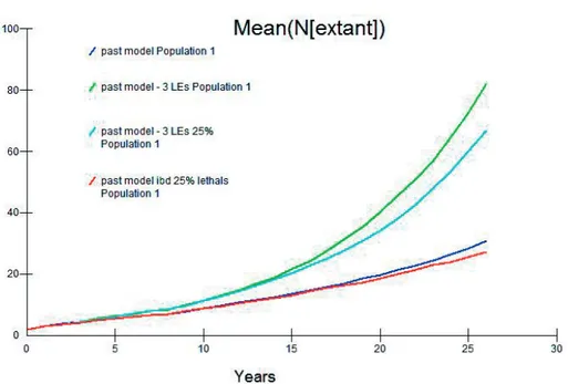
I also tested the influence of different inbreeding values on the model out-comes. While the number of Lethal Equivalents has been estimated at 6.04 (Liberg et al. 2005), the percentage of those due to lethal recessives is not known and Bensch et al. (2006) showed that in any case successful pairs have higher heterozygosity than would be predicted by chance for each level of inbreeding tested. I therefore examined the effects of changing inbreeding parameters, testing zero inbreeding, 3 Lethal Equivalent genes (the number of recessive lethal alleles in the genome; LEs), 6 Lethal Equivalents and the per-centage of inbreeding depression affecting survival due to lethal recessives (LRs; 50%, the standard model in VORTEX and 25%). Figure 2 shows the projected population sizes of the population assuming four configurations of inbreeding. The most optimistic model predicted a mean population size of 82 individuals at 2008 – this assumed 3 LEs and 50% LRs.

Figure 3 shows the change in inbreeding coefficient in the same

simula-tions, and indicates that, as expected, inbreeding accumulates more rapidly where the negative effects of inbreeding depression is least severe. However, interestingly the values were of the same order as those indicated by Åkesson et al. in the workshop in April 2013 and show a response to the first immigra-tion event. However, even under the least severe inbreeding model, the pro-jected population size at 2008 was only 57% of the actual value, suggesting inbreeding parameters should be manipulated further.

(18)

Figure 2 – The infl uence of inbreeding on the simulated Swedish wolf population size from founda-tion until 2008 (25 years).

Figure 3 – The infl uence of inbreeding on the simulated Swedish wolf population inbreeding coef-fi cient from foundation until 2008.

Evaluation of the fi rst model: analysis of the past population shows that the

Swedish wolf is a population that, given the parameters used here, might have been expected to go extinct. The fact that it did not could either be a result of chance or to a factor in its population dynamics that was not captured in the model. Of particular interest is the balance between inbreeding cost, fecundity and inter-birth interval. At the mid-term review, G. Chapron has

(19)

surmised that there is no reason why Swedish wolves should not be breeding each year. The implied deterministic lambda values, however, imply that it is unlikely that this is the case, and more likely favour the 29% female breeding value proposed in Nilsson (2004). I used a stable age distribution for the mod-eling, and an arbitrary population size, to enable the general attributes of the model to be discerned. There seemed to be general agreement around the 4–5 cubs per litter value, and the model was not very sensitive to this parameter, although a realistic standard deviation value needs to be applied. The inbreed-ing values are perhaps of more interest, and have a profound impact on the model, which is not surprising given its demographic history.

(20)

Model Refinement

Revised basic model

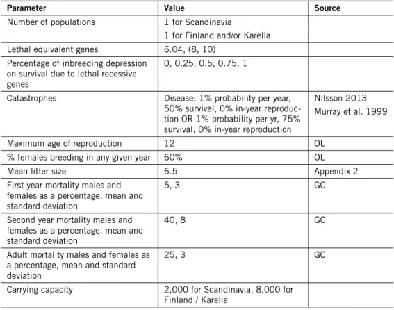
Following discussions at the mid-term review meeting (Appendix 1), a number of adjustments were made to the basic life history parameters used in the model, to reflect the best estimates available for the Swedish wolf population (Table 3).

Table 3 – Modified model parameters . OL = Olof Liberg, pers. comm., GC = Guillaume Chapron, pers. comm.

Parameter Value Source

Number of populations 1 for Scandinavia

1 for Finland and/or Karelia Lethal equivalent genes 6.04, (8, 10)

Percentage of inbreeding depression on survival due to lethal recessive genes

0, 0.25, 0.5, 0.75, 1

Catastrophes Disease: 1% probability per year,

50% survival, 0% in-year reproduc-tion OR 1% probability per yr, 75% survival, 0% in-year reproduction

Nilsson 2013 Murray et al. 1999

Maximum age of reproduction 12 OL

% females breeding in any given year 60% OL

Mean litter size 6.5 Appendix 2

First year mortality males and females as a percentage, mean and standard deviation

5, 3 GC

Second year mortality males and females as a percentage, mean and standard deviation

40, 8 GC

Adult mortality males and females as a percentage, mean and standard deviation

25, 3 GC

Carrying capacity 2,000 for Scandinavia, 8,000 for Finland / Karelia

Structured sensitivity testing was carried out to re-evaluate the population size, extinction probability and genetic diversity trajectories and their standard devia-tions for the Scandinavian population alone (analysed for consistency between 1983 and 2008), without the inclusion of catastrophes in the first instance. Two inbreeding parameters were first analysed independently, since this is known to be a major issue for this population (Ellegren 1999) and inbreeding is poorly incorporated into many population viability assessments (Frankham et al. 2013). First the percentage of genetic load attributable to recessive lethal genes was examined. This was because some discussion occurred at the mid-term review on the likelihood that genetic load could have been purged (removed by selec-tion) during the history of the Scandinavian wolf population. As expected, when the percentage load due to lethal equivalents was high, the population recovered more rapidly due to the effects of purging (removal of genetic load due to the death of homozygous individuals).

(21)

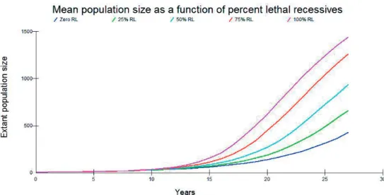
Recent research (e.g. Kennedy et al. 2014) has, however, questioned the role that purging plays in natural populations, especially when inbreeding levels have accumulated rapidly, as in the Scandinavian wolf. This is thought to be because inbreeding depression for many traits could involve many genes of weak deleterious effect. For the simulations carried out here, increasing the proportion of lethal recessive genes involved in genetic load had a predict-able and positive consequence for mean population growth (Figure 4). Using a percentage of recessive lethal values of 75 and 100, produced unrealistic population growth rates (standard deviations did not overlap with observed value of approximately 140 individuals at 2008), I confi ned further analysis to Recessive Lethal percentages of 50 and lower.’

Figure 4. The effects of purging of genetic load on the Swedish wolf population simulated from 1983 to 2008 (25 years) on extant population size (means of 1,000 simulations are shown). RL = recessive lethals.

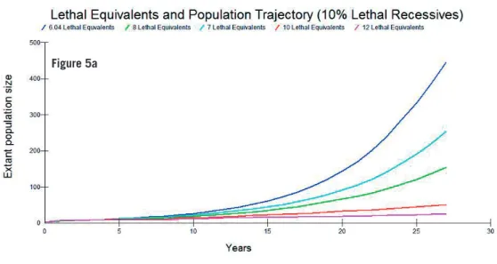
Next, the number of Lethal Equivalent genes (estimate 6.04; Liberg et al. 2005) was tested to explore higher values to account 1) for additional mortal-ity during period between December and the following May in the fi rst year of life when additional mortality may occur but which cannot be censused in the fi eld, and 2) inbreeding depression due to the lower probability of pairing that has been seen for inbred adults (Åkesson, pers. comm.). The number of lethal equivalent genes was set at 6.04, 7, 8, 10 and 12 to cover realistic values seen from other vertebrate species (O’Grady 2006). These were covaried with 0, 10%, 25% and 50% of genetic load attributed to lethal recessive alleles.

Figure 5 shows the results for 10%, 25% and 50% Lethal Recessives.

Although the standard deviations among some of the simulations over-lapped (not shown), the parameters best fi tting the observed population data at 2008 were 8 Lethal Equivalents for up to 50% Lethal Recessives; this number of equivalents is similar to the more recent estimate by Sand et al. (2014; their Fig. 15). I therefore chose to model these parameter combinations in further analysis.

(22)

Figure 5. Lethal equivalents and their effect on population trajectory for a) 10%, b) 25% and c) 50% Lethal Recessives (means of 1,000 simulations are shown).

Figure 5a

Figure 5b

(23)

The mean stochastic intrinsic growth rate estimates for these models varied between 0.107 and 0.153, all of which are below the recently estimated value of 0.181 (Chapron et al. 2012, estimated without inbreeding depres-sion modeling, although some of my standard deviations overlapped with that value), however the model estimates comprised the entire 25 year period between 1983 and 2008. A value of 10% recessive lethal genes has been pre-viously observed by Liebl et al. (2006), albeit for synaptogenesis mutants in Drosophila melanogaster, however such estimates are in general very difficult to find in the literature. O’Grady et al. (2013) found an average overall effect of 8.4 diploid lethal equivalent genes for survival to sexual maturity in a meta-analysis of vertebrate data.

To further evaluate the percentage of lethal recessives, the model was extended to 2014, thereby including a further immigration event in 2008, when two males immigrated into the population (Laikre et al. 2013). For this model, the percent lethal recessives was further refined to 10, 25, 30, 40 and 50. Table 4 summarises the most relevant results from these models. It should be noted that a limitation of the Vortex software is that deterministic immi-gration events are modeled by Supplementation. This option does not permit variation in the number of individuals entering the population between sup-plementation events. Therefore in this instance only the addition of a single adult male in 2008 (in addition to the individual in 1991) could be mod-elled. An alternative analysis involving the supplementation of two adult male individuals into the population was included, but this produced very similar results (not shown) to those presented below.

Table 4. Model parameters from Lethal Recessive analysis using eight lethal equivalents and five scenarios with different percentages of lethal recessives. Stoc-r : observed intrinsic growth rate, SD(r): standard deviation among simulation replicates, PE: probability of extinction for each model, N-extant: mean size of the surviving populations at the end of the simulation time-point, SD(Next): standard deviation, GeneDiv: recorded mean gene diversity of the population by the end of simulations, AllelN: number of extant alleles in the loci modeled, Mean F: average value of the population inbreeding coefficient (F) by the end of simulations.

Scenario stoc-r SD(r) PE N-extant SD(Next) GeneDiv AllelN Mean F

LR 10 0.114 0.422 0.618 233.62 357.59 0.6905 5.62 0.265

LR 25 0.13 0.414 0.59 358.92 496.38 0.692 5.79 0.284

LR 30 0.136 0.412 0.603 425.97 533.03 0.6745 5.82 0.295

LR 40 0.146 0.406 0.582 574.68 687.84 0.6844 5.84 0.273

LR 50 0.152 0.415 0.606 688.12 730.9 0.6684 5.8 0.309

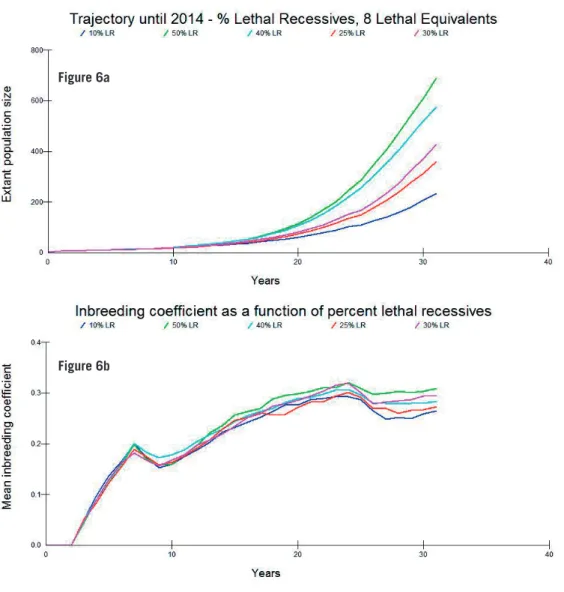
Figures 6a and b show the trajectories in population size and inbreeding

coefficient to 2014 under the same assumptions. The closest model to cur-rent observed estimates for population size assumes eight lethal equivalents and 30% lethal recessives. All models produced realistic results given the values that have been estimated from pedigrees. Mean inbreeding for litters of breeding wolf pairs in 2013 was approximately 0.25 (Åkesson, pers. comm.) whereas for the model, values for ranged between 0.265 and 0.309 – however

(24)

this value is a mean across all surviving individuals and average inbreeding of litters are lower than expected from the potential parents since immigrant off-spring have shown a higher pairing success (Åkesson, pers. comm.). Therefore the model chosen for further analysis was the one that most closely follows the current population trajectory, with a number of lethal equivalents of 8 and

percentage lethal recessives of 30.

Figure 6. Population size (a), and inbreeding trajectory (b) as a function of lethal recessive per-centages (means of 1,000 simulations are shown).

Catastrophes

With the basic parameters established, a model was constructed to examine population growth parameters in the absence of immigration for the coming 100 years (approximately 20 wolf generations) including and excluding catas-trophes (here modeled as disease outbreaks), following Nilsson (2013) and Murray et al. (1999). Nilsson (2013) modeled one severe disease epizootic per 100 years with 50% survival and 100% loss of reproduction for the year

Figure 6a

(25)

of event, while Murray estimated that population size changed by 25.2 ± 7.8 (SE)% for Canis lupus. Two models were therefore run, with the first follow-ing the Nilsson model and the second modelfollow-ing 75% survival. A comparison of model outcomes in terms of population trajectory and inbreeding coeffi-cient is shown in Figure 7a and b below. As can be seen, catastrophes had very little impact on the final size of surviving populations, which reached carrying capacity at Year 75 and where inbreeding coefficient remained at between 0.3 and 0.4 for the forecasting period. I therefore retained the catastrophe model described by Nilsson (2013) as the most conservative option.

Figure 7. Forward modeling of different catastrophe scenarios, a) population size and b) inbreeding coefficient (means of 1,000 simulations are shown).

Figure 7a

(26)

Forward modeling without gene

frequencies

Modeling immigration to the Scandinavian

population

The current Scandinavian population has a size of approximately 420 individ-uals with an inbreeding coefficient between 0.25 and 0.30. However, the ques-tion posed by SEPA is how strong is the effect of modest numbers of effective immigrants at population sizes of 170 (the lower bound of the Swedish Parliament’s Favourable Reference Population or FRP definition) through to greater than 417 (SEPA’s genetic minimum viable population size or MVP as a FRP) and within these value ranges, how many reproducing immigrants per generation will prevent significant inbreeding or loss of variation?

A structured analysis was therefore next carried out constraining the Swedish wolf population to 170, 270 (the Swedish Parliament’s upper bound FRP), 370, 420 (SEPA’s lower bound MVP is 417), 470 and 570. This was simulated as a managed translocation via regular and directed supplemen-tation of 1, 2, 3, 4 and 5 migrants per generation (defined here as 5 years). Where possible even numbers of both sexes were added. This model did not include gene frequencies, and assumed individuals at the start of the modeling were unrelated. The questions in italics were specifically addressed with this modeling.

How strong is the effect of modest numbers of effective immigrants at popula-tion sizes of 200–300? How many wolves per generapopula-tion will prevent signifi-cant inbreeding or loss of variation?

Changes in genetic diversity were estimated using gene diversity, inbreeding coefficient and allelic diversity. Figure 8 below shows the change in inbreed-ing coefficient predicted for population sizes 170, 270 (FRP bounds) and 370 under one and two immigrants per generation. The strongest effect could be seen in population size, since the two simulations featuring populations sized 370 showed the only below 10% increase in mean inbreeding coefficient (δF = 0.0894 for one immigrant per generation and 0.0824 for two immi-grants). This suggested that under modest immigration rates, population size (genetic drift) plays an important role in the maintenance of genetic diver-sity. The final values over 100 years for all three parameters are presented in

Table 5.

Further, if an aim is to conserve > 90% of gene diversity over 20 genera-tions (or even 40 generagenera-tions if a 200 year criterion is used; Soulé et al. 1986) with modest immigration rates (sometimes cited as a minimum target for short-term maintenance of genetic diversity in small populations), these results indicated that a population size of 370 individuals would be minimally needed (Table 5). While the effects of maintaining allelic diversity in natural

(27)

popula-tions have only been demonstrated for a few cases, it is worth noting that while allelic diversity inevitable declines steeply in populations undergoing genetic drift, the highest number of alleles are also maintained in larger population sizes (exceeding 20 only in populations of 370 individuals).

Figure 8. Inbreeding as a function of modest immigration at population sizes of 170, 270 and 370 (means of 1,000 simulations are shown).

Table 5. The effect of modest numbers of immigrants per generation on key genetic parameters after 100 years.

Proportion of gene diversity retained

Increase in mean

inbreeding coeffi cient Allelic variation

170 1 imm. per gen 0.8346 0.1541 12.95 270 1 imm. per gen 0.8778 0.115 16.95 370 1 imm. per gen 0.9041 0.0894 20.91 170 2 imm. per gen 0.86 0.1281 16.27 270 2 imm. per gen 0.8888 0.1037 19.84 370 2 imm. per gen 0.911 0.0824 24.02

In 2012, SEPA proposed a genetic MVP as a minimum value for FRP for the Scandinavian wolves at > 417 combined with effective immigration of > 3.5 reproducing wolves per generation. Does modeling confi rm the result of this assessment?

To address this question the same parameters were assessed by comparing the effects of higher immigration rates (3 and 4 per generation) across a range of population sizes from 170 to 570 (Table 6). In particular the proportion of genetic diversity retained at a population size of 420 (SEPA’s MVP) was com-pared to realistic and policy relevant values above and below that number. SEPA’s MVP value of 420 individuals was predicted to retain greater than 92% of current gene diversity over 100 years while constraining an increase in inbreed-ing coeffi cient to approximately 7% over 20 wolf generations, and retaininbreed-ing approximately 50% more allelic diversity than the 170 lower limit FRP value.

(28)

Table 6. The effect of larger numbers of immigrants (3, 4) per generation on key genetic parameters after 100 years as a function of population size. SEPA’s MVP value is shown in bold.

Proportion of gene

diversity retained Increase in mean inbreeding coefficient Allelic variation

170 3 imm. per gen 0.8753 0.1127 18.78

270 3 imm. per gen 0.898 0.095 23.05

370 3 imm. per gen 0.9153 0.0793 26.95

420 3 imm. per gen 0.9234 0.0705 29.13

470 3 imm. per gen 0.9289 0.0663 30.99

570 3 imm. per gen 0.9382 0.0574 35.03

170 4 imm. per gen 0.8873 0.1005 21.34

270 4 imm. per gen 0.9054 0.0867 25.66

370 4 imm. per gen 0.9203 0.0734 29.66

420 4 imm. per gen 0.9266 0.0671 31.48

470 4 imm. per gen 0.9308 0.0636 33.57

570 4 imm. per gen 0.9407 0.0554 37.73

It is the case that larger population sizes, as expected, retain ever-greater levels of diversity (as much as 94% of gene diversity and constraining inbreeding to a 5.5% increase over 100 years for a population of 570 and four migrants every five years).

Under relatively high rates of immigration (4 per generation), the upper bound FRP size proposed by the Swedish parliament is predicted to retain slightly in excess of 90% initial gene diversity and increase its mean inbreeding coefficient by 8.7%. Retention of 90% of initial heterozygosity over 200 years has been cited as a minimal requirement for maintenance of genetic diversity in captive breeding programs (Soulé et al. 1986) – it is worth noting that a popula-tion size of 270 was not predicted to reach this threshold for one, two or three migrants per generation, but was predicted to be achieved with four effective migrants and higher. The likelihood that this level of effective immigration can be achieved on the ground might therefore be the deciding factor on the popula-tion size that should be retained.

The definition of “sufficient genetic variation” for short-term population via-bility is a matter of considerable scientific debate. The Scandinavian wolf popu-lation descends from five individuals and Frankham et al. (2013) argue that an effective population size of greater than 100 is required to limit loss in total fit-ness to 10%. The modeling presented here shows that a balance will need to be struck between population size and immigration to reach this goal. It seems from these modeling results that a loss of gene diversity and an increase in inbreeding coefficient of within 10% to be achievable in larger population sizes (370 and greater) with as little as one effective migrant per generation.

The modeling methods used here were by no means exhaustive and would be improved in a number of ways. Importantly, the second modeling objective identified at the mid-term review, to simultaneously model the Scandinavian and Finnish/ Karelian population has been attempted but did not perform reliably due to difficulties in implementing a complex historical scenario with forward casting in VORTEX (not reported here), uncertainties on the demographic history of the Karelian population and its demographic relationship with the Finnish

(29)

popula-Two further customised models

Reviews of the report describing the Forward Modeling Without Gene

Frequencies were received from five independent reviewers and one group,

plus SEPA. The reviews included suggestions for modifications and clarifica-tions of in final report including reporting of the modeling results and tex-tural changes, but notably included suggestions for additional modeling and requests to more specifically address the legal issues and questions in SEPA’s decision letter. A summary description of consensus points from the reviews with specific issues highlighted of importance for the revised modeling is reported in Appendix 2.

Basic parameters

Basic values for the models described in this section were established at the mid-term review and are summarized in Table 1. There was broad consen-sus among the reviewers that the biological parameters used adequately represented current knowledge of the Swedish wolf population. However, a number of changes were suggested. The first change concerned altering the mating system specified from ‘Monogamy’ (monogamy in any given year but a random probability of mating with the same individual in following years) to ‘Long-term Monogamy’ (the same individuals breed together annually until one dies). This change did not affect the outcome of a subset of Final Report models that were tested (see Supplementary Table 1): results obtained were very similar to those obtained using short-term monogamy. Long-term monogamy was retained for further modeling to better reflect the breeding biology of the species. These parameters were also used to examine for any (unexpected) systematic differences in modeling outcomes for Vortex v9.99 versus Vortex v10 because further modeling utilized functionality for handling additional genetic data that has been improved in Vortex v10 by RC Lacy. As expected, the results were almost identical, recovering the same or very similar values for all models tested, as could be expected under stochastic simulation (Supplementary Table 2).

Model Structure

The most important and fundamental changes in the modeling approach, identified by several of the reviewers (and highlighted in the Final Report) was the need to include more pedigree information, and to more accurately reflect genetic differentiation between the Scandinavian wolf population and the likely source populations for future immigration (Finland / Karelia). However, computational capacity and software functionality constraints in Vortex cur-rently prevent these two issues being modeled simultaneously. Specifically, 1) it is not possible to model multiple populations with different demographic

(30)

profiles (described using a pedigree file), even if such data are available (which they are not for Finland and Karelia) and 2) because inbreeding depression, which is computationally intensive to model, must be applied to all popula-tions, it was not possible using the computational capacity available to model three populations simultaneously – only two could be included.

To address the first issue, additional modeling was carried out using ped-igree data kindly supplied by Dr Mikael Åkesson (Grimsö Wildlife Field Station, Swedish University of Agricultural Sciences) for a subset (320) of living animals from the Swedish wolf population of 2012. These data, which included individual relationships and inbreeding coefficients, were linked to Vortex to test the impact of different levels of immigration, which could only be modeled using Vortex’s Supplementation routine due to functionality con-straints when pedigree files are used, and using different carrying capaci-ties for the Scandinavian population (200–700), specified by SEPA following review of the report on the Forward Modeling Without Gene Frequencies. The disadvantage with using the supplementation option in this context (as pointed out in reviews of the final report) is that the alleles carried by supple-mented individuals are unique, which in this case is likely to overestimate the genetic benefit of immigration because in reality the allele frequencies of natu-ral immigrants would be expected to be correlated with the Scandinavian pop-ulation, reflecting the genetic similarity of subpopulations within the northern European metapopulation.

To address the above issue, additional modeling was carried out for the Scandinavian population and a notional second population (with size 1,000 and carrying capacity 2,000 to constrain computational load) that genetically resembled the Finland/Karelian population. Allele frequencies for ten micro-satellite genetic profiling markers (kindly supplied by Dr Mikael Åkesson) were utilized for the Scandinavia and Finland/Karelia populations. Here, Scandinavian and Finnish allele frequencies were used with the Vortex genetic management utility, and combined with bidirectional and unidirectional dis-persal, and different carrying capacities in Scandinavia for a subset of simula-tions (see below).

In both cases, a key question is what constitutes ‘genetically effective’ immi-gration, as opposed to demographic immiimmi-gration, since equating demographic immigration to gene-flow assumes that all immigrants will remain, survive and breed, which is not the case, since 12 individuals immigrated into Scandinavia between 2002 and 2009 (approx. 1.5 per year; SOU 2012:22) and because between 2008 and 2012, four immigration events occurred and only two of those are known to have been genetically effective (0.4 genetically effective migrants per year, approximately two individuals per generation). Both these ‘pedigree + supplementation’ and ‘allele frequencies + dispersal’ models used a range of supplementation/ dispersal values to cover most foreseeable scenarios, ranging from zero to two effective migrants per year (see below). All modeling reported hereon was carried out using Vortex v10. Using replicated subsets of the simulations, results converged before a total of 1,000 simulation replicates

(31)

The pedigree + supplementation model

To establish that using the pedigree data yielded more realistic estimates of genetic diversity and inbreeding in the current Scandinavian population, simulations were carried out using these data to examine the magnitude and trajectory of inbreeding and heterozygosity in the in the absence of immi-gration with a carrying capacity set at a notional 700 wolves (Figure 9a, b). Simulations were carried out over 50 years (approximately 10 wolf genera-tions). The mean starting inbreeding coeffi cient was 0.267 ± 0.041 (SD) and as can be seen in Figure 9a, initially the inbreeding coeffi cient underwent a decline before gradually increasing to a fi nal mean value of 0.348 ± 0.078 (SD). These values and (initial) trajectory are similar to the empirical values that have been reported by Åkesson et al. (pers. comm.). Figure 9b shows the trajectory of gene diversity (heterozygosity) in the absence of immigration and the values estimated from the pedigree genetic data agree closely with cur-rent molecular estimates (Åkesson et al.). The fi nal (year 50) value of 0.642 ± 0.075 (SD) implies a mean decline of 0.082 from an initial value of 0.724. However, it should be pointed out that for both parameters, standard devia-tions overlap substantially for the duration of the model. The mean fi nal pop-ulation size was 550 ± 237 (carrying capacity 700).

Figure 9a. Inbreeding coeffi cient in the Scandinavian wolf population starting from 2012 pedigree values in the absence of immigration. Means and standard deviations of 1,000 simulations are presented.

Immigration was then simulated with the pedigreed dataset, using supplemen-tation over a 50-year period, with different frequencies to represent a spread of possible effective immigration rates, with a notional carrying capacity of 700 wolves. Figure 10a shows the effect of different immigration rates, rang-ing from one female per 12 years (2–3 wolf generations) through to four effective immigrants per three years. In contrast to the results reported using

(32)

the idealized population simulated in the Forward Modeling Without Gene Frequencies analysis, as few as one female per three years produced a substan-tial decrease in the mean inbreeding coeffi cient compared to its starting value (fi nal value 0.214 ± 0.037 SD) and even immigration of one female per six years (approximately one migrant per generation) resulted in a slight decrease in mean inbreeding coeffi cient, using a carrying capacity of 700, although again standard deviations overlap considerably (0.250 ± 0.037).

Figure 9b. Gene diversity in the Scandinavian wolf population starting from 2012 in the absence of immigration. Means and SDs of 1,000 simulations are presented.

Figure 10a. Inbreeding coeffi cient in the Scandinavian wolf population starting from 2012 pedi-gree values using a carrying capacity of 700 with population supplementation. Means of 1,000 simulations are presented.

(33)

Figure 10b shows the trajectory in gene diversity for the same set of

simula-tions. The supplementation of one female every 6 years resulted in a slight increase in mean gene diversity to 0.743 ± 0.045 SD. While populations sup-plemented every 12 and six years did not achieve carrying capacity, although SDs overlapped (628 ± 170 and 662 ± 116, respectively), all other simulations achieved mean fi nal population sizes very close to 700.

Figure 10b. Gene diversity in the Scandinavian wolf population starting from 2012 pedigree values using a carrying capacity of 700 with population supplementation. Means of 1,000 simulations are presented.

A subset of the supplementation scenarios were then subjected to variation in carrying capacity (k = 200, 300, 400, 450, 500, 600, 700) to assess whether a systematic effect of carrying capacity and hence (in most cases) population size could be detected under similar ranges of supplementation, as had been found in the previous modelling. In these simulations, the effect of popula-tion size was very moderate compared to the effect of supplementapopula-tion rate.

Figure 11 shows the change in inbreeding coeffi cient as a function of

sup-plementation frequency (no supsup-plementation, one female per 12 years, one female per six years and one female per three years), with the effect of carry-ing capacity explored only in the latter two categories. Surpriscarry-ingly, no effect on mean inbreeding could be inferred for any given level of supplementation (for a more detailed graph, see Supplementary Figure 1) with the smallest car-rying capacity (k = 200) showing slightly larger increases in mean inbreeding coeffi cient, although this is not evident in all supplementation combinations (Supplementary Table 3), although mean fi nal coeffi cients declined as a func-tion of supplementafunc-tion rate (from 0.318 to 0.147; Supplementary Table 3).

(34)

Table 7 shows summary results for key scenarios in fi nal population

param-eters for supplementation rates as a function of carrying capacity (full results can be found in Supplementary Table 3). Population sizes reported are means across years as opposed to mean fi nal values. Mean fi nal inbreeding coef-fi cients decreased from present-day values in all cases and mean coef-fi nal Gene Diversity values exceeded present day values in all cases, regardless of car-rying capacity. However, while the relative magnitude of these trajectories is informative, especially among supplementation scenario groups, their absolute value is questionable due to the unrealistic assumption of the supplementation regime in Vortex, which is why the ‘allele frequencies + dispersal’ model was also explored (below). Stochastic-r (the stochastic population growth rate) is calculated using the simulated birth and death rates in the model, whereas the deterministic growth rate simply uses the demographic parameters in the model as fi xed. Stochastic-r values are almost always smaller than determin-istic r -values (Lacy et al. 2014), and in Vortex this is because multiplicative effects of population fl uctuations in growth and survival, because determin-istic growth parameters assume a starting stable age distribution, and most importantly because of density dependent effects and especially inbreeding at small population sizes. In the case of the pedigree + supplementation model, it is likely that these inbreeding effects are the predominant cause of the dis-parity between stochastic and deterministic growth. Identifying the precise demographic factors underpinning lower growth rates in inbred populations is, however, highly challenging (Keller et al. 2012).

Figure 11. Inbreeding coeffi cient in the Scandinavian wolf population starting from 2012 pedigree values using carrying capacities of 200–700 with population supplementation ranging from zero to one female per three years. Means of 1,000 simulations are presented.

(35)

Table 7. Key model outcomes at 50 years for the Scandinavian wolf population with 2012 pe-digree values, carrying capacities of 200–700 with population supplementation. Supplementary Table 3 presents the full range of results.

Scenario Stochastic r (growth rate) SD (r) Mean Population size SD Population size Gene diversity SD (GD) Percentage of initial Gene Diversity retained Inbreeding coefficient One female/ 3 years k200 0.139 0.23 192.86 23.14 0.769 0.04 106.2 0.223 One female/ 3 years k450 0.141 0.232 435.94 51.66 0.78 0.038 107.7 0.22 One female/ 3 years k700 0.142 0.23 679.06 85.92 0.782 0.037 108.0 0.221 One pair/ 3 years k200 0.171 0.241 196.01 19.31 0.818 0.032 112.9 0.184 One pair/ 3 years k450 0.176 0.235 438.02 49.65 0.823 0.031 113.7 0.186 One pair/ 3 years k700 0.175 0.233 684.94 71.11 0.823 0.033 113.7 0.186 Two females and two males/ 3 years k200

0.214 0.245 195.63 20.54 0.863 0.023 119.2 0.143

Two females and two males/ 3 years k450

0.215 0.238 491.36 46.32 0.867 0.023 119.8 0.145

Two females and two males/ 3 years k700

0.216 0.236 689.84 55.48 0.865 0.024 119.5 0.147

The allele frequencies + dispersal model

To model the potential genetic dividend of immigration into the Scandinavian wolf population using genetic data, microsatellite marker (DNA profile) allele frequencies were used to describe the genetic diversity and differentiation within and among the Scandinavian and Finland/Karelia populations. DNA profile frequencies were provided courtesy of Dr Mikael Åkesson, and these were used with the Vortex genetics module as follows. Ten profiling markers (the maximum number permissible in Vortex) were selected (20, 225, 2001, 2010, 2088, 2168, AHT101, vWF, PEZ03, AHT126) and the allele frequen-cies for each marker for live individuals from 2012 were used to specify the starting genetic allele frequencies for the model. However, computational capacity prevented all three populations and all ten loci being modeled simul-taneously, probably because inbreeding depression can only be applied to all populations simultaneously in the model. I therefore chose to use the Finland population allele frequencies for the second population, as Finland is most proximate and immigrants are most likely to come from this source (see Seddon et al. 2006; Kojola et al. 2009). However, to acknowledge the ongoing gene-flow and connectedness between the populations in Finland and Karelia, I used a notional starting population size of 1,000 individuals with a carrying capacity of 2,000. Allele frequencies for the first five markers were selected although parallel simulations using the second five markers were carried out as a control for a small number of scenarios and the results were similar (data

(36)

First, and to enable a direct comparison of the genetic parameters computed using Vortex for the Scandinavian population in isolation with the ‘pedigree +

supplementation’ model, simulations were conducted using starting allele

fre-quencies for the Scandinavian population alone. The initial (2012) population size was specifi ed as 320 individuals (for direct comparison with the pedigree model) with a stable age distribution and simulations were conducted over 50 years (approximately 10 generations) with a notional carrying capacity of 700. Figure 12a shows the trajectory in inbreeding coeffi cient and Figure 12b shows the trajectory for gene diversity. The mean starting inbreeding coeffi -cient was 0.277 ± 0.007 and the mean gene diversity was 0.722 ± 0.002.

Figure 12a. Inbreeding trajectory in the dispersal model without immigration (carrying capacity 700). Means and standard deviations of 1,000 simulations are presented.

Figure 12b. Gene diversity trajectory in the dispersal model without immigration (carrying capacity 700). Means and standard deviations of 1,000 simulations are presented.

(37)

These values, while not identical to those estimated from the pedigree data, are within a single standard deviation and are almost identical for gene diver-sity. The estimate of mean inbreeding coeffi cient in this model is calculated using the homozygosity estimated from the user-defi ned starting allele fre-quencies (R.C. Lacy, pers. comm.). Note, mean population size across all years of the simulation was 695.41 ± 18.37. Although the mean fi nal inbreeding coeffi cient was lower for the dispersal model, the mean fi nal values and their distribution overlapped almost entirely between suggesting that although the source of genetic data in the two models was different, the model assumptions produced convergent estimates of genetic diversity.

Next, immigration was simulated for a Scandinavian population using the same carrying capacity (700 individuals) with immigration rates varying from one immigrant per twelve years to six immigrants per three years (see below). Mean fi nal inbreeding coeffi cients were surprisingly similar across simulations, ranging from 0.271 ± 0.019 (SD) for six immigrants per three years to 0.291 ± 0.015 (SD) for one immigrant per twelve years and standard deviations overlapped. Figure 13 shows that for both six and three effective migrants per three years an improvement or parity in mean inbreeding coeffi cient, respec-tively, was produced whereas two effective immigrants per three years or less resulted in an increase. The magnitudes of these effects (also evident for gene diversity, not shown) are much smaller for the dispersal model than for the pedigree-based model, albeit at a higher carrying capacity (and population size), reinforcing the importance of the assumptions of genetic similarity of immigrants on genetic diversity indices.

Figure 13. Inbreeding trajectory in the dispersal model with immigration (carrying capacity 700). Means and standard errors of 1,000 simulations are presented.

(38)

Two additional carrying capacities were applied, using the immigration rates identifi ed in the k = 700 simulation as not resulting in an increase in inbreed-ing coeffi cient, in order to establish whether carryinbreed-ing capacity per se (hence population size, since all simulations gave mean population sizes within one standard deviation of the carry capacity, not shown) constrained changes in inbreeding and gene diversity and to provide two direct points of comparison (k = 500 and k = 300) with the pedigree + supplementation model. Figure 14 shows the trajectory of inbreeding coeffi cient in these simulations and shows that six effective immigrants per three years resulted in a decrease in mean inbreeding coeffi cient over 50 years with the largest magnitude of change (> 0.01) for carrying capacities of 300 and 500 (0.267 ± 0.010 and 0.268 ± 0.007, respectively). The mean fi nal gene diversities for these simulations also showed the largest increases (to 0.728 ± 0.015 SD and 0.729 ± 0.16, respec-tively). Table 8 summarises the outcome for these simulations. Key scenarios and full outcomes are reported in Supplementary Table 4. In sum, under the assumptions of the allele frequencies + dispersal model, the genetic dividend of the highest immigration rates (six effective immigrants per three years) is most strongly felt at lower carrying capacities/population sizes, although these effects remain subtle and standard deviations overlap.

Figure 14. Inbreeding coeffi cient trajectory for three and six immigrants per three years as a func-tion of carrying capacity (700, 500, 300) for Scandinavia. Means and SE of 1,000 simulafunc-tions are presented.