Department of Economics
Working Paper 2011:15
Job Polarization and Task-Biased
Technological Change: Sweden, 1975–2005
Adrian Adermon and Magnus Gustavsson
Department of Economics Working paper 2011:15
Uppsala University September 2011
P.O. Box 513 ISSN 1653-6975
SE-751 20 Uppsala Sweden
Fax: +46 18 471 14 78
Job Polarization and Task-Biased Technological Change: Sweden, 1975–2005
Adrian Adermon and Magnus GustavssonPapers in the Working Paper Series are published on internet in PDF formats.
Job Polarization and Task-Biased Technological Change:
Sweden, 1975–2005*
September 21, 2011
Adrian Adermon♣ and Magnus Gustavsson♦
Abstract
This paper investigates the connection between the Swedish wage profile of net job creation and Autor, Levy, and Murnane’s (2003) proposed substitutability between routine tasks and technology. We first show that between 1975 and 2005, Sweden exhibited a pattern of job polarization with expansions of the highest and lowest paid jobs compared to middle-wage jobs. We then use cross-sectional and longitudinal analyses of job-specific employment to map out the importance of routine versus nonroutine tasks for these changes. Results are consistent with substitutability between routine tasks and technology as an important explanation for the observed job polarization during the 1990s and 2000s, but not during the 1970s and 1980s. In particular, the overrepresentation of routine tasks in middle-wage jobs can potentially explain 44 percent of the growth of low-wage jobs relative to middle-wage jobs after 1990 but largely lacks explanatory power in earlier years.
Keywords: Inequality; Job Mobility; Skill Demand; Skill-Biased Technological Change JEL Classifications: E24; J21; J23; J62; O33
* We are grateful to Per-Anders Edin, Maarten Goos, Nils Gottfries, Mikael Lindahl, Martin Nybom, and
seminar participants at Uppsala University, the 2010 UCLS workshop, and the 2011 National Conference of Swedish Economists for useful comments. We wish to thank Marteen Goos, Alan Manning, and Anna Salomons for providing some of the data used in this paper. Magnus Gustavsson acknowledges financial support from the Swedish Council for Working Life and Social Research.
♣ Uppsala University, Department of Economics and UCLS, Box 513, SE-751 20 Uppsala, Sweden;
Adrian.Adermon@nek.uu.se
♦ Uppsala University, Department of Economics and UCLS, Box 513, SE-751 20 Uppsala, Sweden;
1 1. Introduction
Technological progress is commonly believed to increase labor demand for more-skilled workers relative to less-skilled workers. Most notably, this notion of ‘skill-biased technological change’ (SBTC) has long been a workhorse in the literature on changes in wage dispersion and returns to skills (for overviews, see Katz and Autor, 1999; Acemoglu and Autor, 2011). However, SBTC also has implications for the composition of jobs in an economy. In the typical textbook model, technology-induced shifts in labor demand that push the returns to skills above its long-run equilibrium will make it increasingly attractive for individuals to acquire skills—along the lines of standard human capital theory—and thus also produce a continuous increases in the supply of skills (see e.g. Atkinson, 2008). Since there are increases in both the demand and supply of skills, ongoing SBTC is expected to yield a monotonic growth in the number of more-skilled to less-skilled jobs.
Recently, however, U.S. and U.K. studies have documented a rising share of not only the highest-paid jobs but also of the lowest-paid jobs (e.g. Goos and Manning, 2007; Autor, Katz, and Kearney, 2008; Autor and Dorn, 2010). Presumed that wages can be thought of as a single-index of worker skills, this pattern appears inconsistent with the implications of SBTC, where higher-paid jobs should simply increase relative to lower-paid jobs. Instead, as first demonstrated by Goos and Manning (2007), this pattern of ‘job polarization’—the disproportionate growth of both the lowest- and highest-paid jobs—is more consistent with Autor, Levy, and Murnane’s (2003) (ALM henceforth) proposed substitutability between routine tasks and technology and the notion of ‘task biased technological change’.
ALM make an important distinction between labor performing routine and nonroutine tasks and argue that the falling price of computer power should yield a drop in the relative demand for labor performing routine tasks (e.g. bookkeepers, repetitive production work). This follows from the observation that computer-driven technology can primarily replace human labor in routine tasks—tasks that can be expressed by rules or step-by-step procedures—but not (as yet) in nonroutine jobs. Goos and Manning (2007) in turn highlight that this fits well with job polarization since routine tasks are most common in middle-wage jobs. Top-paying jobs on the other hand consist of tasks that require nonroutine cognitive skills (e.g. engineers, economists) which should be complementary to computers, and the bottom of the wage distribution consists of jobs with a high degree of nonroutine manual tasks (cleaners, waiters, janitors) which should, according to ALM, be neither complements nor substitutes to computers. ALM’s hypothesis combined with the observed job polarization
2
thus implies a rise in the demand for low-wage workers relative to middle-wage workers and thereby—compared to traditional SBTC—offers a more nuanced view of how technology, and computers in particular, affects the demand for labor of different skills.
In light of these previous studies, the purpose of this paper is twofold. First, to thoroughly document the wage profile of net job creation in Sweden between 1975 and 2005, and second, to investigate if the observed job patterns are linked to the extent of routine versus nonroutine tasks across the job distribution along the lines predicted by ALM’s task biased technological change (TBTC henceforth) hypothesis. In doing so, we provide three new innovations to the empirical literature on job polarization. First, we use a bootstrap procedure to test if the observed pattern of net job creation is statistically significant. Tests of statistical significance are not carried out in previous studies, and our results show that such tests can substantially alter conclusions. Second, we invoke longitudinal data and study if individual mobility across routine and nonroutine jobs is along the lines expected from TBTC. Third, based on “back-of-the-envelope” calculations, we estimate the explanatory power of the distribution of routine and nonroutine tasks for the observed relationship between wages and net job creation.
Since most of the previous research on job polarization pertains to the U.S. and U.K., Sweden is also a particularly interesting country to study because in many regards it lies at the opposite end of the institutional spectrum. In particular, Sweden has one of the world’s most compressed wage structures, strong and influential unions, high levels of employment protection, and generous unemployment benefits combined with a well-developed welfare system (see e.g. Cahuc and Zylberberg, 2004; Björklund and Freeman, 2010). Several studies have suggested that this could yield a different pattern of net job creation. Acemoglu (2001) shows within a matching framework of the labor market that generous unemployment benefits and high minimum wages—as can be found in Sweden—induce incentives that should shift the composition of employment towards high-wage jobs. On the other hand, Acemoglu (2003) suggests a model in which union-imposed wage compression encourages the adoption of technologies that increase the productivity of less-skilled workers and thus induces positive effects on labor demand for these groups. Acemoglu and Autor (2011) also discuss the possibility that powerful unions could restrict or delay the substitution of machines for tasks performed by labor. Hence, even though Sweden certainly could access the same technology as the U.S. and U.K., the marked differences in institutional prerequisites need not imply job polarization in Sweden, even if TBTC should be true for the U.S. and U.K.. However, finding the same empirical relationships in Sweden as in the U.S. and U.K. would obviously
3
strengthen the TBTC hypothesis, suggesting that the incentive to replace routine manual tasks with technology could be strong enough to penetrate different institutional settings.
Previewing the main results, we find that net job creation in Sweden does indeed display a clear pattern of job polarization over the full period 1975–2005. Dividing the analysis into the two sub-periods 1975–1990 and 1990–2005 does however show much stronger evidence for polarization in the later period. Our investigation of the relationship between routine and nonroutine tasks across jobs and the observed changes in employment also speaks against TBTC as an important explanation for the overall pattern of job creation in Sweden during the 1970s and 1980s, but provides strong evidence for the hypothesis during the 1990s and 2000s. After 1990, there are significant declines of routine jobs and expansions of cognitive non-routine jobs both between and within industries. Using the longitudinal dimension of our data, we also find a clear pattern of job mobility away from routine jobs towards cognitive nonroutine jobs during the 1990s and 2000s. Finally, we use regression estimates to show that the distribution of routine versus nonroutine jobs, and thereby TBTC along the lines of ALM, can potentially explain 44 percent of the growth of low-wage jobs relative to middle-wage jobs after 1990 but largely lacks explanatory power for earlier years. Our mixed support for TBTC depending on the time period under study is broadly in line with the U.S. study of Autor, Katz, and Kearney (2008) who report evidence of job polarization for the 1990s but not the 1980s.
No previous study has made a formal statistical investigation of the connection between job tasks and the wage profile of employment creation in Sweden. In fact, most previous research, regardless of country, has primarily drawn conclusions based on visual inspections of distributions of routine and nonroutine tasks across the wage ranking of jobs. Important exceptions are Goos, Manning, and Salomons (2009, 2010) who rely on a regression framework to investigate the cross-sectional connection between tasks and employment changes in Western Europe. Our corresponding estimates corroborate their findings of a negative effect of routine tasks and a positive effect of cognitive nonroutine tasks on job-specific employment.
Some previous studies have, to some extent, aimed at documenting the wage-quality of net job creation in Sweden. Fernández-Macías and Hurley (2008) use the European Union Labour Force Survey (ELFS) and report a pattern of skill upgrading in Sweden since the mid 1990s. However, based on the same data source, Goos, Manning and Salomons (2009) instead report evidence of job polarization in Sweden over this period. A possible explanation for the
4
contradicting results is differences in data processing.2 Åberg (2004) uses Swedish data and
finds a pattern of skill upgrading between 1977 and 2001. His applied sample is however small—the sample we use is more than twenty times larger—and we believe this to be the main explanation for the difference between his and our results.
The rest of this paper proceeds as follows. Section 2 discusses the data and the empirical methodology. Section 3 presents the wage profile of net job creation between 1975 and 2005 and its connection to routine versus nonroutine tasks. The paper ends with concluding remarks.
2. Data and methodology
The primary data for this paper comes from the Swedish longitudinal micro-database LINDA. Beginning in 1968, for each year it contains a representative sample of 3.3 percent of the Swedish population (see Edin and Fredriksson, 1998, for details). We use data for three years: 1975, 1990, and 2005. Unlike for most other years, these three waves of LINDA contain detailed data on individuals’ occupations, labor income, and hours worked. It is also possible to translate occupational classifications across these three years; see the appendix for details.
LINDA is made up of different registers and surveys. For the years 1975 and 1990, we primarily use information collected from the Swedish Population and Housing Census (“Folk- och bostadsräkningen”, FoB). For the year 2005, we primarily use information collected by Statistics Sweden through individuals’ employers in the Linda Wage Survey. Individuals and employers are obligated by law to respond in their respective surveys. As a consequence, response rates are above 97 percent. An attractive feature of LINDA is its longitudinal dimension where, because of the link to registers and the very high response rates in the surveys, outflow occurs primarily because of death or migration from Sweden.
Our approach to investigate net job creation in high-, middle-, and low-wage jobs builds on a methodology first proposed by Joseph Stieglitz while in the Clinton administration and later refined and extended by Wright and Dwyer (2003) and Goos and Manning (2007). In a first step, we define a job as a particular occupation in a particular industry. We use three-digit SSYK coding for occupation and two-letter SNI 2002 coding for industry. This gives an
2 The aim of these two studies is to provide broad overviews of occupational changes in a large set of European
countries since the mid 1990s and this requires the data to be harmonized across countries. This harmonization differs across Fernández-Macías and Hurley (2008) and Goos, Manning and Salomons (2009). Their results for the rest of the investigated countries do also, to some extent, differ, with much stronger support for polarization across Europe in Goos, Manning and Salomons (2009).
5
industry/occupation matrix with 3,503 job cells. Individuals are placed in cells and weighted by their regular working time so that each cell contains the number of full time workers with a particular job. Since many cells are empty or have very few people in them, we are left with 1,377 jobs for our analysis. These jobs contain nearly all individuals. The appendix contains a detailed description of the data and our processing.
In the next step, we rank jobs according to their median wage in the first year, 1975, and group them into quintiles based on their median wage and cell size in that year. That is, we group jobs into the lowest paid 20 percent (quintile 1), the second lowest paid 20 percent, up to the top 20 percent based on their median wage and cell size in 1975. To study net job creation in different parts of the wage distribution for jobs between 1975 and 2005, we compute changes in the number of jobs—individuals in a particular occupation in a particular industry—in each of the 1975 quintiles. In other words, the numbers of individuals in 1975 that have jobs that are in the lowest paid quintile are compared to the number of individuals in the same jobs in 2005. This gives net job creation of the lowest paying jobs. For instance, assume that 50,000 individuals (in full-time equivalents) are employed in the jobs that in 1975 were classified into the lowest paid quintile whereas in 2005 the same jobs hold 100,000 individuals (in full-time equivalents); this means that there has been a net job creation of the lowest paid jobs by 50,000 units. The same is done for jobs in each of the 1975 quintiles.
For this empirical methodology to be valid the wage ranking of jobs must be stable over time; relatively low-wage jobs in 1975 should also be relatively low-wage jobs in 2005. Between 1975 and 2005, the rank correlation for all jobs in our analysis is above 0.8, and assigning jobs to quintiles based on wages and employment in 2005 instead of in 1975 does not change any main results in our analysis (available on request). We therefore argue that the wage ranking is indeed sufficiently stable for our purposes.
In the data, some jobs disappear while new ones pop up in later years. Most such jobs have very few individuals in them and the great majority is due to statistical changes in how occupations are classified over time. In our main analysis, we only include those jobs that are present in 1975.3
3 We have performed several sensitivity analyses related to this. First, we have assigned jobs into quintiles based
on their wage and employment in 2005 and then only included jobs that are present in 2005 (the opposite to our main approach). Second, we have only included jobs present in both 1975 and 2005. Third, we have as far as possible recoded (admittedly ad hoc) jobs that are new in 2005 into the 1975 classification. None of these approaches change our conclusions (results are available on request). In practice therefore, new and disappearing jobs do not seem to be a significant problem for our analysis.
6
We primarily focus on quintiles rather than, say, percentiles because of the significant changes in the statistical classifications of jobs over time; see the appendix. The measurement errors associated with these statistical reclassifications should be less of a problem within quintiles since the errors are likely to sum to zero, or at least more likely to sum to zero than within more fine grained divisions of the wage ranking. We do however rely on changes within percentiles in some parts of our analysis; the potential influence of measurement errors should be kept in mind when viewing these results.
To translate changes in our sample into aggregate changes for the whole of Sweden, we use information on aggregate employment from Statistics Sweden. For each year, we first convert aggregate employment into full-time equivalents based on the distribution of hours worked in our LINDA sample. The number of individuals in our year-specific samples is thereafter rescaled to equal the aggregate number of full-time jobs in the economy for the same year. These rescaled samples are then used to calculate aggregate employment changes across quintiles.
To investigate the connection between routine and nonroutine tasks and changes in employment—in light of the TBTC hypothesis—we use the three task measures developed and kindly provided to us by Goos, Manning, and Salomons (2009, 2010) of how intense occupations are in tasks labeled as abstract, routine and service. The three task measures are constructed from 96 variables in the December 2006 version of the US Occupational Information Network (O*NET) database through the use of principal component techniques. O*NET provides data on worker characteristics, worker requirements and general work activities for 812 U.S. occupations, information that in turn comes from job incumbents, occupational analysts and occupational experts. A detailed explanation on the development of these measures can be found in Goos, Manning, and Salomons (2010).
The link between computers and the three task measures are as follows. Routine tasks are intense in both cognitive and noncognitive routine skills and computers can perform these with relative ease, such as jobs that require the input of repetitive physical strength or motions, as well as jobs that require repetitive and non-complex cognitive skills. Abstract and
Service tasks are both in the nonroutine dimension, but their skill content differs. Abstract
tasks, such as “complex problem solving”, are intense in nonroutine cognitive skills and are expected to be complementary to computers. Service task, such as “caring for others”, are intense in nonroutine noncognitive skills and should not be directly affected by computerization. While abstract tasks are nonroutine tasks mainly carried out by highly
7
educated workers (engineers and medical doctors), service tasks are non-routine tasks that workers with different levels of education may perform (medical doctors and hairdressers).
Examples of O*NET variables used as measures of routine tasks are the importance of “arm-hand steadiness”, “manual dexterity”, “operation monitoring”, and “estimating the quantifiable characteristics of products, events or information”. Examples of abstract task measures are “critical thinking”, “judgment and decision making”, “interacting with computers”, and “thinking creatively”. Examples of service task measures are “social perceptiveness”, “service orientation”, “selling”, and “performing for or working directly with the public”.
Typical occupation groups with scores above average in abstract but below average in the other two measures include “Physicists, chemists and related professionals” and “Architects, engineers and related professionals”. Occupation groups with scores above average only in routine include “Machine operators and assemblers” and “Labourers in mining, construction, manufacturing and transport”. Occupation groups with scores above average only in service include “Personal and protective services workers” (e.g. police officers and cooks) and “Models, salespersons and demonstrators”. Several occupation groups have above average scores on at least two of the task measures, including “Machinery mechanics and fitters” (abstract and routine), “Teaching professionals” (abstract and
service), and “Drivers and mobile plant operators” (routine and service, e.g. taxi drivers).4
3. Results
3.1 Initial wages and net job creation
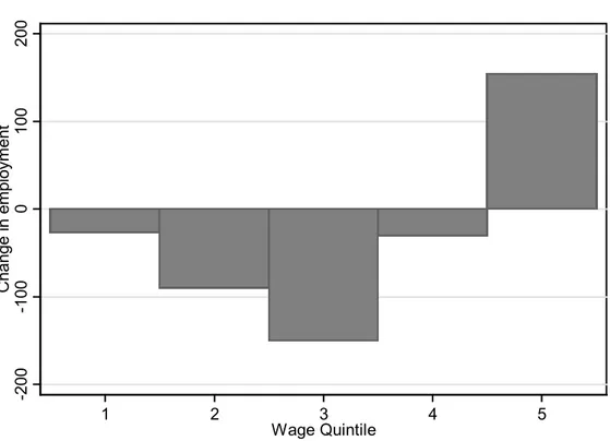
Figure 1 shows net job creation in the five wage quintiles. There is a clear pattern of polarization with most of the employment growth occurring in the highest and lowest paid jobs. Figures 2 and 3 further divide the changes into before and after 1990—the midyear in our sample. Both periods display polarization in the sense that employment in the middle quintile declines relative to jobs in the highest and lowest quintiles. On the aggregate level, the displayed changes fit well with previous knowledge about employment in Sweden, with a steady growth of the employment to population ratio up until 1990, a sharp decline in connection with the severe economic crisis of the early 1990s followed by a rebound in the late 1990s but without reaching the pre-crisis level (e.g. Holmlund, 2006).
8
Figure 1: Change in employment by wage quintiles, 1975–2005.
-100 0 100 200 300 Change in em ploy m ent 1 2 3 4 5 Wage Quintile
9
Figure 2: Change in employment by wage quintiles, 1975–1990.
0 100 200 Change in em ploy m ent 1 2 3 4 5 Wage Quintile
Changes in employment are measured in thousands of full-time equivalents
Figure 3: Change in employment by wage quintiles, 1990–2005.
-200 -100 0 100 200 Change in em ploy m ent 1 2 3 4 5 Wage Quintile
Changes in employment are measured in thousands offull-time equivalents
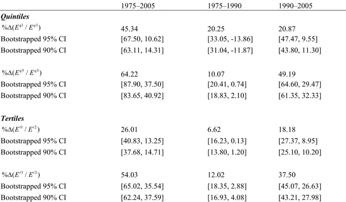
To clarify the extent of job polarization implied by Figures 1–3, the upper part of Table 1 displays the percentage changes in the ratio of employment in the first job quintile relative to the third quintile, and in the fifth quintile relative to the third quintile. That is, percentage
10
changes in (Eq1/Eq3) and (Eq5 /E , where q3) E denotes employment in the first quintile, q1 and so forth. As can be seen, between 1975 and 2005, jobs in the lowest quintile expanded by 45 percent relative to jobs in the middle quintile, with roughly equal contributions before and after 1990. The highest quintile expanded by 64 percent relative to the middle quintile over the same period, with most of the increase occurring after 1990.
Table 1: Economical and statistical significance of job polarization
1975–2005 1975–1990 1990–2005 Quintiles 1 3 % (∆ Eq /Eq) 45.34 20.25 20.87 Bootstrapped 95% CI [67.50, 10.62] [33.05, -13.86] [47.47, 9.55] Bootstrapped 90% CI [63.11, 14.31] [31.04, -11.87] [43.80, 11.30] 5 3 % (∆ Eq /Eq ) 64.22 10.07 49.19 Bootstrapped 95% CI [87.90, 37.50] [20.41, 0.74] [64.60, 29.47] Bootstrapped 90% CI [83.65, 40.92] [18.83, 2.10] [61.35, 32.33] Tertiles 1 2 % (∆ E Et / t ) 26.01 6.62 18.18 Bootstrapped 95% CI [40.83, 13.25] [16.23, 0.13] [27.37, 8.95] Bootstrapped 90% CI [37.68, 14.71] [13.80, 1.20] [25.10, 10.20] 3 2 % (∆ Et /Et ) 54.03 12.02 37.50 Bootstrapped 95% CI [65.02, 35.54] [18.35, 2.88] [45.07, 26.63] Bootstrapped 90% CI [62.24, 37.59] [16.93, 4.08] [43.21, 27.98] Note: E denotes employment in the first job quintile andq1 E denotes employment in the first job tertile; see the t1
text for details.
Previous studies in the literature on job polarization have relied on graphical analyses along the lines of Figures 1-3 without recognizing the statistical uncertainty associated with the estimated job pattern. In this study, we measure this uncertainty by applying a bootstrap procedure to the estimates in Table 1 (see e.g. Efron and Tibshirani, 1993). In the bootstrap, for each of the 1975, 1990, and 2005 samples we randomly draw n individuals with t
replacement, where n is equal to the sample size in each year t. For the 1975 bootstrap t
sample, we calculate median wages in each job and divide jobs into quintiles based on these median wages combined with the number of full time equivalent workers in each job. Changes in the number of full time jobs in each quintile is then calculated based on the bootstrap samples for each year and are used to obtain the implied percentage change in
11
1 3
(Eq /Eq ) and in (Eq5/E .q3) 5 This procedure is repeated 10,000 times and we accordingly
get 10,000 estimates of percentage changes. The bootstrap hence takes account of the uncertainty associated with estimated median wages and the number of full time workers in each job in 1975, and thereby the thresholds used to divide jobs into quintiles, as well as the uncertainty associated with the employment changes in each quintile over time.
The values corresponding to the 2.5th and 97.5th percentiles as well as the 5th and 95th percentiles in our distributions of bootstrap estimates are shown in Table 1, thus giving 95 percent and 90 percent confidence intervals. While all estimates for the periods 1975-2005 and 1990-2005 are statistically significantly different from zero, the null of a zero percentage change in (Eq1/Eq3)between 1975 and 1990 cannot be rejected. The main explanation for this is the concentration of growing jobs located just below the estimated threshold for the first quintile. When we recognize the statistical uncertainty associated with this threshold by allowing its estimate to vary over bootstrap replications, these jobs are often categorized into the second quintile, leading to lower or even negative net growth in the first quintile. Thus, the statement above of an expansion of jobs in the lowest quintile relative to the middle quintile between 1975 and 1990 is associated with a great deal of statistical uncertainty.
The statistically insignificant change in (Eq1/Eq3)prior to 1990 does not mean that there is a complete lack of statistical evidence for polarization during this period. Dividing the job ranking into tertiles (thirds) instead and using percentage changes in the first tertile (t1) relative to the second tertile, and in the third relative to the second tertile gives statistically significant estimates across the board; see the lower half of Table 1. Based on tertiles, the calculated changes still show an economically significant pattern of job polarization over the full period 1975–2005 and in the sub-period 1990–2005. However, although statistically significant, the expansion of the lowest-paying jobs (first tertile) relative to middle-paying jobs between 1975 and 1990 is now lower than seven percent.
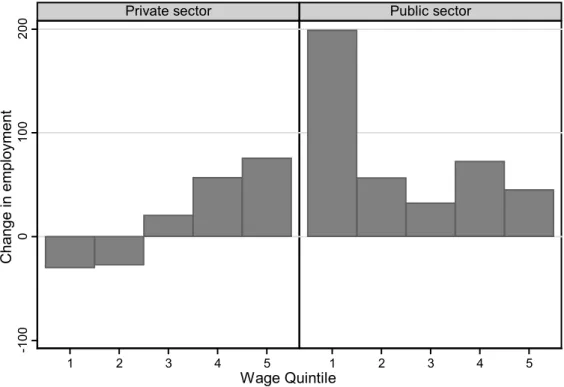
A salient feature of the Swedish labor market is the high share and marked changes of public sector employment over time; there was a marked increase from 30 percent to over 40 percent of total employment during the 1970s followed by a decline to 35 percent during the 1990s. To investigate how this fits into the overall changes in the structure of employment, Figures 4 and 5 depict the patterns in the public and private sectors separately for the periods 1975-1990 and 1990-2005, respectively. For the 1990s and 2000s, both sectors display a
5 To be consistent with the construction of our original working sample, in each bootstrap and for all years we
12
pattern that resembles the overall pattern during this period. Bootstrapped confidence intervals along the lines of those in Table 1 further confirm a statistically significant pattern of job polarization in both the public and private sectors (results are not shown but are available on request). For the earlier period, 1975–1990, the patterns are markedly different across the two sectors though. The private sector displays much smaller changes and a pattern of skill upgrading with increases in higher paying jobs at the expense of lower paying jobs, and this skill upgrading is also statistically significant. The expansion of employment in the public sector does on the other hand appear to be largely driven by low-paying jobs. A caveat with Figure 4 and the public sector, however, is the lack of any, based on bootstrapped confidence intervals, statistically significant changes (the expansion of low-paying jobs relative to middle-paying jobs borderlines significance at the 0.10-level).
Figure 4: Change in employment by sector, 1975–1990
-100
0
100
200
1 2 3 4 5 1 2 3 4 5
Private sector Public sector
Change in em
ploy
m
ent
Wage Quintile
13 Figure 5: Change in employment by sector, 1990–2005
-100
0
100
1 2 3 4 5 1 2 3 4 5
Private sector Public sector
Change in em
ploy
m
ent
Wage Quintile
Changes in employment are measured in thousands of full-time equivalents
Before we proceed to investigate the connection between changes in employment and the task contents of jobs, it is informative to see if the overall patterns of net job creation in Sweden are broadly consistent with an explanation that stresses changes in relative labor demand, as in the TBTC hypothesis, or if they are more in accord with stories that stress (exogenous) changes in labor supply. We follow Autor, Katz and Kearney (2008) and recognize that wages and employment across the job ranking are expected to covary positively (prices and quantities should change in the same direction) if changes in employment are indeed primarily driven by labor demand shifts, ceteris paribus. Like these authors, we estimate OLS regressions of the form
(1) ln p ln p p t t t t t E α β W ε ∆ = + ∆ + , where ln p t W
∆ denotes the change in the average job-specific log median wage within percentile p during period t (1975–1990 and 1990–2005). Probably because of the statistical reclassification of some jobs over time (as was discussed in Section 2), the distributions of
ln p t W ∆ and ln p t E
∆ contain some extreme values at their tails. Following the strategy employed by Autor, Katz and Kearney (2008)—who report similar problems with outliers— we base our estimations on data for the 4th through 97th percentiles of the ln p
t
W
14 ln p
t
E
∆ distributions (thus trimming outliers at the tails). We estimate β75-90 =0.53 (t-value: 0.97) for the period 1975–1990, and β90-05 =1.76 (t-value: 2.17) for the period 1990–2005. Positive changes in employment after 1990 are thus mirrored by positive changes in wages, whereas we are unable to reject a zero correlation for the earlier years. Our estimate of β75-90 is one sixth of the (positive) value obtained by Autor, Katz, and Kearney (2008) for the U.S. in the 1980s, and our estimate of β90-05 is half of their U.S. estimate for the 1990s. Our point estimate for 1990–2005 is, however, larger than the corresponding estimate for the former West Germany in Dustmann, Ludsteck and Schönberg (2009), whereas the point estimate for the earlier period is of similar magnitude. As a sensitivity analysis, we have also used data for the 10th through 91st percentiles in the employment and wage distributions. We then estimate
75-90 1.59
β = − (t-value: 1.94) and β90-05 =2.18(t-value: 2.86); hence, trimming the tails further yields different result for the period 1975–90 but strengthens those for the period 1990–2005. Given the strong evidence for job polarization between 1990 and 2005, these estimates are consistent with a story that stresses relative demand shifts in favor of low-wage and high-wage workers relative to middle-high-wage workers during this period.6 This is however not the
case for the earlier period.
3.2 The importance of routine versus nonroutine tasks
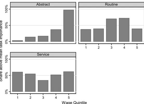
Is there any connection between the patterns of net job creation and the extent of routine and nonroutine tasks across the job distribution, and does it fit the predictions of TBTC? As a first overview, Figure 6 displays the share of workers in each wage quintile in 1975 that are in an occupation with a task score on abstract, routine and service above the overall mean. As can be seen, abstract tasks are more important in the highest paid jobs and service tasks are most important at the very highest and lowest paid jobs, whereas routine tasks are least important in the tails of the distribution. This mirrors previous documentations for the U.S. and U.K.
6 Note, however, that the estimates do not automatically translate into decreased wage differentials in the lower
half of the wage distributions or increased differentials in the upper half since one also needs to take into account the changing composition of jobs as well as changes in wage dispersion within jobs (see Goos and Manning, 2007). In fact, although the Swedish 90/50-quotient did indeed increase during the 1990s, the 50/10-quotinent also increased during the same period, albeit less so (Gustavsson, 2006; Domeij, 2008). According to the results in Nordstrom-Skans, Edin and Holmlund (2009), the rise in the Swedish 50/10-quotinent is consistent with increased wage dispersion within jobs.
15
Figure 6: Incidence of abstract, routine, and service tasks across wage quintiles
0% 50% 100% 0% 50% 100% 1 2 3 4 5 1 2 3 4 5 Abstract Routine Service S har e abov e m ean t as k im por tan ce Wage Quintile
Note: The figures display the share of workers in each job/wage quintile that are in an occupation with a task score above the overall mean. The underlying task scores are from Goos, Manning, and Salomons (2009)
Based on simple “eye-ball econometrics”, the distributions of job tasks in Figure 6 combined with our documentation of job patterns in the previous sub-section speaks against TBTC along the line of ALM as an important factor between 1975 and 1990. During this period, the private sector displays a clear pattern of skill upgrading, with monotone increases in higher paying jobs at the expense of lower paying jobs; see Figure 4. Hence, combined with Figure 6, this indicates that low-paid service jobs, rather than middle-paid routine job as predicted by ALM, experienced the weakest job growth in the private sector prior to 1990.
We have also redone the analysis in Figure 6 using the five related routine and nonroutine task measures developed by Autor, Levy and Murnane (2003).7 These are derived from much less information than those of Goos, Manning, and Salomons (2009) but make it possible to investigate potential changes in jobs tasks over time since there are two versions of each measure, one created from information about job tasks in 1977 and one based on information from 1991. These alternative measures do not change any conclusions related to the distribution of routine versus nonroutine tasks and they do not generally indicate marked
16
changes in the extent of routine versus nonroutine content of jobs over time (results are available on request).
As a more stringent analysis of the connection between changes in employment and job tasks, we next regress changes in job-specific employment on the three task measures. Since we have a lot of small jobs where measurement errors are expected to be large, we only include jobs with at least ten employees in all three years 1975, 1990 and 2005; including all jobs in the regression analysis gives similar point estimates but substantially larger standard errors. Though we lose a lot of jobs by this restriction, we still retain 95 percent of all individuals in 1975 (93 percent in 1990, and 92 percent in 2005).
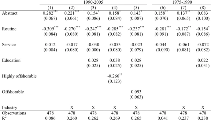
The first five columns of Table 2 contain results for the period 1990-2005. The explanatory variables in the first column are the three task-measures in the form of dummy variables that equal unity for occupations with scores above the overall mean. The estimates corroborate the impression from Figures 3 and 6 and are broadly consistent with the routinization hypothesis; there is a statistically significant expansion of jobs intense in
abstract tasks, a statistically significant decline in jobs intense in routine tasks, and no
statistically significant change for jobs intense in service tasks.
However, a serious investigation of how job tasks covary with changes in employment—related to the TBTC hypothesis—should try to control for changes in employment that stem from changes in product demand. That is, jobs that are intense in routine tasks may have declined in employment simply because these jobs are concentrated in industries with falling product demand and not necessarily because of organizational changes. To try to control for this, in the second column we add dummy variables for the 31 industries used to define a job (two letter level SNI). The results show a statistically significant positive effect of abstract and a statistically significant negative effect of routine also within industries. Hence, industry-specific changes in employment are not behind the decline of routine jobs in Sweden after 1990.
The third column of Table 3 further adds the mean number of years of schooling (education) in each job in 1975 as a regressor. As argued by Goos, Manning and Salomons (2009, 2010), this variable allows for the predictions from the traditional SBTC hypothesis where employment should simply increase for jobs that require more education (more skills) relative to jobs that demand less education (less skills). As can be seen, education is not statistically significant and does not change any conclusions whereas abstract is still significantly positive (at the 0.10 level) and routine is still significantly negative.
17
In the U.S., it has been argued that the decline of routine jobs in the middle of the wage distribution could be due to increased offshoring of jobs, that is, the migration of employment from the home country to other (mostly poorer) countries, rather than due to substitution between labor and computers along the lines of ALM (see e.g. the discussion in Acemoglu and Autor, 2011). There is a lack of data on the number of jobs actually offshored for most countries, but recent attempts to classify the offshorability of jobs— the ability to perform the work duties from abroad—by Blinder (2009) and Blinder and Krueger (2010) actually suggest that there is no correlation between the extent of routine tasks in a job and its offshorability. For instance, Blinder and Krueger (2010, p.38) conclude that “routine work is no more likely to be offshorable than other work”.
To see if the offshorability of jobs could still potentially change any of our conclusions for the period 1990–2005, we use Blinder’s (2009) classification of a job’s offshorability, which in turn is based on information in the U.S. O*NET database. Blinder (2009) categorizes jobs into one of four levels of offshorability: 1) Highly offshorable (a person in this job does not have to be physically close to a work unit, e.g. computer programmers and telemarketers); 2) Offshorable (the whole work unit could be moved abroad, e.g. most factory workers); 3)
Non-offshorable (whole work unit must be in home-country, e.g. sales managers), 4) Highly non-offshorable (e.g. child-care workers and farmers). The reader is referred to Blinder’s
study for more information on the criteria underlying this classification.
In the fourth column of Table 3 we include, for the period 1990–2005, a dummy variable for jobs that are judged to be highly offshorable. This variable is negative and statistically significant, but its inclusion does not change the results for the other variables. A dummy for all jobs that are offshorable (which includes highly offshorable jobs) is insignificant, and other estimates are unchanged. Based on this, combined with previous studies in the literature, we find it unlikely that offshoring can explain the polarization of the Swedish labor market between 1990 and 2005. Overall, our set of regressions for the period 1990–2005 are broadly in line with the results for Western Europe in Goos, Manning, and Salomons (2009, 2010).
We next present regression results for the period 1975–1990. The last three columns of Table 3 present specifications with, first, the three task measures as the only regressors, then with industry dummies added, and finally also with the inclusion of average educational attainment in 1975. As expected, the evidence for routinization is weaker compared to the period 1990–2005, although not absent. The estimates for abstract and routine are statistically significant and with the correct sign in the first two regressions, whereas only routine is
18
statistically significant (at the 0.10 level) once education is controlled for. The share of the total variation explained by the three task measures is lower for this period; the R2 with only the three task dummies is less than half of that for 1990–2005 and the partial R2 for these three task measures when industry dummies are included is also three times smaller for the period 1975–1990, with a value of 0.06 for 1990–2005 versus 0.02 for 1975–1990.8
We have also included the variables offshorable and highly offshorable for the period 1975-1990 (not shown). Their estimates are positive and statistically significant, without affecting the estimates for the other variables. A possible explanation for the positive estimates is the fact that Blinder’s (2009) measures are created with modern information technology in mind, and thus may be a bad proxy for the offshorability of jobs prior to the 1990s.
Table 2: OLS regressions; log change in job-specific employment
1990-2005 1975-1990 (1) (2) (3) (4) (5) (6) (7) (8) Abstract 0.282*** 0.221*** 0.154* 0.158* 0.143* 0.158** 0.137** 0.083 (0.067) (0.061) (0.086) (0.084) (0.087) (0.070) (0.065) (0.100) Routine -0.309*** -0.270*** -0.247*** -0.285*** -0.237*** -0.281*** -0.172** -0.154* (0.084) (0.080) (0.081) (0.082) (0.081) (0.091) (0.087) (0.086) Service 0.012 -0.017 -0.030 -0.053 -0.023 -0.044 -0.061 -0.072 (0.084) (0.080) (0.080) (0.080) (0.079) (0.090) (0.081) (0.082) Education 0.028 0.038 0.028 0.022 (0.025) (0.025) (0.025) (0.031) Highly offshorable -0.266** (0.123) Offshorable 0.093 (0.063) Industry X X X X X X Observations 478 478 478 478 478 478 478 478 R2 0.086 0.260 0.262 0.269 0.265 0.041 0.237 0.238
Note: Dependent variable is log change in job-specific employment. Robust standard errors are in parentheses. Regressors are dummy variables equal to one if the skill measure for a job is above the mean. Education is mean education in a job in 1975.
* p < 0.10, ** p < 0.05, *** p < 0.01
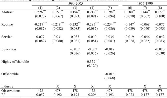
The longitudinal dimension of our data also allows us to investigate if individual job mobility is in the direction away from routine jobs. To do this, we re-estimate the regression in Table 3 but only base the calculation of the dependent variable on those individuals that held a job in both the start and end of the investigated periods. Changes in job-specific
8 This is the same kind of partial R2 used in Acemoglu and Autor (2010). A formula and explanation can be
19
employment—the dependent variable—can hence only be driven by differences in the extent of job mobility to and from different kinds of jobs, and not by entries and exits from the labor market/employment. That is, changes in the composition of the labor force will not affect the estimates, like for instance the large inflow of immigrants into Sweden during the studied period and the large expansion of female labor force participation during the 1970s and 1980s.
As can be seen, the longitudinal estimates for the period 1990–2005 are similar to those for the cross-sectional estimates in Table 2 and imply statistically significant individual job mobility away from jobs with routine tasks toward jobs with abstract tasks, even when mobility between industries are accounted for. This constitutes additional evidence in favor of TBTC along the lines of ALM as an important explanation for the 1990s and 2000s. This conclusion, however, does not carry over to the estimates for 1975–1990. In particular, the estimate for routine is not statistically significant when we control for industry-specific effects. We are hence not able to reject the hypothesis that the expansion of certain industries, rather than organizational changes within industries, can account for mobility away from routine jobs during this period.
Table 3: OLS regressions; longitudinal changes in job-specific employment
1990-2005 1975-1990 (1) (2) (3) (4) (5) (6) (7) (8) Abstract 0.226*** 0.157** 0.196** 0.212** 0.198** 0.180** 0.144** 0.168* (0.070) (0.067) (0.093) (0.091) (0.094) (0.070) (0.067) (0.100) Routine -0.217*** -0.218*** -0.232*** -0.285*** -0.234*** -0.147* -0.068 -0.077 (0.082) (0.082) (0.085) (0.087) (0.086) (0.089) (0.090) (0.093) Service 0.077 0.031 0.037 0.010 0.035 -0.019 -0.046 -0.042 (0.082) (0.080) (0.081) (0.081) (0.081) (0.088) (0.082) (0.083) Education -0.017 -0.007 -0.017 -0.010 (0.026) (0.026) (0.026) (0.030) Highly offshorable -0.359*** (0.120) Offshorable -0.016 (0.068) Industry X X X X X X Observations 478 478 478 478 478 478 478 478 R2 0.057 0.192 0.193 0.206 0.193 0.023 0.177 0.177
Note: Dependent variable is log change in job-specific employment for individuals with employment in both 1975 and 1990, and in both 1990 and 2005. Robust standard errors are in parentheses. Regressors are dummy variables equal to one if the skill measure for a job is above the mean. Education is mean education in a job in 1975.
20
Given the results in Tables 2 and 3, a relevant question is how much of the observed job polarization between 1990 and 2005 that can potentially be explained by TBTC along the lines of ALM. To investigate this, we use the estimates in Table 2 to calculate the degree of polarization that would remain if all jobs had the same extent of routine and non-routine tasks. That is, how much of the polarization will remain if we assume that all jobs have zeros on the dummy variables abstract, routine, and service? These are obviously back-of-the-envelope calculations since they discard any kind of general equilibrium effects and are based on rather explorative estimates. But we still believe that they, at the very least, should be able to give an idea of the importance of routinization.
As our measures of polarization, we use the percentage change in the ratio of employment in the first quintile relative to the third quintile, (Eq1/Eq3), and in the fifth quintile relative to the third quintile—the same measures that were discussed in connection with Table 1. To calculate the counterfactual extent of polarization that would remain if all jobs had the same extent of routine and non-routine tasks, we first convert the estimates in Table 2 for abstract and routine into the implied percentage effects (the anti-log of the estimate minus unity); we do not use the estimate for service since it is statistically insignificant. Denote these percentage effects for abstract and routine by γa and γ , r
respectively. To obtain a counterfactual value for employment in the first quintile in 2005, denoted 1
05q
E , we subtract the change in employment since 1990 associated with the extent of
routine and abstract tasks in the first quintile from the actual value of 1
05q
E , using the formula
(2) 1 1 1 1 1
05q 05q 90q ( r q a q )
E =E −E γ ⋅routine + ⋅γ abstract ,
where routine is the mean value of routine in the first quintile, i.e. the share of employment q1 in the first quintile with the dummy variable routine equal to unity. That is, in equation (2), the positive change in employment between 1990 and 2005 associated with abstract tasks in the first quintile is removed, as is the negative effect associated with routine tasks. What is left is the level of employment in the first quintile in 2005 that would exist if all jobs had the same task content (as measured by the dummy variables abstract and service). The corresponding calculation is done for the other quintiles. To obtain a counterfactual value of polarization between 1990 and 2005, we then use the resulting values of 1
05q
E and 3
05q
E in the calculation of percentage changes in the ratio of employment in the first job quintile relative
21
to the third quintile, calculated as 1 3 1 3 1 3
05 05 90 90 90 90
[(Eq /Eq ) (− Eq /Eq )] / (Eq /Eq ), and so forth for the earlier period and for changes in employment in the fifth relative to the third quintile.
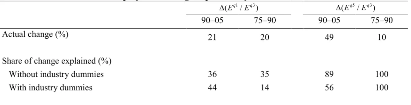
Between 1990 and 2005, the actual increase of employment in the fifth relative to the third quintile was 49 percent, i.e. (Eq5/E increased by 49 percent. Based on the estimates q3) for abstract and routine in the specification with only the three task dummies in the first column of Table 2 and the formula in equation (2), the counterfactual increase in (Eq5 /E q3) is 5.3 percent. That is, when we replace the actual values of 3
05q E and 5 05q E by their counterfactual values 3 05q E and 5 05q
E that are cleansed of the impact of job tasks, we observe a much smaller growth of the fifth relative to the third quintile. In fact, the obtained number implies that the distribution of tasks can potentially account for 89 percent (1-5.3/49) of the actual percentage increase in (Eq5/E ; see Table 4. When we instead use the estimates for q3) abstract and routine from the specification with industry-specific effects in the second
column of Table 2, we get a counterfactual increase in (Eq5/E of 21.5 percent. This q3) means that the share of the actual increase explained by job tasks decreases to 56 percent (1-21.5/49) once we take industry effects into account. For the period 1975–1990, we obtain negative counterfactual percentage changes in (Eq5/E , so tasks can potentially account q3) for all of the—moderate—actual increase in (Eq5/E between 1975 and 1990. q3)
We next turn to the explanatory power of tasks for changes in (Eq1/Eq3), which we view as the most interesting exercise since the stand-out prediction of the TBTC hypothesis— compared to that of traditional SBTC—is the expansion of the lowest-paid jobs relative to middle-paid jobs. Based on the specification with only the three task dummies in the first column of Table 3, for the period 1990–2005 we find, using the same methodology as above, that the distribution of tasks can account for 36 percent of the actual increase in (Eq1/Eq3). Using estimates from the specification with industry-specific effects in the second column raises the share explained further, to 44 percent. For the period 1975–1990, the specification with only the three tasks measures can potentially account for 35 percent of the (statistically insignificant) actual increase in (Eq1/Eq3). Taking industry effects into account does however markedly lower the explanatory power to 14 percent for the period 1975–1990.
22
Table 4: Share of relative employment change explained by task content 1 3
(Eq /Eq )
∆ ∆(Eq5/Eq3) 90–05 75–90 90–05 75–90
Actual change (%) 21 20 49 10
Share of change explained (%)
Without industry dummies 36 35 89 100
With industry dummies 44 14 56 100
Note: The share of change explained is calculated based on regression estimates in Table 2; see the text for details.
4. Concluding remarks
This paper documents a pattern of job polarization in Sweden between 1975 and 2005 with increased employment shares of the highest and lowest paid jobs. Unlike the polarization after 1990, the pattern of net job creation between 1975 and 1990 is however associated with a great deal of statistical uncertainty. We are also unable to find consistent evidence in favor of TBTC as a major explanation for the pattern of net-job creation prior to 1990. Investigations of changes after 1990 are on the other hand fully consistent with the TBTC hypothesis. In line with a demand-side explanation, there is a statistically significant positive correlation between changes in employment and wages across the job distribution after 1990. Regression estimates for the same period indicate increased employment in jobs that require cognitive nonroutine skills and decreased employment in jobs that primarily require routine skills, and an analysis based on longitudinal data displays the same pattern for individual job mobility. In total, our analysis combined with back-of-the-envelope calculations suggests that the distribution of routine and nonroutine tasks across the job distribution can account for 44 percent of the observed rise in low-wage relative to middle-wage employment after 1990 but largely lacks explanatory power in earlier years.
Our findings for Sweden add to the notion of TBTC along the lines of ALM as a real phenomenon across a wide range of countries during the 1990s and 2000s. In particular, while most of the previous evidence for job polarization applies to the U.S. and U.K., our evidence, combined with the overview of job patterns across Europe in Goos, Manning and Salomons (2009), suggest that the TBTC hypothesis is consistent with the pattern of net job creation across countries with markedly different institutional settings.
Our lack of consistent support for the TBTC hypothesis during the period 1975–1990 fits well with Autor, Katz and Kearney’s (2009) result for the U.S., where a pattern of job
23
polarization is found for the 1990s but not for the 1980s. These common results point toward the 1990s as the decade when computerization of the workplace may have started to have a significant bearing on employment in routine jobs. Not much is however known about such organizational changes or their exact timing, so this is clearly an area that warrants more research.
24 References
Acemoglu, D. (2001), “God Jobs versus Bad Jobs”, Journal of Labor Economics 19, 1–21. Acemoglu, D. (2003), “Cross-Country Inequality Trends”, Economic Journal 113, 121–149. Acemoglu, D. and D. Autor (2011), “Skills, Tasks and Technologies: Implications for
Employment and Earnings”, in O. Ashenfelter and D. Card (eds.), Handbook of Labor
Economics Volume 4, Elsevier Science B.V., Amsterdam.
Atkinson, A. (2008), The Changing Distribution of Earnings in OECD Countries, Oxford University Press, Oxford.
Autor, D. and D. Dorn (2010), “The Growth of Low-Skill Service Jobs and the Polarization of the U.S. Labor Market”, MIT Working Paper.
Autor, D., L. Katz, and M. Kearney (2008), “Trends in U.S. Wage Inequality: Re-Assessing the Revisionists”, Review of Economics and Statistics 90, 300–323.
Autor, D., F. Levy and R. Murnane (2003), “The Skill Content of Recent Technological Change: An Empirical Exploration”, Quarterly Journal of Economics 118, 1279–1333.
Björklund, A. and R. Freeman (2010), “Searching for Optimal Inequality/Incentives”, in R. Fremman, B. Swedenborg and R. Topel (eds.), Reforming the Welfare State: Recovery
and Beyond in Sweden, The University of Chicago Press, Chicago.
Blinder, A. (2009), “How Many U.S. Jobs Might be Offshorable?”, World Economics 10, 41–78
Blinder, A. and A. Krueger (2010), “Alternative Measures of Offshorability: A Survey Approach”, forthcoming in Journal of Labor Economics.
Cahuc, P. and Zylberberg, A. (2004), Labor Economics, MIT Press, Cambridge.
Domeij, D. (2008), “Rising Earnings Inequality in Sweden: The Role of Composition and Prices“, Scandinavian Journal of Economics, 110, 609–634.
Dustman, C., J. Ludsteck and U. Schönberg (2009), “Revisiting the German Wage Structure”,
Quarterly Journal of Economics 124, 843–881.
Edin, P.-A. and P. Fredriksson (2000), “LINDA – Longitudinal Individual Data for Sweden”, Working Paper 2000:19, Department of Economics, Uppsala University.
Efron, B. and R. Tibshirani (1993), An Introduction to the Bootstrap, Chapman and Hall, New York..
25
Fernández-Macías, E. and J. Hurley (2008), “More and Better Jobs: Patterns of Employment Expansion in Europe”, The European Foundation for the Improvement of Living and Working Conditions, ERM Report 2008.
Goos, M. and A. Manning (2007), “Lousy and Lovely Jobs: The Rising Polarization of Work in Britain”, Review of Economics and Statistics 89, 119–133.
Goos, M., A. Manning and A. Salomons (2009), “Job Polarization in Europe”, American
Economic Review: Papers & Proceedings 9, 58–63.
Goos, M., A. Manning and A. Salomons (2010), “Recent Changes in the European Employment Structure: The Roles of Technology and Globalization”, mimeo, University of Leuven.
Gustavsson, M. (2006), "The Evolution of the Swedish Wage Structure: New Evidence for 1992-2001", Applied Economics Letters 13, 279-286.
Holmlund, B (2006), “The Rise and Fall of Swedish Unemployment”, in M. Werding (ed.),
Structural Unemployment in Western Europe: Reasons and Remedies, MIT Press,
Cambridge.
Katz, L. and D. Autor (1999), “Changes in the Wage Structure and Earnings Inequality” in O. Ashenfelter and D. Card (eds), Handbook of Labor Economics, Vol. 3A, Elsevier Science B.V., Amsterdam.
Kennedy, P. (1998), A Guide to Econometrics, Blackwell, Oxford.
Nordstrom-Skans, O., P.-A. Edin and B. Holmlund (2009), "Wage dispersion between and within plants:Sweden 1985-2000" in Lazear E & K Shaw (eds) The Structure of
Wages: An InternationalComparison, University of Chicago Press, Chicago
Statistics Sweden (1977), Swedish Standard Industrial Classification of all Economic
Activities. Reports on Statistical Co-ordination 1977:9, Stockholm.
Statistics Sweden, (1984), Population and Housing Census 1980. Part 9. Occupation, Stockholm.
Statistics Sweden (1989), Occupations in the Population and Housing Census 1985 (FoB 85)
according to Nordic standard occupational classification (NYK) and Swedish socio-economic classification (SEI). Reports on Statistical Co-ordination 1989:5,
Stockholm.
Statistics Sweden, (1992) Swedish Standard Industrial Classification 1992. Reports on
Statistical Co-ordination 1992:6, Stockholm.
Statistics Sweden (1998), Standard Classification of Occupations 1996. Reports on Statistical
Co-ordination for the Official Statistics of Sweden 1998:3, Stockholm.
Statistics Sweden (2003), Swedish Standard Industrial Classification 2002. Reports on
26
Wright, E. O. and R. Dwyer (2003), “The Patterns of Job Expansion in the USA: A Comparison of the 1960s and 1990s”, Socio-Economic Review 1, 289–325.
Åberg, R. (2004), “Vilka jobb har skapats på den svenska arbetsmarknaden de senaste decennierna?”, Ekonomisk debatt 32(7), 37–46.
27 Appendix
Data sources and sample
We use three years of LINDA data: 1975, 1990 and 2005. For the 1975 and 1990 samples, information on occupation, industry and sector as well as hours worked comes from the Population and Housing Censuses (FoB). For the 2005 samples, we use information from the LINDA Wage Survey. The classification schemes for occupation and industry have changed several times in Sweden, so in order to study changes in jobs we need to translate the older schemes into those used in our 2005 data. The detailed procedures for this are described below.
We keep all persons of ages 18-64 and drop those with missing values on occupation, industry, sector or work hours. The sample sizes are shown in Table A1.
Table A1: Sample sizes
1975 1990 2005
Initial sample 220,795 240,689 132,806
Ages 18-64 165,279 174,493 132,720
Non-missing occupation, industry, sector and work hours, ages 18-64 123,080 124,120 117,535
We define a job as a unique combination of an occupation and an industry. We use three-digit SSYK coding for occupation (described in detail below), resulting in 113 categories, and for industry we use two-letter SNI 2002 (described in detail below), resulting in 31 categories. Interacting these creates 3,503 possible jobs. Not all occupations, industries or jobs are represented in our data. In the 1975 sample we observe 94 occupations, 31 industries and 1 377 jobs, in the 1990 sample we observe 112 occupations, 31 industries, and 1,958 jobs, and in the 2005 sample we observe 113 occupations, 29 industries and 1,669 jobs. New jobs (jobs that were empty in the 1975 sample) are dropped; see the main text for a discussion of this. There are 744 new jobs in the 1990 sample and 161 new jobs in the 2005 sample.
To perform our analysis, we need to construct full-time equivalent “individuals” from our actual individuals, many of whom work part-time. The 1975 and 1990 samples only include categorical information on hours worked, while the 2005 sample contains information on actual hours. For comparability, we collapse work hour information to four categories in all samples. For each category we then calculate mean hours worked from the 1974 edition of the Swedish Level of Living Survey (LNU)9, as this data set includes data on hours worked.
28
We then assign these means (10 hours for the 1-15 hours category, 17 hours for the 16-19 hours category, 24 hours for the 20-34 hours category and 40 hours for the 35-40 hours category) to the individuals in each category in our three samples.
Occupational coding
Official Swedish occupational statistics use the Swedish Standard Classification of Occupations 1996 (SSYK), which is a four-level hierarchical scheme with 10 major groups (listed in Table A2), 27 sub-major groups, 113 minor groups and 355 unit groups. SSYK is based on the International Standard Classification of Occupations 1988 (ISCO-88) published by the International Labour Organization and on the European Union version ISCO-88(COM), with some adjustments for the Swedish labor market. SSYK replaced the earlier Nordic Standard Occupational Classification 1983 (NYK83) scheme, which was based on ISCO-58 (Statistics Sweden 1998).
Table A2: Swedish Standard Classification of Occupations (SSYK) Code Major groups
1 Legislators, senior officials and managers 2 Professionals
3 Technicians and associate professionals 4 Clerks
5 Service workers and shop sales workers 6 Skilled agricultural and fishery workers 7 Craft and related trades workers
8 Plant and machine operators and assemblers 9 Elementary occupations
In the Population and Housing Censuses (FoB), however, other classification schemes were used. FoB 75 and FoB 80 used identical schemes, YK80, based on NYK78 (Statistics Sweden 1984). FoB 85 and FoB 90 used a version of NYK83, YK85, documented in Statistics Sweden (1989). FoB 85 also provides a YK80 code for each individual, so that occupation is registered using both the older and newer schemes. Statistics Sweden have constructed a detailed translation key for going from three-digit YK80 and three- or five-digit YK85 to one-, three- or four-digit SSYK. The key is one-to-one for going from YK85 to SSYK, but for some YK80 codes there are several possible SSYK codes. The key, however, also contains head counts from 1985 and 1990 censuses. For each ambiguous YK80 code, we pick the SSYK code that is most frequent in the 1985 census.
We use this key to recode the 1975 occupation variable from digit YK80 to digit SSYK, and for recoding the 1990 occupation variable from five-digit YK85 to three-digit SSYK. Some occupations, however, are not translated by the key. In the 1975 data, 25
29
occupations are not translated. We drop those occupations with less than 20 observations, leaving us with one occupation. We then exploit the panel structure in LINDA and the double coding in FoB 85 by tabulating the YK85 occupation codes from the 1985 cross section for the untranslated occupation in 1975. We then assign the most frequent YK85 code to this YK80 code. The YK85 code is then translated to SSYK using the more detailed YK85 to SSYK key. In this case 41 percent of observations are found in the most frequent YK85 code, while only 6 percent are in the second most frequent YK85 code. We drop 89 observations in 23 occupations having less than 20 observations, and we drop 197 observations having the code for indefinable occupations in YK80.
For the 1990 occupation variable, we use the Statistics Sweden key to go from five-digit YK85 to three-digit SSYK. We drop 4 646 observations, of which 1 119 have the code for unidentifiable occupations in YK85, and 3 526 are marked as untranslatable in the Statistics Sweden key.
Industry coding
Official Swedish industry statistics uses the Swedish Standard Industrial Classification (SNI), the latest version being SNI 2007. We use the earlier SNI 2002 scheme, however, since the 2005 sample uses this scheme. SNI 2002 is a hierarchical six level scheme, with 17 one-letter sections (listed in Table A3), 31 two-letter sub-sections, 60 two-digit main groups, 222 three-digit groups, 513 four-three-digit sub-groups, and 776 five-three-digit detailed groups. SNI 2002 is identical to the Statistical Classification of Economic Activities in the European Communities (NACE) Rev 1.1 published by the European Union at the four-digit level, while the five-digit level does not exist in NACE. SNI 2002 replaced the similar SNI 92, which was based on NACE Rev 1 (Statistics Sweden 1992; 2003). NACE Rev 1 was in turn based on the International Standard Industrial Classification of All Economic Activities (ISIC) Rev 3, published by the United Nations.
Table A3: Swedish Standard Industrial Classification (SNI 2002) Code Sections
A Agriculture, hunting and forestry B Fishing
C Mining and quarrying D Manufacturing
E Electricity, gas and water supply F Construction
G Wholesale and retail trade; repair of motor vehicles, motorcycles and personal and household goods H Hotels and restaurants
I Transport, storage and communication J Financial intermediation