Alterations in the Liquidity Premium as an Effect of Exchange Traded Funds : A Study Performed on Nasdaq Composite between 1997 and 2016

(1)

ALTERATIONS IN THE LIQUIDITY

PREMIUM AS AN EFFECT OF EXCHANGE

TRADED FUNDS

A STUDY PERFORMED ON NASDAQ COMPOSITE

BETWEEN 1997 AND 2016

MASTER THESIS WITHIN BUSINESS ADMINISTRATION

THESIS WITHIN: Finance NUMBER OF CREDITS: 30 ECTS

PROGRAMME OF STUDY: Civilekonomprogrammet AUTHORS: Andersson, Axel & Svanberg, Emanuel TUTOR: Stephan, Andreas

(2)

Master Thesis within Business Administration

Title: Alterations in the Liquidity Premium as an Effect of Exchange Traded Funds A Study Performed on NASDAQ Composite Between 1997 and 2016 Authors: Andersson, Axel & Svanberg, Emanuel

Tutor: Stephan, Andreas Date: 2018-05-17

Key Terms: Liquidity Premium, Characteristic Liquidity, Systematic Liquidity, Indexation, Exchange Traded Funds, Fama-MacBeth Regression

Abstract

Investors have historically demanded a return premium for taking on the risk of illiquidity both in terms of characteristic and systematic liquidity risk. Recent research have presented results suggesting that the liquidity premium is diminishing. The increasing popularity of passive investments such as Exchange Traded Funds (ETFs) have been proposed as a driving force for the declining trend. Despite the popularity of ETFs, there is limited research how they impact the financial markets. The purpose of this thesis is to investigate how the liquidity premium has developed in the United States between 1997 and 2016 and to explore if developments in the liquidity premium can be linked to the capital inflow to the United States ETF market. The thesis uses measures of stocks’ spreads and order book depths as proxies for the characteristic and systematic liquidities. The proxies are used to test if liquidity has influenced stock returns over 1-year, 5-years and the entire 20-year period. The empirical results obtained through Fama-MacBeth regressions show that the liquidity premium can fluctuate by both sign and magnitude year by year. The characteristic risk premium is negative and significant for the entire 20-year period and the 1-year regressions suggests a clear negative trend. The systematic liquidity premium on the other hand is positive and significant for the entire 20-year period but the 1-year regressions do not show a clear trend. The empirical results show no statistical significance that ETFs influence the liquidity premium. However, the graphical interpretation of the 1-year regressions suggests that the characteristic liquidity premium is negatively correlated with the growth of ETFs. The negative characteristic premium implies that investors are not being adequately compensated for the risk of illiquidity and should therefore avoid a liquidity-based investing strategy which has generated excess return in the past.

(3)

Tables

TABLE 1:LIQUIDITY PROXIES USED IN DIFFERENT STUDIES ... 8

TABLE 2:DESCRIPTIVE STATISTICS STOCKS ... 23

TABLE 3:DESCRIPTIVE STATISTICS PORTFOLIOS ... 23

TABLE 4:BREUSCH-PAGAN TESTS ... 26

TABLE 5:WOOLDRIDGE TEST ... 27

TABLE 6:20-YEAR REGRESSION ... 28

TABLE 7:5-YEAR REGRESSIONS ... 28

TABLE 8:1-YEAR REGRESSIONS SPRPT ... 29

TABLE 9:1-YEAR REGRESSIONS DPTPT ... 30

TABLE 10:INPUTS USED IN THE TIME-SERIES REGRESSIONS TO ESTIMATE ETFS IMPACT ON THE LIQUIDITY PREMIUM ... 31

TABLE 11:REGRESSION OUTPUT BASED ON THE INPUT FROM TABLE 10 ... 32

TABLE 12:RAMSEY RESETTEST ... 33

Figures

FIGURE 1:CHARACTERISTIC LIQUIDITY PREMIUM TREND ... 35

FIGURE 2:SYSTEMATIC LIQUIDITY PREMIUM TREND ... 35

FIGURE 3:RELATIONSHIP ETF AND SPR ... 37

(5)

1

Introduction

This chapter introduce the reader to the subjects of the thesis: the liquidity premium and exchange traded funds as well as to the problem and purpose. In the end of the chapter, two research questions are stated which are investigated further in the thesis.

Background

The liquidity premium is a central concept in equity pricing theory. Essentially, the liquidity premium is a return premium demanded by investors for holding illiquid assets. Equities with low liquidity are characterized by higher trading costs due to their wider bid-ask spreads (Amihud & Mendelson, 1986a). As a result of the higher trading cost, investors require a higher return from these investments. Historically, equities with less market liquidity have generated a better return than equities with more liquidity over time (Amihud & Mendelson, 1986b). Because the financial market has evolved since the first discovery of the premium it is of interest to investigate how the premium has developed in recent years.

A noticeable development on the market is the surge of capital into passive investing. The financial market has experienced a shift in capital allocation, from active management to passive management (Investment Company Institute [ICI], 2017). One kind of a passive investment that have gained ground are index funds. The goal of an index fund is to mimic a specified benchmark. The assets in index funds have grown from $11 million in 1975 to $4 trillion in late 2015, representing 34% of the equity funds’ market (Bogle, 2016). The rise in popularity of passive investments may be credited to the debate whether active fund managers can generate a better return than a passive index over time, and hence justify a management fee (Frino, Gallagher & Oetomo, 2005).

There are two different types of index funds: mutual index funds and Exchange Traded Funds (ETFs). This study focus on ETFs because of their increasing popularity and because of how they are structured. However, a section with a discussion and comparison of selected features between ETFs and mutual index funds is included. ETFs have gained much attention due to their low fees and their ability to be traded intra-daily on a stock exchange. The net assets of the United States ETF market have grown from $7 billion in 1997 to more than $2,500 billion in 2016 (ICI, 2017). An important distinction between mutual index funds and ETFs is that the price of an ETF is determined by the market participants. To keep the ETF price in line with the Net Asset Value (NAV) of the underlying components, the issuer of an ETF authorizes an external partner to create and redeem ETF shares in exchange for these components. The external partners are called Authorized Participants (APs) and are typically large institutions. When the price of an ETF is above the NAV of the underlying equities the AP buys the securities and create new ETF shares pushing the price of the securities up and the price of the ETF

(6)

2

down. If an ETF is priced at a discount the AP buys the ETF and redeem it with the issuer which pushes the price up (ICI, 2017).

When large amounts of capital are being transferred between different securities it could impact their valuations. Coval and Stafford (2007) conducted a study on asset fire sales and purchases and found that underlying securities in a fund that had large out(in)flows experienced a negative (positive) price pressure. In the case of ETFs, this indicates that the valuations of the underlying securities are affected due to the massive capital inflows to these funds. A consequence of this could be that equities which are overrepresented in ETFs have their valuations positively skewed compared to equities underrepresented in ETFs.

ETF funds’ performances can be evaluated by assessing their tracking error. The tracking error is a measurement of how well a fund has been able to track its benchmark. The presence of illiquid stocks in the benchmark can make it harder to achieve a good tracking error. This is due to their wider bid-ask spread which increases the cost for the fund (Buetow & Henderson, 2012). Hence, an underrepresentation of illiquid stocks is expected in ETFs. The existence of ETF issuers’ ability to “sample” their holdings strengthens the argument. Sampling means that they have the right to choose a representative basket from an index while excluding certain components. It is common to exclude illiquid stocks that would be costly to include (Buetow & Henderson, 2012; Maurer & Williams, 2015). ETF issuers have to assess what impair the tracking error most: 1) Including the illiquid stock, incurring additional costs or 2) Excluding the illiquid stock which degenerates the mimicry of the benchmark. Since liquidity and size tend to be positively correlated, illiquid assets usually only constitute a small portion of a benchmark. Excluding them could in fact ameliorate the tracking error of the fund. Considering the massive capital inflow to ETFs it is possible that it has impacted the liquidity premium.

Problem

Equities with low liquidity have historically generated excess return in order to compensate for the liquidity risk. If illiquid stocks would not yield excess return they would underperform relative to their risk and would be unattractive to investors. If a liquidity discrimination exists on the ETF market, a consequence could be that the most liquid stocks perform better than they otherwise would and the most illiquid stocks perform worse than they otherwise would. A change in the return distribution between more and less liquid stocks would mean that the magnitude of the liquidity premium has been altered as well. We argue that due to how ETFs are structured, the capital that is allocated to them drives up the prices of the underlying assets, which we believe are mainly constituted by exceedingly liquid stocks. This in turn could have mitigated the liquidity premium that have existed on the stock market which would mean that investors are no longer compensated for the additional risk of illiquidity.

(7)

3

Purpose

This study has two main purposes. The first purpose is to investigate how the liquidity premium has developed in the United States between 1997 and 2016. This is interesting for two reasons: 1) If a premium still exists, investors that are willing to take on the extra risk of investing in illiquid securities can receive a higher yield, and 2) By doing the study over two decades we are able to spot possible trends in the premium, which in turn can be used for assessing how it might continue to develop. The second purpose is to explore whether possible changes in the liquidity premium can be linked to the capital inflow to the United States ETF market during this period. This has to the best of our knowledge not been done before. Our hypothesis is that the growth of ETFs has mitigated the liquidity premium because ETF issuers include liquid stocks to a larger extent than illiquid stocks.

Our key research questions are as follows:

1. How has the equity liquidity premium developed in the United States between 1997 and 2016? 2. Has the capital inflow to the ETF market had an impact on the equity liquidity premium?

Outline

The thesis is organised as follows. In Chapter 2 the literature and financial theory associated with the purpose is explored. Chapter 3 includes the philosophies underlying the method, an explanation on how the quantitative study is conducted and how the data is collected. In Chapter 4 the empirical results produced from the study are presented. A deeper analysis of the results is done in Chapter 5. In Chapter 6 conclusions are made based on the results and the following analysis and in Chapter 7 there is a discussion of the results as well as suggestions for further research within the subject.

(8)

4

Frame of Reference

The aim of this chapter is to provide the reader with information concerning past research within the subjects of the study. Moreover, the chapter introduce the reader to the financial theories used in the method.

Literature Review

2.1.1 Market Liquidity

Market liquidity is part of what is called the market microstructure and is an important subject for traders, scholars and regulators. Bodie and Merton (2000) define liquidity as “[...] the relative ease, cost, and speed with which an asset can be converted into cash”. Huberman and Halka (2001) define a liquid market as “[...] if one can trade a large quantity shortly after the desire to trade arises at a price near the prices of the trades before and after the desired trade”.

2.1.2 Liquidity Premium

An investor who is considering purchasing an illiquid stock needs to, not only consider the firm specific risk, but also the risk of illiquidity. This means that the investor should require a premium for taking on the risk of illiquidity, the risk of having to sell at an unfavourable price due to a lack of buyers. The required compensation is called the liquidity risk premium (Amihud & Mendelson, 1986b).

There are two types of liquidity risks, systematic liquidity risk and characteristic liquidity risk (Bradrania & Peat, 2014). Markets can experience fluctuations in the level of liquidity and investors that purchase stocks which returns are more sensitive to changes in liquidity should require higher expected returns (Pástor & Stambaugh, 2003). These stocks are more susceptible to liquidity market shocks which implies stock prices are more volatile in times of dire liquidity. This higher expected return is explained by the systematic liquidity premium. On the other hand, the characteristic liquidity premium is related to the cost of trading for a specific stock. The characteristic premium is firm specific and does in contrast to the systematic liquidity premium not necessarily have to be affected by market-wide liquidity fluctuations (Ben-Rephael, Kadan & Wohl, 2015).

The origins of the research concerning the equity liquidity premium was made in the 1980s by Stoll and Whaley (1983) and Amihud and Mendelson (1986b). The latter found that market returns have an increasing relationship with the bid-ask spread and that average returns net of trading costs increase with the spread. The increasing returns could not be explained by the firm size effect, which suggests that smaller firms generate excess returns compared to larger firms. They argued that the firm size effect

(9)

5

might as well be a result of the liquidity premium which in turn is a response from an efficient market to the existing spread (Amihud & Mendelson, 1986a). In contrast to Amihud and Mendelson, Eleswarapu and Reinganum (1993) found a significant size effect even after controlling for the spread.

The existence of a liquidity premium gained further support from Eleswarapu and Reinganum (1993), however, they found a strong seasonality effect. They presented results for a positive liquidity premium only in the month of January and that the liquidity premium was negative for all other months. The seasonality effect has later received critique by Brennan and Subrahmanyam (1996) and Eleswarapu (1997). The former found no evidence for a seasonality effect while conducting a similar study, whereas the latter found a liquidity premium for the remaining 11 months of the year as well. The reason for the possible seasonality effect is unknown but it could be part of a broader puzzle.

Amihud (2002) solidified the previous research that illiquidity has a positive effect on stock returns. He found that expected stock returns are related to the sensitivity to expected and unexpected market illiquidity. This sensitivity is stronger for more illiquid stocks, which also explain the phenomenon “flight to liquidity”, where in times of crisis investors tend to view liquid stocks as more attractive (Amihud, 2002; Pástor & Stambaugh, 2003). The finding suggests that the phenomenon occurs during shorter periods but that the longer trend is the reversed in that illiquid stocks generate excess returns.

Unlike previous studies, Ben-Rephael et al. (2015) found that the liquidity premium had almost vanished. They studied how the liquidity premium had developed in the United States between 1964 and 2011 on NYSE, NASDAQ and AMEX. They found that the premium could be observed in the earlier periods but only on NASDAQ’s smallest stocks in the latest test period between 2000 and 2011. Index funds and ETFs are highlighted as a possible source for the vanishing premium with the argument that investors to a large extent have switched from owning illiquid stocks directly to owning them through index structured products which tends to hold stocks for a longer period and consequently incur lower transaction costs. As transaction costs in the form of spreads have been found to be a determinant of the liquidity premium the argument is valid. If it is true, it would mean that it is mainly the characteristic risk premium which has decreased because of ETFs.

Due to the conflicting results between older research which found significant evidence of a liquidity premium and more recent research which have only found weak evidence it is important to conduct further studies exploring why this distinct change has occurred. It could be an effect of more efficient markets, the popularity of indexed products such as ETFs or a reason not yet proposed.

(10)

6

Liquidity is a subtle concept which cannot be seen directly, for this reason researchers use proxies to estimate it. With the help of proxies, liquidity can be roughly measured in a plenitude of different ways. In order for this thesis to use the best measurement based on our aim this section is dedicated to encapsulating some of the methods used to measure liquidity. We can decide between looking at the “tightness” of the market microstructure (the bid-ask spread), the “depth” (the liquidity ratio), or a combination of both. There are strengths and weaknesses for the different options which makes it important to use the most suitable one. The liquidity associated with the tightness of a stock is called the characteristic liquidity and is individual across stocks. On the other hand, the systematic liquidity is associated with the depth of the market (Ben-Rephael et al., 2015).

The bid-ask spread can be seen as the most intuitive measurement of liquidity as it informs a trader what the immediate cost of executing an order is. The cost of immediate execution is the spread between the highest bid offer and lowest ask offer on the market. If a trader would instantly make a trade in a stock at the given bid and ask prices he or she would incur the spread as a loss. Amihud and Mendelson (1986a) used the bid-ask spread as a variable to measure the liquidity premium and found that the average returns are an increasing function of the spread. They found that a stock with a 1.5% spread had a monthly excess return of 0.45% compared to a stock with a 0.5% spread. Brennan and Subrahmanyam (1996) on the other hand found that the spread had a significant negative impact on the returns of stocks. Grossman and Miller (1988) criticized using the bid-ask spread as a measure of liquidity since the cost of the spread only is realised if a trader buy and sell simultaneously. While it is true that the full cost of the spread only is realised if the trade happens simultaneously, the spread can still be used as a proxy to measure the level of liquidity for a stock.

Even though the bid-ask spread has been found to have explanatory power on the liquidity premium, it does exclude the depth of the microstructure. Chalmers and Kadlec (1998) found that using what they called “amortized spreads” had stronger evidence for a correlation between liquidity and return than the bid-ask spread alone. The amortized spread includes the dollar turnover of a share in the model which make it account for both the tightness and the depth of a stock. Even though their amortized spread variable showed stronger evidence for being priced than unamortized spreads, they highlight that the study had a limited sample period between 1983 and 1992.

To understand the source of the spread it is important to know what creates it. The spread has been linked to other variables such as trading volume, stock price and number of shareholders (Stoll, 1989). These variables can be linked to what is called the depth of the bid-ask order book. Kempf and Korn (1999) explain market depth as the relationship between order flow and price changes, and Huberman and Halka (2001) use the number of shares at the bid and ask price (quantity depth) and the dollar value

(11)

7

of the shares at the bid and ask price (dollar depth) as measures of depth. These measures can be linked to what is called the systematic liquidity of the market. When there is a negative liquidity shock on the market, stocks that are affected to a larger degree are said to be more susceptible to systematic liquidity risk.

The liquidity ratio is a measurement of the depth and is the most frequently used liquidity measure (Bernstein, 1987). It measures the ratio of the dollar volume of trading by the percentage change in price. Grossman and Miller (1988) criticize the liquidity ratio by arguing that it can only be used to learn about past correlation between the trading volume and price changes. Since this thesis is investigating the historical liquidity premium, the past correlation between price changes due to trading volume is still of interest.

Amihud (2002) suggested an illiquidity measure called “ILLIQ”. It is related to the liquidity ratio as it is a measurement of a stock’s price response to trading volume. Amihud’s result imply that trading volume, all else equal, has a larger impact on the price of more illiquid stocks than on more liquid stocks. He does however argue that the bid-ask spread is a better measurement for assessing liquidity, but that he still used ILLIQ for two reasons: 1) He did not have the microstructure data necessary to obtain the bid-ask spread and 2) ILLIQ is a good measurement to use for time series analysis.

According to Kluger and Stephan (1997), most of the commonly used liquidity measures can be used to conclude that a liquidity premium exists, but that a composite measure, consisting of several measures can explain it in a better way. Chen and Sherif (2016) also highlights the benefits of making a composite measure, arguing that single measures are not reliable. The arguments indicate that liquidity is a multidimensional phenomenon. In Table 1 below, the mentioned liquidity proxies are presented with their formulas and input variables.

(12)

8

Table 1: Liquidity Proxies Used in Different Studies

2.1.4 Indexation

With an increasing demand for passive investments and low-cost funds, the role of indices has grown. Indices are no longer only an instrument to measure stock market performance, but also an important investment tool in asset allocation. Furthermore, they play a central role for many funds and derivatives that rely on index replication (International Organization of Securities Commissions [IOSCO], 2003). As the interest for passive investments has increased, more capital has been allocated into funds that follow a particular index. Several studies have been performed to investigate how an inclusion in an index or a rebalance of an index affects a stock’s price (Shleifer, 1986;Harris & Guel, 1986; Beneish & Whaley, 1996; Kaul, Mehrotra & Morck, 2000; Chen, Noronha & Singal, 2004; Baran, & King, 2014). In rebalancing situations, passive index funds need to replicate the new weights, which means sell-offs in excluded stocks and purchases in included stocks. These actions lead to massive reallocations of the funds’ capital and it is common that an index fund purchase 3% of a recently included firm’s outstanding shares (Shleifer, 1986).

When calculating the weights of stocks in a market capitalisation index, index creators usually also consider how liquid the stocks are. The most well-known indices such as the S&P 500 use what is called a “Free-Float adjusted market capitalisation” measure to ascertain what weight a stock should have in an index (FTSE Russell, 2015; MSCI, 2017; Standard & Poor’s [S&P], 2018). This means that shares

(13)

9

which are held by certain institutions, insiders and other parties that are not likely to sell their shares are excluded or have a lower weight when calculating the market capitalisation. In effect this means that all else equal more liquid stocks receive higher weights in indices. The adjustment made for free-float can greatly impact the weights for individual stocks in an index. Schmidt and Fahlenbrach (2017) made an example of this with the CNH Global stock. In 2010 it would have the 412th position in the Russell 1000 index if only accounting for market capitalisation. However, float-adjusted it only held the 973th position in the index. This means that in regard to their own methodology most indices are biased against illiquidity.

The inclusion of a stock in the S&P 500 index, without any other news, has generated abnormal returns for the shareholders which have persisted for 10 to 20 trading days (Shleifer, 1986). This is related to index funds’ investments as Shleifer (1986) presented about rebalancing situations. The abnormal returns are consistent with the price pressure hypothesis, where increased purchase demand tends to affect stock prices (Harris & Guel, 1986). These results demonstrate that trading by institutions and index funds impact the market prices. This was also supported by Harris and Guel (1986); Beneish and Whaley (1996) and Kaul et al. (2000), who found evidence close to identical to Shleifer (1986). However, Chen et al. (2004) argued that the excess return as an effect of an index inclusion is a result from increased investor awareness. Investor awareness increases for added stocks while there is a small drop of awareness for removed stocks. Increased awareness also leads to enhanced monitoring by investors and analysts which decrease the asymmetric information in the bid-ask spread (Chen et al., 2004).

The results above show that an index inclusion of a stock leads to temporary abnormal returns. There are different opinions regarding the cause of the excess return, but nevertheless capital inflow to included stocks play a major role. Due to the extensive research concerning the causes of stock price movements it is of interest to investigate whether the phenomenon of index inclusion is applicable to the recent trend with ETFs and if there are similar results in the underlying holdings of ETFs.

2.1.5 Exchange Traded Funds

ETFs can be considered a relatively young type of fund as they had their inception in the early 1990s. ETFs share many of the same characteristics as index mutual funds, such that they usually mimic an index at a low management fee, however, they differ in terms of structure. These differences become apparent when investigating the market microstructure of the funds. While mutual funds only trade at market end at the given market NAV, ETFs can trade throughout the day and may deviate from the NAV of the underlying securities. These deviations enable arbitrage opportunities for traders. In order to keep the ETF price in line with the NAV, APs are able to create and redeem ETF shares when its

(14)

10

price deviates from that of the underlying securities. This procedure pushes the price of the ETF share in line with the underlying securities’ NAV (ICI, 2017).

There are several factors that have contributed to the growth of ETFs. Some of these factors are related to money management features and others are ETF specific characteristics. However, one of the fundamental arguments are the high management fees that actively managed funds charge their investors. Indexed products, such as ETFs have a clear advantage in terms of cost structure compared to actively managed mutual funds (ICI, 2017).

The option of intra-day trading is also a favourable feature for investors. Institutional investors find the option an attractive way to access liquidity and a variety of asset classes, while the arbitrage opportunity prevents the ETF price to deviate greatly from the NAV in contrast to closed-end funds (Madura & Ngo, 2008a). Another favourable feature is the ability to offer investors a broad market exposure which has been proven to be an efficient approach to hedge against market and sector corrections or for speculative purposes. Furthermore, the index-tracking focus of ETFs decrease the portfolio turnover compared to actively managed funds, which makes them tax efficient. ETFs use the redemption process to distribute securities that was purchased at a lower price than the current market price and thus reduce their unrealised gains. This process does not incur any capital gains taxes to the investors until they sell their ETF shares (ICI, 2017).

Due to the perks of investing in ETFs it has become a popular form of investment and has grown significantly amongst institutional and individual investors. This trend is clear in terms of capital allocation where actively managed United States equity mutual funds have experienced capital outflows every year since 2005 in favour for passive United States equity ETFs. The increasing demand for ETFs has led to the creation of funds with different alternative benchmarks such as specific markets, asset classes, volatility and smart beta to name a few. The emergence of different types of ETFs has enabled small-scale investors to get exposure to markets which have been closed to them before. In 2008 the United States Securities and Exchange Commission approved the launch of a fully actively managed ETF (ICI, 2017).

2.1.6 ETF Spillovers

As with any new popular investment form it is interesting to see how ETFs’ affect the financial market both directly and indirectly. Directly it impacts where investors allocate their capital, a consecution of this is that other investment forms might instead lose capital. Indirectly it is interesting to see what consequences it may have on the volatility, liquidity and valuation for the underlying securities. Krause, Ehsani and Lien (2014) found indications that suggests an ETF generate volatility in its’ largest

(15)

11

component stocks and Hegde and McDermott (2004) as well as Madura and Ngo (2008b) found that a stock’s inclusion in an ETF can increase its liquidity. Madura and Ngo also found that the largest component stocks of an ETF have an elevation in their valuations. Even though there is limited research in the subject, these studies suggest that there are real spillover effects from an ETF to its underlying components.

2.1.7 ETF Sampling

The tracking error is often used as a measure of the performance of index mutual funds and ETFs. It measures how well a fund has been able to track its benchmark. It is reasonable to assume that ETF issuers would try to minimise this error as much as possible in order to attract capital. Less liquid securities in the benchmark have a negative impact on the tracking error due to increases in the expense ratio of the fund (Buetow & Henderson, 2012). Keim (1999) found that a complete replication strategy can induce more costs than a simple sample replication of an index due to trading in the benchmark’s most illiquid stocks. Frino and Gallagher (2001) acknowledges that the best technique to use, whether it is full replication or partial replication depends on the liquidity of the underlying index. Hence, an inclusion of the most illiquid securities is costly for the fund and as a result many ETF issuers are sampling their benchmark instead of using full replication.

The combined factors of the surge to ETF and their ability to sample their holdings to improve their tracking error could indicate that there are consequences for traded stocks, more specifically for the most liquid stocks and the least liquid stocks on the market. The second research question of this study is to investigate if this is the case by researching if the magnitude of the liquidity premium has been altered as a consequence of the popularity in ETFs. Madura and Ngo (2008b) found that there is a positive valuation effect for component stocks in ETFs, but they did not discuss the possibility of sampling and hence not how this practice could have impacted the relative valuation between more and less liquid stocks on the broader market, the liquidity premium. They did find evidence that less liquid stocks which were included in ETFs tended to have larger positive valuation effects than more liquid stocks. This means that on the one hand, illiquid stocks are expected to be excluded to a large extent in ETFs. But on the other hand, the illiquid stocks which are included tends to have an enhanced valuation effect. The net effect of these two phenomena on the liquidity premium is ambiguous.

Financial Theories

2.2.1 Efficient Market Hypothesis

The Efficient Market Hypothesis (EMH) was developed by Fama (1965) and states that stock prices reflect all available information about a company. With all information available to investors, each

(16)

12

investor value a stock based on the same information. Stocks are then said to be priced at their fair value, which eliminates the opportunity for investors to outperform the market without taking on a higher risk (Fama, 1970).

The EMH states that a stock market can have three different efficiency forms: weak, semi-strong or strong form. The weak form asserts that the current stock price reflects all past publicly available information. Based on this information, investors cannot outperform the market. More specifically, stock prices cannot be predicted since they follow a random walk pattern (Fama, 1965). The semi-strong form asserts that in addition to all past public information, stock prices also reflect all current publicly available information. The strong form of efficiency states that stock prices reflect all public and private information. This form implies that investors cannot earn excess return even by trading on insider information (Degutis & Novickyte, 2014).

2.2.2 Capital Asset Pricing Model

The Capital Asset Pricing Model (CAPM) is an early framework of the relationship between risk and return. The model was introduced in the 1960s by Sharpe (1964), Lintner (1965a & 1965b) and Mossin (1966). The CAPM is a further development of Markowitz’s (1952) portfolio theory which states that firm-specific risk can be eliminated by diversification, however, systematic risk can only be reduced but not eliminated. The CAPM is based on four assumptions (Sharpe, 1964):

1. All investors are risk averse and evaluate their investment opportunities based on the expected rate of return and risk - expressed as standard deviation.

2. Capital markets are perfect; all assets are infinitely divisible, there are no transactions cost, short sales are restricted, all information is public and available to everyone and investors can borrow and lend at the risk-free rate.

3. Investors have the same investment opportunities.

4. Investors estimate the same values for expected return, standard deviation and correlation for individual assets.

Since all investors are risk averse, each investor hold the portfolio that maximises the risk-adjusted return, the Sharpe ratio. Investors hold risky assets in the same relative proportions, which result in that each investor hold the market portfolio. In a market equilibrium state, the market portfolio is also the portfolio that has the highest Sharpe ratio. By adding or deducting risky assets from the portfolio, investors are not able to increase the Sharpe ratio of the portfolio. The risk premium of each asset must satisfy:

(17)

13

𝐸(𝑅𝑖) − 𝑅𝑓 = 𝛽1(𝐸(𝑅𝑚) − 𝑅𝑓)

for i = 1,2,…,N (Asset)

Where 𝐸(𝑅𝑖) represent the expected return of asset i and 𝐸(𝑅𝑚) is the expected return of the market portfolio, 𝛽1 represent the sensitivity of the asset’s return with respect to the market portfolio. The 𝑅𝑓 variable represents the risk-free rate of return, while the (𝐸(𝑅𝑚) − 𝑅𝑓) function represents investors’ demand for excess return for holding risky assets. The expected rate of return for an asset is derived by:

𝐸(𝑅𝑖) = 𝑅𝑓 + 𝛽1(𝐸(𝑅𝑚) − 𝑅𝑓)

2.2.3 Fama-French Three-Factor Model

The Fama-French Three-Factor Model, created by Fama and French (1993) is an extension of the CAPM. In addition to the volatility of a stock’s return to the market return, the model takes into account the size and book-to-market value of a company to predict the return of a stock. Fama and French found that the model had more explanatory power for explaining stock returns than the CAPM which only includes the market risk as a factor. The model in expected return form is:

𝐸(𝑅𝑖) = 𝑅𝑓 + 𝛽1(𝐸(𝑅𝑚) − 𝑅𝑓) + 𝛽2(𝑅𝑆𝑀𝐵) + 𝛽3(𝑅𝐻𝑀𝐿)

The extensions from the CAPM model are the explanatory variables 𝑅𝑆𝑀𝐵 and 𝑅𝐻𝑀𝐿. 𝑅𝑆𝑀𝐵 is included in order to capture the excess return small stocks have over big stocks and 𝑅𝐻𝑀𝐿 is included for the excess return of stocks with a high book-to-market value over stocks with a low book-to-market value. Fama and French divide stocks into a total of six baskets. The first step is to divide stocks in two baskets depending on stocks’ market capitalisation. Which basket a stock is part of depends on its market capitalisation compared to the median of the market, a stock is hence part of either the basket with big (B) or small (S) stocks. The second step is to divide both baskets into three sub-baskets depending on the book-to-market value of the constituent stocks, the lowest 30% (L), the medium 40% (M) and the highest 30% (H). By performing the previous steps, six baskets are created: SL, SM, SH, BL, BM and BH. The formulas for calculating 𝑅𝑆𝑀𝐵 and 𝑅𝐻𝑀𝐿 are:

𝑅𝑆𝑀𝐵 =

𝑅𝑆𝐿+ 𝑅𝑆𝑀+ 𝑅𝑆𝐻

3 −

𝑅𝐵𝐿+ 𝑅𝐵𝑀+ 𝑅𝐵𝐻 3

(18)

14 𝑅𝐻𝑀𝐿 = 𝑅𝑆𝐻+ 𝑅𝐵𝐻 2 − 𝑅𝑆𝐿+ 𝑅𝐵𝐿 2 2.2.4 Fama-MacBeth Approach

The Fama-MacBeth regression approach was developed by Fama and MacBeth (1973) and was originally developed to test the efficiency of the CAPM model. The model has been extended to estimate different kinds of risk factors that can determine assets’ prices and are frequently used as a tool to empirically test asset pricing models. Furthermore, the model works well in cross-sectional regressions with panel data (Fama & MacBeth, 1973).

The approach involves performing two steps. The first step is to regress each asset’s individual return against a proposed risk factor in a time-series procedure to determine that asset’s level of exposure to the risk factors, retrieving the asset’s factor exposure. The coefficients (𝛽’s) in the equation below are the factor exposure of portfolio p to risk factor j:

𝑅1,𝑡= 𝛼1+ 𝛽1,𝐹1𝐹1,𝑡+…+ 𝛽1,𝐹𝑚𝐹𝑚,𝑡+ 𝜀1,𝑡 ⋮

𝑅𝑃,𝑡= 𝛼𝑃+ 𝛽𝑃,𝐹1𝐹1,𝑡+…+ 𝛽𝑃,𝐹𝑚𝐹𝑚,𝑡+ 𝜀𝑃,𝑡

for p = 1,2,...,P (Portfolio), t = 1,2,...,T (Time) and j = 1,2…,m (Risk factor)

𝑅𝑝,𝑡 is the return of portfolio p at time t. 𝐹𝑗,𝑡 is the value of risk factor j at time t and 𝛽𝑝,𝐹𝑗 is the factor exposure of portfolio p to risk factor j.

Obtaining the estimated factor exposures “𝛽̂𝑝,𝐹𝑗” is the first step. The second step involves performing cross-sectional regressions on the returns of portfolios against the retrieved factor exposures for each time period. 𝑅𝑝,𝑡 are the dependent variables and 𝛽̂𝑝,𝐹𝑗 are the explanatory variables. The purpose of the second step is to determine how each factor exposure affects returns, which result in a risk premium for each factor. The second equation is:

𝑅𝑝,1 = 𝛾0,1+ 𝛾1,1𝛽̂𝑝,𝐹1+…+ 𝛾𝑚,1𝛽̂𝑝,𝐹𝑚+ 𝜀𝑝,1 ⋮

𝑅𝑝,𝑇 = 𝛾0,𝑇+ 𝛾1,𝑇𝛽̂𝑝,𝐹1+…+ 𝛾𝑚,𝑇𝛽̂𝑝,𝐹𝑚+ 𝜀𝑝,𝑇

(19)

15

𝑅𝑝,𝑡 is the return of portfolio p at time t. 𝛽̂𝑝,𝐹𝑗 is the estimated factor exposure of portfolio p to risk factor j and 𝛾𝑗,𝑡 is the regression coefficient of factor exposure j at time t. The estimated market risk premium for a risk factor is 𝛾𝑗 and is calculated by averaging an estimated risk factor over the number of periods.

(20)

16

Method

In this chapter, the philosophies underlying the method are presented, the econometric equations used are introduced as well as a description of how data was acquired. Moreover, the portfolio creation process and the regression methods are presented.

Methodology

In order to investigate the research questions in an objective manner, this thesis takes on a positivistic approach. In a study based of positivism the researchers are independent and results are based upon facts. This approach is the most suitable for the thesis since it allows to test the hypothesis on the basis of a theoretical framework through the medium of statistical analysis. The potential downside of a positivistic approach is that the result may support a hypothesis while disregarding the forces and processes behind the result (Esterby-Smith, Thorpe & Jackson, 2015).

The purpose of the study is to investigate how the liquidity premium has developed between 1997 and 2016 and if the capital inflow to the ETF market has impacted the premium. The first question is developed from earlier research which implies that the reasoning behind the first question takes on a deductive approach (Saunders, Lewis & Thornhill, 2009). The second question is not anchored in any earlier work, however, several studies have investigated how a security’s inclusion in an index affects its price (Shleifer, 1986;Harris & Guel, 1986; Beneish & Whaley, 1996; Kaul et al., 2000; Chen et al., 2004; Baran, & King, 2014). These articles created the basis for the second question which implies that it has a deductive approach as well (Saunders et al., 2009).

Throughout the study, estimates are based on numeric data rather than qualitative features which makes it a quantitative study. When testing the liquidity premium, the approach was a longitudinal panel study. A longitudinal panel is a research design which has multiple dimensions, such as time and subjects (Menard, 2002). Examples of subjects are different firms, individuals or countries. When testing how the growth of ETFs has affected the liquidity premium, a time-series regression was made since there was only a time dimension.

Longitudinal panel studies consists of a combination of cross-sectional and time series data which means that heteroscedasticity related to cross-sectional regressions and autocorrelation related to time series regressions needs to be addressed (Gujarati & Porter, 2009). The major distinction between cross-sectional and longitudinal studies is that longitudinal studies consists of data collected over at least two periods. Since longitudinal studies analyse data over time it is common to have data sets with missing data. As a result, several issues arise related to how one deal with the missing data. There is always a

(21)

17

risk that interference by a researcher on the data lead to biased estimates or inaccurate estimates in the descriptive statistics (Menard, 2002). The benefit of a longitudinal study is that a researcher can observe changes and developments between units over time.

Models

To recap, two research questions were stated at the beginning of the study: 1) How the liquidity premium has developed between 1997 and 2016 and 2) How possible alterations in the liquidity premium can be linked to the steep capital inflow to the ETF market. We hypothesize that the characteristic risk premium has decreased between 1997 and 2016 but have no hypothesis on how the systematic risk premium has developed. Moreover, we hypothesize that the capital inflow to the ETF market has been a factor which has influenced the decrease in the characteristic risk premium. In Chapter 3.2.1 and Chapter 3.2.2 below, two different models are presented. In Chapter 3.2.1, the model to test the development of the liquidity premium is presented and is hence the model which is used to test the first research question. The model that is used to test if ETFs have affected the liquidity premium and hence the second research question is presented in Chapter 3.2.2.

3.2.1 Liquidity Premium Model

In order to make the foundation of the model to test the liquidity premium, the three risk factors used in the Fama-French Three-Factor Model were included. The risk factors that have been found to impact the returns of stocks are: the market risk, the market capitalisation of a company and the book-to-market value of a company. The reason for including these variables is to risk-adjust the returns of securities. The factors are commonly used by researchers when investigating the liquidity premium such as by Bradrania and Peat (2014), Liu (2006) and Pástor and Stambaugh (2003). In this study, portfolios are used instead of stocks since there can be large fluctuations in the risk factors between individual stocks. Creating portfolios is done in order to avoid errors in the estimations (Amihud & Mendelson, 1986b). The variables for the market capitalisations and the book-to-market values are added as portfolio specific variables instead of the market-wide excess return variables which are used in the Fama-French Three-Factor Model. This means that small-minus-big (𝑆𝑀𝐵𝑡) is replaced by “𝑀𝑉𝑝𝑡” and high-minus-low (𝐻𝑀𝐿𝑡) is replaced by “𝐵𝑇𝑀𝑉𝑝𝑡”. 𝑀𝑉𝑝𝑡 and 𝐵𝑇𝑀𝑉𝑝𝑡 are specific to each portfolio and can hence be used in cross-sectional regressions. These changes were necessary since global factors are omitted in Fama-MacBeth cross-sectional regressions which are performed to acquire the liquidity premium in this thesis. Consider the modified Fama-French Three-Factor Model in a panel data setting with portfolios as assets in equation 1 below.

𝑅𝑃𝑅𝐹𝑝𝑡 = 𝛼𝑝𝑡+ 𝛽1(𝑅𝑀𝑅𝐹𝑡) + 𝛽2(𝑀𝑉𝑝𝑡) + 𝛽3(𝐵𝑇𝑀𝑉𝑝𝑡) + 𝜀𝑝𝑡 (1)

(22)

18 Where:

𝑅𝑃𝑅𝐹𝑝𝑡 was the excess return of portfolio p in month t. 𝛼𝑝𝑡 was the alpha of portfolio p in month t.

𝑅𝑀𝑅𝐹𝑡 was the excess return of the market in month t. 𝑀𝑉𝑝𝑡 was the market capitalisation of portfolio p in month t. 𝐵𝑇𝑀𝑉𝑝𝑡 was the book-to-market of portfolio p in month t. 𝜀𝑝𝑡 was the error term of portfolio p in month t.

To be able to test for the liquidity premium two additional explanatory variables were included, one proxy for the characteristic liquidity risk and one proxy for the systematic liquidity risk. The proxy used for the characteristic liquidity risk was the bid-ask spread introduced by Amihud and Mendelson (1986a), and the proxy used for the systematic liquidity risk was the ILLIQ measure introduced by Amihud (2002).

To construct the proxy for the characteristic liquidity risk the daily bid-ask spreads of each stock were used to calculate the average daily bid-ask spread of a portfolio p in month t. The rationale for using this measure is because it indicates what the immediate cost of execution is. The proxy was named 𝑆𝑃𝑅𝑝𝑡 since it is a measure of the spread. The SPR variable for individual stocks and for portfolios in month t was calculated as:

𝑆𝑃𝑅𝑖𝑡 = ( 1 𝐷𝑡 ) ∗ ∑ (𝑃𝐻𝑖𝑑− 𝑃𝐿𝑖𝑑 𝑃𝐻𝑖𝑑 ) 𝐷 𝑑=1 (2) 𝑆𝑃𝑅𝑝𝑡 = ( 1 𝐼𝑝𝑡 ) ∗ ∑ 𝑆𝑃𝑅𝑖𝑡 𝐼 𝑖=1 (3)

for i = 1,2,...,I (Stock), t = 1,2,...,T (Month), d = 1,2,...,D (Day) and p = 1,2,...,P (Portfolio)

Where:

𝑆𝑃𝑅𝑖𝑡was the average daily bid-ask spread of stock i in month t. 𝑃𝐻𝑖𝑑 was the intraday high price of stock i on day d.

𝑃𝐿𝑖𝑑 was the intraday low price of stock i on day d. 𝐷𝑡 was the number of trading days in month t.

(23)

19

𝐼𝑝𝑡 was the number of constituent stocks in portfolio p in month t.

The systematic liquidity risk proxy was constructed by using the ILLIQ measure created by Amihud (2002). It measures the absolute price change to the dollar trading volume. The higher the variable, the more the stock price moves given the turnover by value of the stock. Stocks with a high ILLIQ ratio are more prone to have large price fluctuations given the same turnover as stocks with a small ILLIQ ratio. In dire stock market times, stocks with a high ILLIQ ratio should experience more severe fluctuations in their prices. The variable was named 𝐷𝑃𝑇𝑝𝑡 in order to highlight that it is a test of the depth. The average DPT of a stock and of a portfolio in month t was calculated as:

𝐷𝑃𝑇𝑖𝑡 = ( 1 𝐷𝑡 ) ∗ ∑ (|𝑅𝑖𝑑| 𝑉𝑂𝐿𝑖𝑑 ) 𝐷 𝑑=1 (4) 𝐷𝑃𝑇𝑝𝑡 = ( 1 𝐼𝑝𝑡 ) ∗ ∑ 𝐷𝑃𝑇𝑖𝑡 𝐼 𝑖=1 (5)

for i = 1,2,...,I (Stock), t = 1,2,...,T (Month), d = 1,2,...,D (Day) and p = 1,2,...,P (Portfolio)

Where:

𝐷𝑃𝑇𝑖𝑡 was the average daily ratio of absolute return to dollar trading volume of stock i in month t. |𝑅𝑖𝑑| was the absolute return of stock i on day d.

𝑉𝑂𝐿𝑖𝑑 was the dollar trading volume of stock i on day d. 𝐷𝑡 was the number of trading days in month t.

𝐷𝑃𝑇𝑝𝑡 was the average daily ratio of absolute return to dollar trading volume of the constituent stocks in portfolio p in month t.

𝐼𝑝𝑡 was the number of constituent stocks in portfolio p in month t.

By adding the liquidity explanatory variables to equation (1), the new equation becomes:

𝑅𝑃𝑅𝐹𝑝𝑡= 𝛼𝑝𝑡+ 𝛽1(𝑅𝑀𝑅𝐹𝑡) + 𝛽2(𝑀𝑉𝑝𝑡) + 𝛽3(𝐵𝑇𝑀𝑉𝑝𝑡) + 𝛽4(𝑆𝑃𝑅𝑝𝑡) + 𝛽5(𝐷𝑃𝑇𝑝𝑡) + 𝜀𝑝𝑡 (6)

for t = 1,2,...,T (Month) and p = 1,2,...,P (Portfolio)

Where:

𝑅𝑃𝑅𝐹𝑝𝑡 was the excess return of portfolio p in month t. 𝛼𝑝𝑡 was the alpha of portfolio p in month t.

(24)

20 𝑅𝑀𝑅𝐹𝑡 was the excess return of the market in month t. 𝑀𝑉𝑝𝑡 was the market capitalisation of portfolio p in month t. 𝐵𝑇𝑀𝑉𝑝𝑡 was the book-to-market of portfolio p in month t.

𝑆𝑃𝑅𝑝𝑡 was the average daily bid-ask spread of the constituent stocks in portfolio p in month t.

𝐷𝑃𝑇𝑝𝑡 was the average daily ratio of absolute return to dollar trading volume of the constituent stocks in portfolio p in month t.

𝜀𝑝𝑡 was the error term of portfolio p in month t.

The coefficient for the 𝑆𝑃𝑅𝑝𝑡 variable (𝛽̂4) represents the estimated excess monthly return of a stock for each percentage spread in the bid-ask prices. Similarly, the coefficient for the 𝐷𝑃𝑇𝑝𝑡 variable (𝛽̂5) represents the estimated excess return of a stock given the ratio between the absolute return and trading volume. The estimated coefficients 𝛽̂4 and 𝛽̂5 are hence the approximated characteristic and systematic liquidity premiums.

3.2.2 ETF Model

To be able to test the effect of the capital inflow to the ETF market against the liquidity premium the ratio of the total ETF value in equities to the total value of the equity market in the United States was calculated for each year. This ratio made it possible to see how the liquidity premium was affected when the ETF share of the total equity market changed. The formula for the ETF variable “𝐸𝑇𝐹𝑦” was calculated as:

𝐸𝑇𝐹𝑦=

𝑇𝑜𝑡𝑎𝑙 𝐸𝑇𝐹 𝑣𝑎𝑙𝑢𝑒 𝑜𝑓 𝑒𝑞𝑢𝑖𝑡𝑦𝑦 𝑇𝑜𝑡𝑎𝑙 𝑚𝑎𝑟𝑘𝑒𝑡 𝑣𝑎𝑙𝑢𝑒 𝑜𝑓 𝑒𝑞𝑢𝑖𝑡𝑦𝑦

(7)

for y = 1,2,...,Y (Year)

Where:

𝐸𝑇𝐹𝑦 was the ratio of United States equity which was allocated in ETFs in year y.

𝑇𝑜𝑡𝑎𝑙 𝐸𝑇𝐹 𝑣𝑎𝑙𝑢𝑒 𝑜𝑓 𝑒𝑞𝑢𝑖𝑡𝑦𝑦 was the total value ETF’s had allocated in United States securities in year

y.

𝑇𝑜𝑡𝑎𝑙 𝑚𝑎𝑟𝑘𝑒𝑡 𝑣𝑎𝑙𝑢𝑒 𝑜𝑓 𝑒𝑞𝑢𝑖𝑡𝑦𝑦 was the total market capitalisation of the United States equity market in year y.

(25)

21

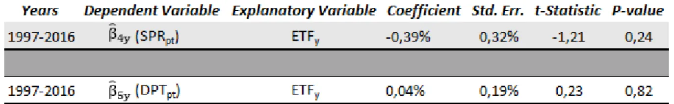
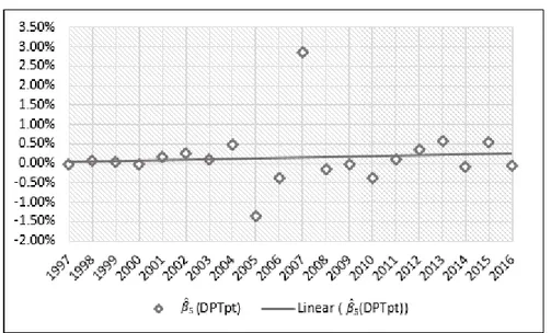
After calculating the ETF variable for the twenty years between 1997 and 2016, it was used as an explanatory variable when regressing against the estimated liquidity premium coefficients 𝛽̂4𝑦 and 𝛽̂5𝑦. The ETF variable was not tested against the liquidity variables SPR and DPT directly since it is only hypothesized in this thesis that ETFs affects the magnitude of the liquidity premium and not the spreads or the depths of stocks.

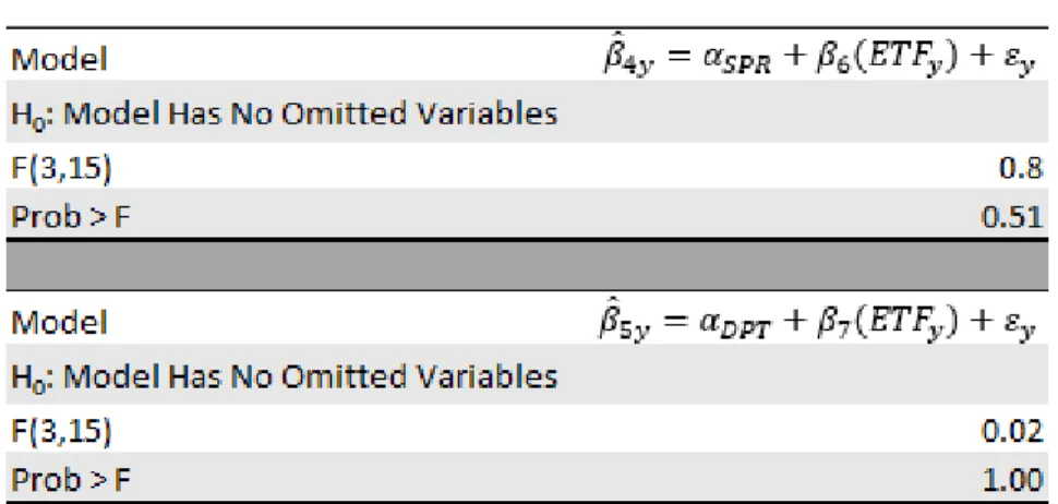
𝛽̂4𝑦= 𝛼𝑆𝑃𝑅+ 𝛽6(𝐸𝑇𝐹𝑦) + 𝜀𝑦 (8) 𝛽̂5𝑦= 𝛼𝐷𝑃𝑇+ 𝛽7(𝐸𝑇𝐹𝑦) + 𝜀𝑦 (9)

for y = 1,2,...,Y (Year)

Where:

𝛽̂4𝑦 was the previously estimated coefficient for the 𝑆𝑃𝑅𝑝𝑡 variable in year y. 𝛽̂5𝑦 was the previously estimated coefficient for the 𝐷𝑃𝑇𝑝𝑡 variable in year y.

𝛼𝑆𝑃𝑅 is the estimate of the mean value of the characteristic liquidity premium if 𝐸𝑇𝐹𝑦 = 0. 𝛼𝐷𝑃𝑇 is the estimate of the mean value of the systematic liquidity premium if 𝐸𝑇𝐹𝑦 = 0. 𝐸𝑇𝐹𝑦 was the ratio of United States equity which was allocated in ETF funds in year y. 𝜀𝑦 was the error term in year y.

Data Collection

Equations (6), (8) and (9) were used in regressions while equations (2), (3), (4), (5) and (7) were used in order to acquire the variables needed for those equations. The data needed in the equations was collected for the years between 1997 and 2016. There were two reasons for choosing this time-period. Firstly, there is limited recent research about the liquidity premium, providing an opportunity to contribute to the research field. Secondly, these years made it possible to incorporate capital inflow to the ETF market due to their inception in the early 1990s.

The tests in this study are performed on stocks included in the market index NASDAQ Composite. The stocks in the index have varying size and characteristics which enables a diversified sample. The reason for conducting the study on a market index with corporations from mainly the United States was because it is the world’s largest ETF market and because reliable data from the country is readily accessible.

All stock data was downloaded from Thomson Reuters Datastream. Because the data was originally collected by someone else and compiled into a database it was secondary data. The decision to use Datastream was based on its broad available time series data. Data was obtainable for each component

(26)

22

stock of the NASDAQ Composite index for the relevant time period from the database. Furthermore, the data output was presented in a pliable way which made it possible to work with the data efficiently. The data retrieved from Datastream was the market values (MV), market-to-book values (MTBV), prices of stocks adjusted for capital actions (P), daily high prices of stocks (PH), daily low prices of stocks (PL), turnover by value (VA), turnover by volume (VO) and volume weighted average price (WVAP).

The one-month risk-free rates and the excess market returns were obtained from Kenneth French’s website (French, 2018) and was hence secondary data. The risk-free rates obtained were the one-month United States Treasury bill rate.

The acquired data mentioned above was used to calculate the variables 𝑅𝑃𝑅𝐹𝑝𝑡, 𝑅𝑀𝑅𝐹𝑡, 𝑀𝑉𝑝𝑡, 𝐵𝑇𝑀𝑉𝑝𝑡, 𝑆𝑃𝑅𝑝𝑡 and 𝐷𝑃𝑇𝑝𝑡 used in equation (6). Further details on how the variables were calculated is stated in Appendix A.

There were three steps involved when removing stocks from the sample:

1. In the data output retrieved from Datastream, stocks which were listed in a later period or that had already been delisted were included. Because of the inclusion of stocks which were not listed in the corresponding time period, those entries had to manually be removed from the output.

2. Stocks with incomplete data observations were manually removed. This was done in order to assure a balanced panel.

3. Stocks which were considered severe outliers were removed due to the risk of having possible negative interference with results reflecting the nature of the stock market. Furthermore, the presence of severe outliers increases the risk of heteroscedasticity (Gujarati & Porter, 2009). Stocks with an observation above a 25% SPR value and stocks with an observation above a 500% DPT value were removed. To put these values in a relation, the 95% percentile of the SPR variable was 7.9% and the 95% percentile of the DPT variable was 10.2%. The five stocks that were removed in this process can be found in appendix B.

In Table 2 below, the descriptive statistics for the 210 stocks used as the sample is presented. All the included stocks can be found in appendix C.

(27)

23

Table 2: Descriptive Statistics Stocks

Note that RIRF has a minimum observed return in excess of -100%, this was possible because the calculations of the returns were done using logarithmic returns. Also note the high kurtosis in some of the variables. The high kurtosis is present due to deviant observations still being present in the data even after removing the most severe outliers.

The data for the capital allocated to ETFs was retrieved from ICI (2017). ICI had data for all the years in the relevant time period 1997-2016. The data for the total United States market equity value was retrieved from The World Bank (n.d.) and it covered the entire time period. Both of these datasets were secondary data in this study.

Portfolio Construction

Ten basis portfolios were constructed from the stock sample using a composite measure of both the characteristic and systematic liquidity variables. For each year, stocks were ranked based on their SPR multiplied by their DPT in January and the portfolios were then formed based on this measure. When testing the liquidity premium, portfolio formation is often done by using stocks’ liquidity ratios, for example by Amihud and Mendelson (1986a) and Eleswarapu (1997). The stocks with the highest value constituted portfolio 1 and the stocks with the lowest value constituted portfolio 10 for each year. The portfolios were constructed equally-weighted with 21 companies in each and were rebalanced annually. The creation of portfolios was done in order to decrease the high idiosyncratic volatility of individual stocks.

(28)

24

The kurtosis and skewness of the data has decreased at the expense of less observations. Even though more observations generally provide better results, the loss of observations does not critically impact the method since there are still 2400 observations for each variable.

Regression Method

The Fama-MacBeth regression approach is a common method to estimate the risk premium of different risk factors. It is also common to employ this method when investigating the liquidity premium. Authors which use the Fama-MacBeth approach when researching the premium includes Amihud and Mendelson (1986), Eleswarapu (1997), and Ben-Rephael et al. (2015) to name a few. Another option to test the relationship between variables and returns is to do a time-series regression with Fama-French return factors. When testing the liquidity premium in this thesis, the Fama-MacBeth approach was applied on equation (6) to test the liquidity risk factors SPR and DPT because it is a common approach when investigating risk factors.

To be able to draw conclusions of trends in the liquidity premium as well as for the existence of a premium for the whole period and sub-periods, 1-year regressions, 5-year regressions and a full 20-year regression was conducted. The 1-year regressions consisted of twelve periods, one for each month. With ten portfolios and twelve periods the 1-year regressions had 120 observations. These regressions were made in order to investigate the trend of the liquidity premium as well as a way to obtain the coefficients used to test how ETFs has affected the premium. It made it possible to investigate how the liquidity coefficients changed over time. Each of the 5-year regressions consisted of 600 observation. In total four 5-year regressions were made: 1997-2001, 2002-2006, 2007-2011 and 2012-2016. The full 20-year test period regression had 2400 observations and was made in order to see if any conclusions could be drawn by looking at the entire period.

When the 1-year coefficients for the liquidity variables were obtained from the Fama-MacBeth regression, the impact of ETFs could be tested. The coefficient results were used as dependent variables and the ETF variable as the explanatory variables. The tests were done using time-series regression because the data only had one dimension - time. The time-series regressions were made on equations (8) and (9).

Quality of the Method

Results from empirical studies are only useful if they are obtained by using a correct and unbiased process. When conducting research there is always a possibility of errors in the data or in the calculations. The data from Datastream and the other sources have been trusted to be correct due to their authoritativeness. The risk of being exposed to inaccuracies in the data has been mitigated by being critical and by verifying with additional sources. There is also the element of human error present when

(29)

25

handling and compiling data after it has been retrieved. By sticking to declared standards and being attentive in the procedure of creating the finalised spreadsheets the risk of human error has been minimized. Additionally, it is assumed that the models are correctly specified and that they include all the relevant variables. If any relevant variables would be omitted, the models would suffer from specification bias which could lead to autocorrelation and heteroscedasticity (Gujarati & Porter, 2009).

When working with data, biases may occur. Two common types of biases are “sample selection bias” and “survivorship bias”. Sample selection bias means that the sample which is tested does not represent the entire population (Heckman, 1979). A problem that can arise with this bias is how well the results corresponds to the entire population and the subjects which were excluded. The sample selection bias can hence impair the external validity of a test. Survivorship bias means excluding units which have not made it past some kind of barrier, this means that “failures” are excluded (Linnainmaa, 2013). This is a common bias in financial research since companies which have been delisted or has gone into bankruptcy are often excluded. Imagine that a researcher wants to test the average stock market return over a long time period, by excluding delisted stocks the researcher would typically receive overly optimistic results. In this thesis, both sample selection bias and survivorship bias may be present. Because of the removal of stocks with incomplete data, a certain type of stocks are excluded, the ones which lack data, typically stocks with extremely low liquidity. However, because the sample still includes stocks with a wide range of liquidity values, results can still be received on the relationship between returns and liquidity. Survivorship bias may also be present because only stocks which have data in all time periods are included. Because the cross-sectional regressions are performed on monthly returns, the effects of a possible survivorship bias are not as significant.

(30)

26

Empirical Results

In this chapter, the results from the diagnostics regressions for heteroscedasticity and autocorrelation as well as the results from the statistical measurements of the models (6), (8) and (9) are presented.

All of the statistical measures performed in this chapter are calculated in the software Stata. The output is assumed to have been correctly calculated inside the program. This also include the Boston College Archive package program “xtfmb” which is used to execute the Fama-MacBeth regression (Hoechle, n.d.). For each model, results are only considered to be statistically significant if they have a p-value below 0.05.

Robustness Tests

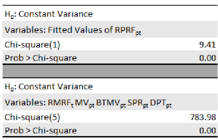
Because panel data is a combination of cross-sectional and time-series data, both autocorrelation and heteroscedasticity can exist in the data. If heteroscedasticity or autocorrelation is present it can impair the tests of significance. To ensure regressions without these drawbacks, diagnostics regressions were made to enquire whether they were present. To test for heteroscedasticity in the data, Breusch-Pagan tests (Breusch & Pagan, 1979) were carried out. The results of the tests are presented in Table 4 below.

Table 4: Breusch-Pagan Tests

The null hypothesis of homogeneity in the variance was rejected, both in the fitted values of the dependent variables as well as for the independent variables. It can be concluded that the data suffers from heteroscedasticity. Without proper actions, the standard errors would be biased when conducting the regressions. A consequence of biased errors is the risk of making wrong conclusions due to inaccuracies in the levels of significance.

To test for autocorrelation in the data, a Wooldridge test (Wooldridge, 2002) was performed. The result from the test is presented in Table 5.

(31)

27

Table 5: Wooldridge Test

The null hypothesis of no autocorrelation was rejected, meaning that autocorrelation is present. If unaccounted for, autocorrelation would bias the standard errors, which would impact the results.

To address the problems in the data, lags were included in the Fama-MacBeth regressions. The lag length was set to T-2, where T is the total number of months in the regression. T-2 is the maximum number of lags possible when executing the xtfmb package in Stata. By including the lags, Newey-West standard error estimates were obtained (Hoechle, n.d.). The Newey-West procedure is done in order to create a covariance matrix which accounts for heteroscedasticity and autocorrelation in the data which can make the estimates more accurate (Newey & West, 1987).

Liquidity Premium Results

To recap, the formula on which the liquidity premium regressions are based upon is:

𝑅𝑃𝑅𝐹𝑝𝑡= 𝛼𝑝𝑡+ 𝛽1(𝑅𝑀𝑅𝐹𝑡) + 𝛽2(𝑀𝑉𝑝𝑡) + 𝛽3(𝐵𝑇𝑀𝑉𝑝𝑡) + 𝛽4(𝑆𝑃𝑅𝑝𝑡) + 𝛽5(𝐷𝑃𝑇𝑝𝑡) + 𝜀𝑝𝑡 (6)

Since the focus of this study is the liquidity premium, the interesting empirical results are the sign, the magnitude and the significance of 𝛽4(𝑆𝑃𝑅𝑝𝑡) and 𝛽5(𝐷𝑃𝑇𝑝𝑡) which are proxies for the characteristic risk premium and the systematic risk premium. The full regression outputs are presented in appendices D-F. Only the liquidity premium coefficients are presented when we report the empirical results below in order to avoid deviating from the purpose of the thesis.

4.2.1 20-Year Results

The results for the entire 20-year period cross-sectional Fama-MacBeth regression is presented in Table 6. The table includes the coefficients of the SPR and DPT variables, along with the corresponding Newey-West standard errors and the resulting t-statistic.

(32)

28

Table 6: 20-Year Regression

*** Significant at 1% ** Significant at 5% * Significant at 10%

The regression result for the SPR variable show that there is a significant negative relationship between the spread and the returns of stocks. Given these results, a stock with a 1% higher spread than another stock would yield on average 0.49% lower monthly return. The DPT on the other hand, has a significant positive relationship with return, indicating that there is a positive systematic liquidity premium present. The result implies that a stock with a 1% higher DPT ratio than another stock return on average 0.15% better on a monthly basis.

4.2.2 5-Year Results

The output for the cross-sectional Fama-MacBeth regression for the four sub-periods are presented below in Table 7. The two tables present the results for the periods 1997-2001, 2002-2006, 2007-2011 and 2012-2016 for 𝑆𝑃𝑅𝑝𝑡 and 𝐷𝑃𝑇𝑝𝑡.

Table 7: 5-Year Regressions

*** Significant at 1% ** Significant at 5% * Significant at 10%