Effects of motion parallax in driving simulators

Effects of motion parallax in driving simulators

(1) Swedish National Road and Transport Research Institute, E-mail : {jonas.andersson.hultgren, bjorn.blissing,

jonas.jansson}@vti.se

Abstract – Motion parallax due to the driver’s head movement have been implemented and tested in VTI Driving Simulator III. An advanced camera-based system was used to track the head movements of the driver. The output from the tracking system was fed to the simulation software, which used low-pass filtering and a forward prediction algorithm to calculate an offset. The offset was then used by the graphics software to display the correct image to the driver.

The effects of driving with motion parallax in the simulator were also observed by an initial study. During the experiment, the subjects caught up with several slower vehicles which forced the driver to make an overtaking maneuver. Oncoming traffic forced the subject to search for a suitable gap for overtaking. The study also included a speed perception test. The results from the study showed no difference in lateral positioning when running behind a slower vehicle nor in speed perception with and without motion parallax.

Key words: driving simulator, motion parallax, depth cues, distance perception, speed perception

Introduction

Motion parallax has been shown to be an important source of depth information, both when the observer makes lateral movement relative to an object as well as when an object moves relative to a stationary observer [Rog1]. In modern driving simulators most relevant visual depth cues are available, such as relative size, occlusion and shadows. However, cues like motion parallax due to the driver’s head movement and stereoscopic view are often missing because of the additional cost and complexity of such systems [Kem1]. The absence of such visual cues might be a reason why different driving behaviour is observed in driving simulators compared to real-life driving. It has been suggested that motion parallax arising from driver head movement might be necessary for improved depth perception in driving simulators [Kem1].

The aim of the project was to implement motion parallax due to driver’s head movement in the VTI simulation system. A small study was performed, mainly focusing on distance perception. This was done to evaluate if the additional depth information affects driving behaviour in a driving simulator.

It is commonly known that distances are underestimated in virtual environments and that people tend to drive faster in simulators than in real life [Bau1][Boe1]. Because of this a speed perception test was also included in the study.

Methods

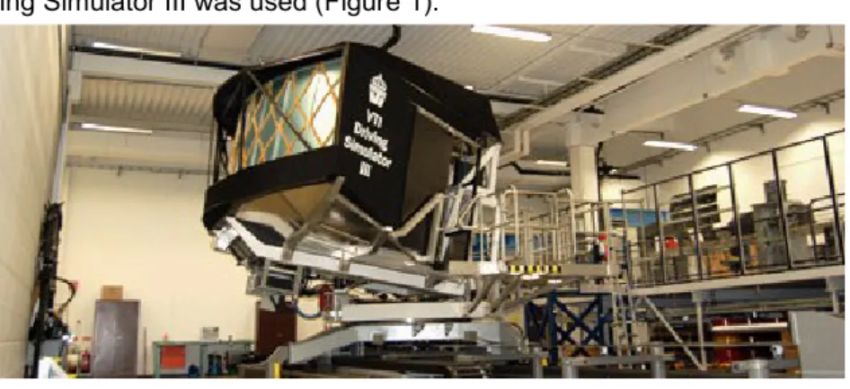
In this project VTI Driving Simulator III was used (Figure 1).

Figure 1. VTI Driving Simulator III

The simulator features a high-performance linear motion system for simulation of realistic lateral forces experienced when driving [Nor1]. The motion system also includes roll and pitch movements of the whole simulator

platform, as well as a vibration table for simulating road roughness and bumps. The vibration table is located under the passenger car cabin installed in the simulator, and provides vibration movement relative to the projection screen. The driving environment is presented to the driver on the projection screen by three projectors, each with a resolution of 1280x1024 pixels, providing 120 degrees field of view, as well as in three rear view mirrors. Image rendering is performed in 60 Hz. The driver is located three meters in front of the projection screen.

Head movement tracking equipment

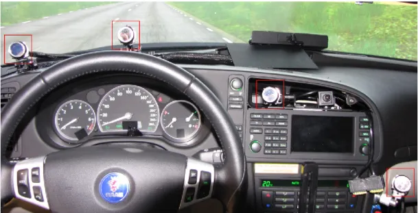
An advanced camera-based tracking system was used for measuring the driver’s head position while driving [And1]. The tracking system is capable of measuring, among other things, the driver’s head position, head rotation and gaze direction in three dimensions. For this project a four-camera tracking system was used. The cameras were located about 80 centimetres from the driver’s head (depending on seat adjustments), allowing maximum lateral head movements of 15 to 20 centimetres in each direction from the centre point without losing tracking. The camera placement in the simulator cabin can be seen in Figure 2. The tracking system provided new data at approximately 100 Hz.

Figure 2. Camera placement in simulator cabin. Cameras highlighted by red markers.

Implementation of motion parallax algorithm

The basic flow of the algorithm can be seen in Figure 3. The simulation software reads the output from the head tracking system, filters the signal and then calculates a new output position using a forward prediction algorithm. The output is then sent to the graphics software which changes the viewpoint from which the image is rendered according to this data. Special consideration had to be made when tracking was lost and later regained. The different parts of the algorithm are explained in more detail below.

Figure 3. The basic flow of the motion parallax algorithm.

When motion parallax is activated during simulation, the current head position of the driver is used as origin for future calculations, as the driver most often is not located in the origin of the tracking system’s coordinate system. In the first step of the algorithm, the input from the head tracking system is passed through a low pass filter before being fed to the forward prediction algorithm. Each dimension is filtered separately, with potentially different cut-off

Read input from tracking system

Low pass filtering

Forward prediction algorithm

frequencies, to accommodate the different needs for filtering. This would however introduce more time delay into the system, so it was important to keep the filtering to a minimum, particularly for lateral head movements which are most common for a driver. The rear view mirrors were particularly susceptible to noise due to their position close to the driver and further low pass filtering was added for them specifically.

In the second step, a forward prediction algorithm is used to compensate for the time delays in the simulation system and make the motion parallax algorithm responsive on the driver’s head movements. For this implementation Double Exponential Smoothing-based prediction (DESP) is used [LaV1].

Special considerations had to be made when tracking was lost, which for instance could happen if the driver left the cameras’ detection zone, or if the face was obstructed by an object. As it is difficult to anticipate how and where the driver moves when tracking is lost, and to avoid that the visual presentation “drifts away”, the motion parallax algorithm stops producing new outputs and stays in the last position until tracking is resumed. When tracking is resumed, a smooth transition is made from the old position to the new position to avoid jerks in the visual presentation.

The motion parallax algorithm is based on the driver’s head position only. In the planned scenarios the head rotations were expected to be minimal and thus head rotation was not taken into consideration. The algorithm produces output in all three dimensions.

Calculating the parallax effect on the screen

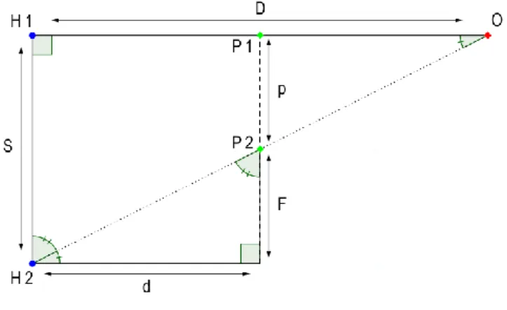
Given that the observer moves in parallel with the screen and have gaze direction perpendicular to the screen surface, triangle similarity can be used to calculate the amount of displacement caused by the parallax effect (see Figure 4 and Table 1).

Figure 4. Geometry for calculation of parallax effect.

Table 1. Symbols for calculation of parallax effect.

Symbol Description

O Object in simulator world D Distance to the object (H1, O) d Distance to the screen

S Distance between observer positions (H1, H2) p Distance between the projected object (P1, P2) Triangle similarity can be used to describe the relationship between the distances:

(1)

From Figure 4 the following correlation can be derived:

(2)

Inserting Eq. 2 into Eq. 1 produces:

Solving Eq. 3 for p:

(4)

Considering an object at infinite distance:

( ) (5)

Eq. 5 shows that an object at infinite distance will be moved in sync with the observer, i.e. the object will be perceived as standing still relative to the observer.

Objects closer than infinity will not move in sync with the observer which will result in the parallax effect. This effect is the difference between the movement of the projected object (P1, P2) and distance the observer has travelled (H1, H2):

(6)

Calculating the limit of the parallax effect

There is a limit on how far humans can perceive the parallax effect. This limit depends on two factors; the visual acuity of the eye and the motion of the observer. Visual acuity is defined as ⁄ , where A is the response in line pair/arc-minute. The human eye has a visual acuity of 1.7 [Art1][Hec1], which corresponds to 0.59 arc-minute/line pair.

The simulator screen used in the study has a resolution of 4.2 arc-minute/line pair [VTI1], which limits the effect further. The simulator cabin also limits the motion of the observer. In our study we recorded an average range of lateral motion of the observer of 0.1 meter.

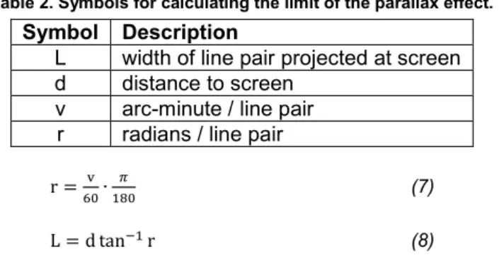
The limit of the parallax effect can be defined as the distance at which an object remains at the same position on the screen relative to the observer’s position. When the parallax effect results in a projected movement less than the projected line pair width, the object is perceived as being at infinite distance from a parallax point of view. The projected line pair width can be calculated by Eq. 7 and Eq. 8 below. Symbols descriptions are listed in Table 2.

Table 2. Symbols for calculating the limit of the parallax effect.

Symbol Description

L width of line pair projected at screen d distance to screen

v arc-minute / line pair r radians / line pair

(7)

₍₈₎

Eq. 6 and Eq. 8 can be used to calculate the distance where the parallax movement is equal to the projected line pair width, i.e. the limit of the parallax effect.

(9)

Inserting the values from the simulator study limits the parallax effect to roughly 80 meters. If projectors were available that could reach the same resolution as the human eye, the driver should be able to see the parallax effect of objects almost 600 meters away.

Evaluation study

Finally, a small study was conducted to evaluate the system in the simulator. 22 participants (twelve men, ten women) were recruited for the study and they were between 22 and 63 years old (average 43.4). Each subject drove the same scenario twice, once with motion parallax enabled and once disabled. The order was fairly balanced (nine enabled first and 13 disabled first) between the participants. They were not made aware that motion parallax would be available.

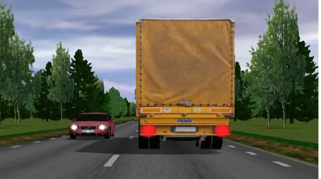
The driving scenario in the study consisted of three overtaking situations of slower vehicles including a car, a bus and a truck (Figure 5) on a 24 kilometer long single-track rural road. The road had a posted speed limit of 90 kilometers per hour, while the slower vehicles traveled at a speed of 70 kilometers per hour. In each situation, oncoming cars forced the participant to search for a suitable gap to safely complete the overtaking maneuver. The gaps between the oncoming cars increased for each vehicle and were the same for all three situations. Eight gap sizes were used; 100, 150, 200, 300, 300, 400, 400 and 600 meters. After each situation the subjects were asked to judge how difficult it was to find a suitable gap for overtaking the preceding vehicle. The order of the overtaking situations was balanced between the subjects and the same subject never had the same order in both parts. There was no traffic on the road between the different overtaking situations. Participants were encouraged to overtake slower traffic.

In addition to the overtaking situations, a speed perception test was included at the end of each run. The speed limit on the road was lowered first to 70 kilometers per hour, and then to 50 kilometers per hour and the participants were asked to stay as close to the speed limit as possible. Before reaching the first speed limit change, the speedometer and tachometer were turned off. The participants were informed before the experiment that this would happen and also reminded after the final overtaking situation. Also, the road marks were changed to solid white lines to eliminate the road marks as a speed perception cue. The length of the 70-zone was 750 meters, while the 50-zone was 500 meters. After this part of the experiment, the subjects were asked to judge how difficult it was to estimate their own velocity.

Figure 5: Overtaking situation involving a truck.

Results and discussion

The primary measurement in this study was the lateral positioning of the own vehicle when searching for a suitable gap for overtaking. This measurement was calculated by taking the average lateral position from the point in time when the driver got within 50 meters of the vehicle in front, until the driver initiated the overtaking maneuver. Each kind of overtaking situation (car, bus, truck) was analyzed on its own, as well as bus and truck combined since they obscured the driver’s view equally. No significant differences driving with and without motion parallax was found in neither case.

Secondly, the raw data from the head tracking system was analyzed to find differences in the subjects’ head movements with and without motion parallax. It was observed that the subjects did move their head when running behind preceding vehicle trying to get a better view of the oncoming traffic. The same behaviour was observed regardless of the use of motion parallax.

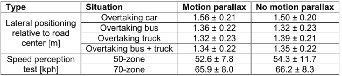
Finally, the data from the speed perception test was analyzed, including average velocity and lateral positioning of the vehicle. The measurements were calculated over the whole 70- and 50-zones respectively, but no significant differences were found. The measurements from the study are shown in Table 3.

For the subjective measurements collected through questionnaires, we could not see any trends regarding neither the difficulty to find a suitable gap for overtaking nor for the self-speed perception.

Likewise, no increase in simulator sickness in relation to the use of motion parallax could be observed. This was also based on subjective measurements from the subjects through questionnaires. There were no discontinued test drives due to simulator sickness. Also, most subjects failed to notice any difference between the two runs.

Table 3. Mean value and standard deviation for study measurements.

Type Situation Motion parallax No motion parallax

Lateral positioning relative to road center [m] Overtaking car 1.56 ± 0.21 1.50 ± 0.20 Overtaking bus 1.36 ± 0.22 1.32 ± 0.23 Overtaking truck 1.32 ± 0.23 1.39 ± 0.21 Overtaking bus + truck 1.34 ± 0.22 1.35 ± 0.22 Speed perception

test [kph]

50-zone 52.6 ± 7.8 54.3 ± 11.7

70-zone 65.9 ± 8.0 66.2 ± 8.3

In conclusion, we do not see any significant effects on the driving behaviour, i.e. vehicle lateral lane position, speed perception and driver head movements, in this study.

We have considered why we couldn’t see any significant effects and have the following theories. One theory is that motion parallax due to head motion is not used by drivers to estimate distances in the types of scenarios included in the study. An interesting comparison would be to perform the alignment and bisection tasks used in [Bau1] where subjects are required to position their own car at predefined positions relative to other vehicles.

Another theory could be that the image resolution in the simulator is too low to give a realistic parallax effect. Inter-scenario learning effects during the experiment could also be a potential error source. Since the subjects experience the same situations several times, their driving behaviour might change over the course of the experiment, e.g. they might be keener on overtaking the preceding vehicle in the first situation while taking a more cautious approach in subsequent situations knowing that they won’t be able to overtake right away.

References

[And1] Andersson Hultgren, J. “Methods for improved visual perception in driving simulators”. Master Thesis,

Linköping University, Linköping. 2011.

[Art1] Arthur, K. “Die Abhängigkeit der Sehschärfe von der Beleuchtungsintensität”. Berlin: Akad Wissensch Berlin,

1897.

[Bau1] Baumberger, B., Flückinger, M., Paquette, M., Bergeron, J., Delorme, A.”Perception of relative distance in a

driving simulator”. Japanese Psychological Research, 2005, 47(3), pp. 230-237.

[Boe1] Boer, E. R., Yamamura, T., Kuge, N., & Girshick, A. “Experiencing the Same Road Twice: A Driver

Centered Comparison between Simulation and Reality”. Driving Simulation Conference, 2000.

[Hec1] Hecht, S. “The Retinal Processes Concerned with Visual Acuity and Color Vision”. Howe Laboratory of

Ophthalmology, Harvard Medical School, 1931, Bulletin No. 4. Cambridge: Harvard University Press.

[Kem1] Kemeny, A., & Panerai, F. “Evaluating perception in driving simulation experiments”. Trends in Cognitive

Sciences, 2003, 7(1), pp. 31-37.

[LaV1] LaViola Jr., J. “Double Exponential Smoothing: An Alternative to Kalman Filter-Based Predictive Tracking”.

Eurographics Workshop on Virtual Environments, 2003, pp. 199-206.

[Nor1] Nordmark, S., Jansson, H., Palmkvist, G., & Sehammar, H. ”The new VTI Driving Simulator - Multi Purpose

Moving Base with High Performance Linear Motion”. DSC Europe, Paris, 2004.

[Rog1] Rogers, S., Rogers, B. J. “Visual and nonvisual information disambiguate surfaces specified by motion

parallax”. Perception & Psychophysics, 1992, 52(4), pp. 446-452.

[VTI1] VTI's driving simulators. Retrieved from