Speeding up matrix computation kernels by sharing vector coprocessor among multiple cores on chip

(1)

Postal address: Visiting address: Telephone:

Speeding up matrix computation kernels by

sharing vector coprocessor among multiple

cores on chip

Christopher Dahlberg

EXAM WORK 2011

(2)

(3)

Postal address: Visiting address: Telephone:

This thesis work is performed at Jönköping University, School of Engineering, within the subject area Electrical Engineering. The work is part of the two year master’s degree programme with the specialization in Embedded Systems. The author takes full responsibility for opinions, conclusions and findings presented. The research for this exam work was carried out from March to May 2011 at the CAPPL (Computer Architecture and Parallel

Processing L:aboratory) Laboratory of the New Jersey Institute of Technology (USA) while the author was on leave from the School of Engineering in

Jönköping.

Supervisors: Spiridon Florin Beldianu, Shashi Kumar and Sotirios Ziavras Examiner: Shashi Kumar

Scope: 30 credits (ECTS) Date: 29/07/2012

(4)

Abstract

Abstract

Today’s computer systems develop towards less energy consumption while keeping high performance. These are contradictory requirement and pose a great challenge. A good example of an application were this is used is the smartphone. The constraints are on long battery time while getting high performance required by future 2D/3D applications. A solution to this is heterogeneous systems that have components that are specialized in different tasks and can execute them fast with low energy consumption. These could be specialized i.e. encoding/decoding, encryption/decryption, image processing or communication.

At the apartment of Computer Architecture and Parallel Processing Laboratory (CAPPL) at New Jersey Institute of Technology (NJIT) a vector co-processor has been developed. The Vector co-processor has the unusual feature of being able to receive instructions from multiple hosts (scalar cores). In addition to this a test system with a couple of scalar processors using the vector processor has been developed. This thesis describes this processor and its test system. It also shows the development of math applications involving matrix operations. This results in the conclusions of the vector co-processing saving substantial amount of energy while speeding up the execution of the applications.

In addition to this the thesis will describe an extension of the vector co-processor design that makes it possible to monitor the throughput of instructions and data in the processor.

Keywords

 Coprocessor  Speeding-up  Accelerator  Power efficiency  Shared resources  Vector processor  Multi-core on chip

(5)

Contents

1 Introduction ... 1

1.1 BACKGROUND ... 1

1.2 NEED FOR HIGH PERFORMANCE COMPUTING AND PARALLEL COMPUTING ... 1

1.3 GOALS AND SCOPE ... 2

1.4 THESIS OUTLINE ... 2

2 Theoretical background: Parallel Architectures and Their

Programming ... 4

2.1 PARALLEL ARCHITECTURES ... 4

2.1.1 Pipeline computers/MISD ... 4

2.1.2 SIMD ... 4

2.1.3 MIMD ... 5

2.2 MULTICORE AND MULTIPROCESSORS (MULTIPROCESSORS (PARALLEL AND MULTI-CORE ARCHITECTURES)) ... 5

2.3 COPROCESSORS ... 6

2.4 VECTOR PROCESSORS ... 6

2.4.1 Vector lanes ... 7

2.4.2 Vector stride ... 8

2.5 ENERGY CONSUMPTION IN ELECTRONIC DEVICES ... 9

2.5.1 Dynamic power ... 10

2.5.2 Static power ... 10

2.5.3 Solutions for low energy consumption ... 10

3 Vector Coprocessor Architecture ... 11

3.1 TEST SYSTEM ... 11

3.2 VECTOR COPROCESSOR ... 12

3.2.1 Vector lanes ... 14

3.2.2 Scheduling ... 16

3.2.3 Instructions ... 18

4 Method and Development tools ... 22

4.1 HARDWARE/SOFTWARE DEVELOPMENT ... 22

4.2 PROTOTYPING VECTOR PROCESSOR ARCHITECTURE ... 23

4.3 SYSTEM SIMULATION AND ANALYSIS ... 23

5 Application Development and Performance Evaluation .... 25

5.1 APPLICATION DEVELOPMENT PROCESS ... 25

5.2 MATRIX-MATRIX MULTIPLICATION ... 26

5.2.1 Mapping of application on architecture ... 27

5.2.2 Pseudo code of mapped application ... 32

5.2.3 Performance evaluation of the application ... 33

5.3 LU-DECOMPOSITION ... 34

5.4 SPARSE MATRIX-VECTOR MULTIPLICATION ... 39

6 Extension of the Architecture ... 43

6.1 MOTIVATION FOR EXTENSION ... 43

(6)

Contents

6.3 THROUGHPUT MEASURING BLOCK DESIGN ... 43

6.4 TEST AND PERFORMANCE ... 45

7 Discussion and conclusions ... 46

7.1 DISCUSSION OF METHOD ... 46 7.2 CONCLUSIONS ... 46 7.3 FUTURE WORK ... 47

8 References ... 48

9 Appendices ... 50

9.1 APPENDIX I ... 51 9.2 APPENDIX II ... 52

(7)

Table of figures

Table of figures

FIGURE 1 – OVERVIEW OF THE TEST SYSTEM. 2

FIGURE 2 - TYPICAL VECTOR PROCESSOR ARCHITECTURE OF THE VECTOR-REGISTER

TYPE. [3]. 7

FIGURE 3 - ILLUSTRATING A NORMAL SEQUENTIAL ADDITION AND A PARALLEL

ADDITION BETWEEN THE ELEMENTS OF A VECTOR A AND B [3]. 8

FIGURE 4 – TWO 4X4 MEMORIES WITH VECTORS STORED IN DIFFERENT WAYS. 9

FIGURE 5 – THE ARCHITECTURE OF THE TEST SYSTEM. 11

FIGURE 6 - OVERVIEW OF THE WHOLE SYSTEM SHOWING A SETUP WITH TWO CPUS

CONNECTED TO THE HIGHLIGHTED VP. 12

FIGURE 7 – DETAILED ARCHITECTURE OF THE VP. 14

FIGURE 8 – A VECTOR LANE IN VP. 16

FIGURE 9 – FLOWCHART DESCRIBING AN APPLICATION DEVELOPMENT AND

EXECUTION PROCESS. 26

FIGURE 10 – ILLUSTRATING HOW A LARGE MATRIX-MULTIPLICATION PROBLEM IS

SPLIT INTO SECTIONS. 28

FIGURE 11 – SHOWING THE CALCULATION OF THE FIRST SECTOR IN THE MATRIX 29 FIGURE 12 - SHOWING A COMPARISON BETWEEN A SEQUENTIAL MATRIX

MULTIPLICATION AND A PARALLEL MATRIX MULTIPLICATION. IT TAKES 45 SCALAR INSTRUCTIONS TO DO THIS MATRIX MULTIPLICATION, BUT ONLY 18 VECTOR INSTRUCTIONS. THE ADVANTAGE OF A VP IS OBVIOUS AND WOULD BE EVEN MORE OBVIOUS WITH A LARGER VECTOR SIZE, E.G. EIGHT, WHICH IS THE

NUMBER OF VECTOR LANES ON THE VP USED IN THIS THESIS. 31

FIGURE 13 – TIMELINE DESCRIBING THE EXECUTION OF THE SEQUENTIAL AND THE PARALLEL EXECUTION OF THE PREVIOUSLY PRESENTED EXAMPLE, ASSUMING ONE CORE USING THE VP WITH CTS. THE NUMBERS WITHIN THE BLOCKS SAYS

WHICH ELEMENT(S) IS/ARE EXECUTED. 32

FIGURE 14 - PSEUDO CODE OF MATRIC MULTIPLICATION 32

FIGURE 15 - GRAPHICAL ILLUSTRATION OF THE RECURSIVE ALGORITHM OF LU

DECOMPOSITION 35

FIGURE 16 – PSEUDO-CODE DESCRIBING THE IMPLEMENTATION OF THE FIRST

VERSION. BOLD TEXT INDICATES OPERATIONS EXECUTED BY THE VECTOR

PROCESSOR. 37

FIGURE 17 - PSEUDO-CODE DESCRIBING THE IMPLEMENTATION OF THE SECOND

VERSION. BOLD TEXT INDICATES OPERATIONS EXECUTED BY THE VECTOR

PROCESSOR. 37

FIGURE 18 – SHOWING A MATRIX ILLUSTRATED IN A TYPICAL MATHEMATICAL

NOTATION TO THE LEFT AND ACCORDING TO CSR ON THE RIGHT. 39

FIGURE 19 – CODE FOR MULTIPLICATION-PART OF THE SPARSE-MATRIX-MULTIPLICATIONS. BOLD CODE TEXT CORRESPONDING TO

VECTOR-INSTRUCTIONS. 41

FIGURE 20 – CODE OF THE MIXED VERSION, SIMPLIFIED PRESENTATION BECAUSE IT IS

A MIX OF THE PREVIOUS TWO IMPLEMENTATIONS. 41

FIGURE 21 – BLOCK ILLUSTRATING THE BLOCK DESIGNED IN VHDL TO MEASURE THE

(8)

Abbreviations

Abbreviations

SIMD Single Instruction, Multiple Data streams MISD Multiple Instruction, Single Data stream MIMD Multiple Instruction, Multiple Data streams FTS Fine-grain Temporal Sharing

CTS Coarse-grain Temporal Sharing VLS Vector Lane Sharing

FIFO First In, First Out ALU Arithmetic Logic Unit FPU Floating-Point Unit CPU Central Processing Unit VP Vector Processor

VL Vector Length

CSR Compressed Sparse Row FSB Front Side Bus

(9)

Introduction

1 Introduction

1.1 Background

This project was done at the Electrical and Computer engineering at New Jersey Institute of Technology (NJIT) in Newark New Jersey. The thesis work was part of the research conducted by Professor Sotirios Ziavras and PhD student Spiridon Florin Beldianu at Computer Architecture and Parallel Processing Laboratory (CAPPL). The research has resulted in a Vector co-processor with the unique behavior of being shared between several hosts. There was a need for

benchmarking this architecture and that’s where this thesis filled its purpose. Mathematical applications running on hosts using the Vector co-processor had to be written. By running these applications with different setups an evaluation of the test system could be done. In addition to that prof. Ziavras and mr. Beldianu gave me the opportunity to prototype extra functionality to the architecture.

To run the applications a test system was already developed and implemented in VHDL code. This was then used for simulation with the applications that were designed and the extension of the processor.

1.2 Need for High performance computing and Parallel

computing

Traditionally increase of performance of computer systems has been achieved by increasing the clock frequency. Due to difficulties in increasing the clock

frequency further new directions are being explored. For the last years focus has been on introducing more processor cores in the computer systems. This has resulted in continuous increase of performance. The next generation of multi-core systems has a different approach, called heterogeneous system. These systems combine computing units with different specialties. In this way, a lot of special functionality can be put on one chip. The result is a multifunctional system with low energy consumption per atomic operation and high application throughput. Energy consumption is a big topic today. For example, smartphones combine high performance with batteries as power source.

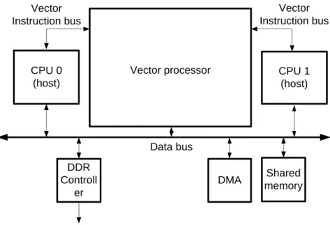
At NJIT, a special hardware unit for that purpose has been design. An experimental system including this special unit, a vector processor, has been designed. Figure 1 gives an overview of the architecture of the test system. The test system contains of a Vector Processor (VP) which can receive vector

instructions from multiple hosts/cores. In the test system there are two hosts that will run applications that will use the VP for vector intensive computation. The VP will then mix the instructions according to different scheduling schemes and do the vector operations according to the vector instructions [1] [2].

(10)

Introduction CPU 1 (host) Data bus CPU 0 (host) DMA DDR Controll er Vector Instruction bus Vector Instruction bus Shared memory Vector processor

Figure 1 – Overview of the test system.

1.3 Goals and Scope

There are two goals for this thesis:

The first goal of the thesis is to implement a number of applications for the test system that will do mathematical operations with the help of the vector processor. Mathematical methods chosen suggested by the developers of the test system were LU decomposition (also called LU factorization), Matrix-Matrix

multiplication and sparse matrix-vector multiplication. The design language demanded for the applications is C. The coding and the design is the practical job for this.

The second goal is to add profiling capability of the Vector Processor that is a feature that monitors hardware performance with an instruction counter. This could for example be used in future scheduling schemes were the host access to the Vector processor could be prioritized according to previous usage of the Vector processor.

1.4 Thesis Outline

Chapter 2 contains background material to give the reader more understanding about the theory behind this thesis. It explains parallel computing and vector processing. It also presents vector processors and in particular the VIRAM processor that is an example of a vector processor.

(11)

Introduction

In Chapter 6 the second practical task of the thesis is explained. It describes about the extension that were made to the architecture.

Chapter 7 will conclude the report with a discussion about the work that have been done and also about possibility of future work in the area of this thesis.

(12)

Theoretical background: Parallel Architectures and Their Programming

2 Theoretical background: Parallel

Architectures and Their Programming

2.1 Parallel architectures

Parallel computer architectures can be divided in different types. According to Flynn’s taxonomy there are in general four types: Single Instruction Single Data (SISD), Single Instruction Multiple Data (SIMD), Multiple Instructions Multiple Data (MIMD), Pipeline computers or Multiple Instructions Single Data (MISD) [3] [4].

2.1.1 Pipeline computers/MISD

Most processors today are pipelined in the context that they divide the

instructions into several stages so that several instructions can be in progress at the same time. This will increase the throughput and the utilization of the processor. A downside with pipelines is that they increase the latency, the time from when an instruction is started until it is finished. Another downside is when the code got a lot of branches, meaning conditionals leading to different execution of instructions. If an instruction is already in the pipeline and a previous

instruction just finished its last stage which affects a conditional before the first mentioned instruction. The instruction that came after the one affecting the conditional might be useful because another branch should be executed. In that the case the pipeline has to be “flushed” and the process of filling up the pipeline will restart. The main advantage of a pipeline computer is when executing a sequential stream of instructions. Then the throughput is close to or equal to one instruction per clock cycle for single issue processors [5].

MISD implies different operations are being carried out on one data. There are no good examples of these systems. According to some descriptions a Pipeline

computer can be considered as a MISD. With that assumption also Systolic arrays could be included in this category. A Systolic array is basically a two or multi-dimensional pipeline system [3].

2.1.2 SIMD

SIMD or sometimes called Array computers means that there are several

processing elements (PEs). These are executing operations in parallel. There is one controller that is decoding the instruction and all the PEs are processing the same

(13)

Theoretical background: Parallel Architectures and Their Programming 2.1.3 MIMD

MIMD means that processors are doing independent computations on independent data in parallel. There are a couple of variants of this type of architecture. The main difference between them are if they have shared memory or distributed memory (each processor have full control over its own memory or memory area). In the shared memory case there have to be some kind of

arbitrator or controller which distributes access time for the processors [10].

2.2 Multicore and Multiprocessors (Multiprocessors

(Parallel and multi-core architectures))

A multicore and multiprocessor are processors of the type MIMD. The difference between multicore and multiprocessor is that the multicore processors are on the same die and are usually more tightly connected when it comes to sharing

resources when it comes to Front Side Bus (FSB), memory and cache.

Multiprocessors usually don’t share die but will usually interact with each other in one way or another.

The problem that occurs when using multiple cores is the demands it put on the programmer. To make use of the systems performance there has to be code that makes use of it. The code must have parts that can be run in parallel. The

minimum is then that they at least run one thread per core. Some architectures allow many threads per core. The speedup using multiple cores can be calculated by using the formula derived from Amdahl’s law. It is presented by equation (1), where is the fraction of the parallel code that can be ran on all the cores in parallel.

(1) It is not unusual that the different CPU need to communicate with each other. There are a couple of ways for the different CPUs to communicate. A common way is by using messages. One CPU will send a message to another CPU using some kind of interconnection infrastructure like a bus or Network on Chip (NoC). Another way is by using a shared memory and store data which both CPUs can access. In this way a CPU that is making calculations that another CPU is dependent on can store them at location in the shared memory, which have been agreed on. These two kinds of communications can of course be mixed so that some communications is done by message passing and some by shared memory [3].

(14)

2.3 Coprocessors

A coprocessor is a processor that has the purpose to assist a CPU (Central Processing Unit). A coprocessor is sometimes called an accelerator. It has commonly a specialization, and gives therefore the CPU an extra feature or speedup. The specializations could for example be: bit based, integer and floating point arithmetic, vector arithmetic, graphics or encryption. A coprocessor cannot be the main unit and is therefore in need of a host for controlling it in some way. Some coprocessors can’t fetch instructions on its own, they then need instructions sent to it by the host. An example of a coprocessor is a GPU (Graphics

Processing Unit). Basically all PCs have a GPU. It is a coprocessor that will do graphics calculations for the CPU. This is used for gaming (3D processing), photo editing (Image processing) and Video (Decoding) etc.

2.4 Vector processors

A vector processor is a processor where one instruction can represent tens or hundreds of operations. Therefore, the area, time and energy overheads associated with fetching and decoding of SIMD instructions is a lot smaller in vector

processor than in a scalar processor. To give a comparison between a scalar processor and a vector processor consider an addition between two vectors of ten numbers to produce a new vector of ten numbers. In a scalar processor it could look something like this:

1 execute this loop 10 times 2

3 fetch the next element of first vector 4 fetch the next element of second vector 5 add them

6 put the results in the next element of the third vector 7 end loop

But when using a vector processor this could look like this:

1 read the vector instruction and decode it 2 fetch 10 numbers of first vector

3 fetch 10 numbers of second vector 4 add corresponding elements

5 put the results back in memory

An advantage with this is also that when using a vector instruction like this is that we ensure that the ten numbers have no data dependency and therefore the checking for data hazards between elements is unnecessary.

(15)

 Vector registers: Registers containing data in form of a vector. This is the data that is going to be processed.

 Vector functional units: Represents the different operations/functions the vector processor can do on data.

 Vector load/store unit: Handles transfers between main memory and vector registers.

 A controller that handles the correct functionality of the VP [11].

Figure 2 - Typical vector processor architecture of the vector-register type [3]. 2.4.1 Vector lanes

What gives the vector processor its parallel features are its vector lanes. The vector lanes contain computing elements which do calculation in parallel to other lanes. In Figure 3 (a) is an example of a single lane and in Figure 3 (b) an example of multiple lanes. The figure shows the execution of an addition between the elements of a vector A and a vector B. The example show how the addition is queued in different setups. In the example with only one lane can we see that all the elements are queued, while in the four lane example the elements are

(16)

Figure 3 - Illustrating a normal sequential addition and a parallel addition between the elements of a vector A and B [3].

2.4.2 Vector stride

Vector stride address the problem when adjacent elements in a vector are not stored with sequential positions in a memory. The Stride is the distance between the elements in the memory. Figure 4 shows the storage of three different 4-element vectors. They all are stored in 4x4 memories, (a) shows the memory address of the different positions in the memories. In (b) Vector A is stored with its adjacent elements sequentially while in (c) vector B is stored as a column vector. The stride in this case would be 4 while the “jump” between the elements is an address difference of 4. In (d) a vector C is stored as a diagonal vector, with a stride of 5.

(17)

1 2 3 4 A[0] A[1] A[2] A[3]

5 6 7 8 9 10 11 12 13 14 15 16 (a) (b) B[0] C[0] B[1] C[1] B[2] C[2] B[4] C[3] (c) (d)

Figure 4 – Two 4x4 memories with vectors stored in different ways. This is useful if a vector operation has to be done between a row vector and a column vector. Vector operations modified for stride are common variant of “normal” vector operations in vector processor instruction sets.

2.5 Energy consumption in electronic devices

The difference in energy consumption between different devices can vary a lot. In embedded system in general and mobile embedded system in particular low energy consumption is fundamental. This is obviously because many of them are battery powered. But lower energy consumption also means that less heat is generated, which also is important for many embedded system, especially mobile devices. The downside is that lower energy consumption generally means lower computation capacity. While focus for manufacturers of desktop computers and other stationary devices has been high performance the energy consumptions has risen for every generation. On the other hand, the classic mobile devices have had very low energy consumption, but also lesser performance. With the rise of laptops and smartphones these two worlds have to meet, high performance and low energy consumption at the same time. That is a difficult situation. One possible solution might be SIMD architectures.

In general energy consumption is divided into two different types, static and dynamic energy consumption.

(18)

Theoretical background: Parallel Architectures and Their Programming 2.5.1 Dynamic power

The dynamic energy consumption comes from when unwanted capacitances (parasitic capacitances) in electronic components charges and discharges. When Integrated circuit (IC) changes its state voltages these capacitances change and energy is emitted in the form of heat. This heat is unwanted and often has to be removed with the help of heat sinks and fans. The capacitances can be both intentional and unintentional. Intentional capacitances could be capacitances between gate-channel in a transistor. Unintentional is for example capacitances that occur between conductors. As long as switching is done (when the

components are clocked) there will be an dynamic power consumption 2.5.2 Static power

Static energy consumption comes from leakage current from transistors. Big efforts has been put into lowering the size of transistors, this has resulted in lowered dynamic power consumption. This means that the static power

consumption has become a greater portion of the total energy consumption in modern computer systems. In many of today’s high performance computers the power has increased dramatically and sometimes dominates the total power consumption [12].

2.5.3 Solutions for low energy consumption

So basically, the more energy a circuit use, the more heat it emits. Therefore low power consumption can be the solution to solve a demand of keeping a low temperature.

A solution for getting lower dynamic energy consumption is by partially “turning off” the clock for part of the chips. This is called clock-gating and basically means that parts that don’t have to be used at a certain time will not have any clock signal and therefore no switching will be done in these parts. Other solutions is lower operating voltage, lower clock frequency, less switching through clever coding etc. A solution for getting lower static energy consumption is by partially “turning off” the supply power for parts of the chip. This is power-gating and means that the parts in chip power supplied “after” the power-gate will have no voltage applied and therefore no current can be leaked.

(19)

Vector Coprocessor Architecture

3 Vector Coprocessor Architecture

The processor developed at NJIT is a Vector co-Processor, called VP from now on, can process instructions coming from multiple cores/threads. The main idea of the VP, that makes it different from other coprocessors, is that it can receive instructions from multiple hosts. The co-processor schedules instructions from different hosts according to different scheduling methods. These scheduling schemes will result in different kinds of sharing of the co-processor for the hosts. The architecture has been designed so that it should be possible to extend the architecture for more hosts and greater lane-width of the VP.

This chapter will give a detailed description of the VP’s architecture and its functionality. It will also explain the architecture of the Test system designed for prototyping the VP together with a couple of hosts.

3.1 Test system

To verify the functionality of the VP a test system has been designed in VHDL and prototyped on a FPGA. The system is running with a clock speed of 125 MHz (The hardware used for prototyping will be explained in detail in section 3.2). The VP can receive instructions from several hosts but in the Test system we have chosen to have two hosts. The hosts can send instructions via one

instructions bus each. The different parts of the system are illustrated in Figure 5.

The system has a shared memory, called Vector Memory (VM), which can be used to store data that is going to be executed or resulting data after an execution. In addition to the separated instruction buses there is a common data bus. The data bus gives the possibility to transfer data between the VM and an off-chip memory using DMA transfers. The architecture also enables overlapping DMA transfers with VP processing [1] [13] [14] [15] [16]. CPU 1 (host) Data bus CPU 0 (host) DMA DDR Controll er Vector Instruction bus Vector Instruction bus Shared memory Vector processor

(20)

3.2 Vector Coprocessor

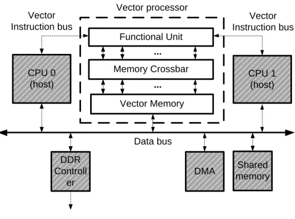
The general structure of the VP is described in Figure 6. The VP has three major parts: A Functional Unit, a Memory Crossbar and a Vector Memory. The

Functional Unit is the part that decodes and executes instructions from the hosts. The Vector Memory is an on-chip memory that is tightly connected to the

Functional Unit via the Memory Crossbar. The VM can be accessed directly by the Functional Unit, via the Crossbar, or by external processors via a data bus [13].

Memory Crossbar Vector Memory CPU 1 (host) Data bus Functional Unit CPU 0 (host) DMA DDR Controll er Vector Instruction bus Vector Instruction bus ... ... Shared memory Vector processor

Figure 6 - Overview of the whole system showing a setup with two CPUs connected to the highlighted VP.

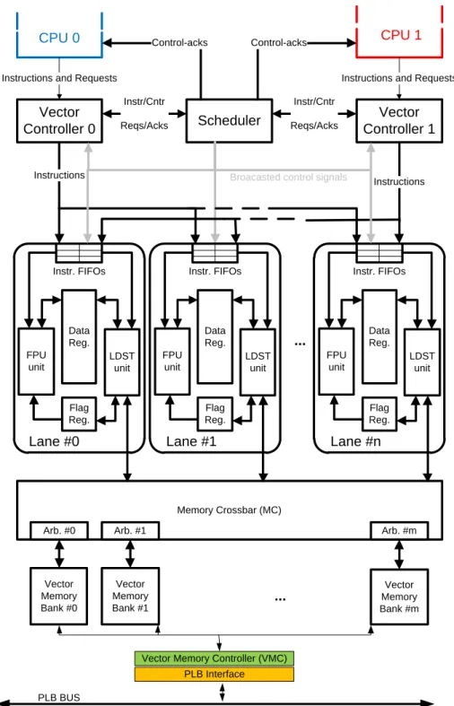
The vector processor is a typical coprocessor in the sense that it can receive instructions from a CPU and process them on its own. What is unique compared to others designs is that it can receive instructions from a number of CPUs/hosts in parallel. To make this possible there has to be some kind of arbiter that controls the flow of instructions from the different hosts. This is taken care of one Vector controller per host together with a Scheduler. These components are shown in Figure 7 where the VP is illustrated in detail [1].

(21)

The Scheduler controls the flow of instructions sent to the Vector lanes,

according to different scheduling schemes. The scheduler schedules according to one of the three different schemes, they are further described in section 3.2.2. To set up which scheme and vector length that should be used can each of the CPUs send a request (VPREQ). When the CPUs are finished executing a thread using the VP will it send a release request (VPREL). The Scheduler will answer these requests with a positive or negative acknowledgement to tell the CPU if the request was approved or not [1].

The Functional Unit from Figure 6 is composed from multiple Vector lanes. The Vector lanes are the ones that do the calculations and manipulate the data. The number of lanes is not fixed and the architecture is designed for an expandable amount of vector lanes. We have in the Test system chosen to have eight different lanes. A vector lane is described in detail in section 3.2.1 [1].

To connect the vector lanes with the vector memory there is a memory crossbar. The crossbar works like a switch, it connects a lane to that part of the vector memory the lane wants to access. For each bank in the vector memory there is an arbitrator to prevent collisions between memory accesses. The arbitrator uses a “round robin”-scheme to distribute the memory accesses between the lanes that want to access the same bank at the same time. The crossbar is an all-to-all network which can in a symmetric system connect all the lanes to one memory bank each for parallel transfer [1].

(22)

Vector Coprocessor Architecture Instr/Cntr Reqs/Acks Memory Crossbar (MC) Vector Memory Bank #0 Vector Controller 0 Vector Controller 1 Scheduler ... ... PLB Interface PLB BUS CPU 0 CPU 1

Vector Memory Controller (VMC) Instr/Cntr Reqs/Acks Arb. #0 Vector Memory Bank #1 Vector Memory Bank #m Arb. #1 Arb. #m ... Lane #n Data Reg. Flag Reg. FPU unit Instr. FIFOs LDST unit Lane #0 Data Reg. Flag Reg. FPU unit Instr. FIFOs LDST unit Lane #1 Data Reg. Flag Reg. FPU unit Instr. FIFOs LDST unit Instructions Instructions Control-acks Control-acks

Instructions and Requests Instructions and Requests

Broacasted control signals

(23)

 two Instruction First In, First Out (FIFO) queues, one for storing the instructions related with data processing and one for storing the instructions related with Load/Store operations.

 a Vector Register File (VRF) which consists in a subset of the VP VRF. Additionally, the operations executed on elements from VRF can conditioned by a bit called flag or mask. These bits form a Flag Vector Register File (FVRF)).

 a FPU (Floating-Point Unit) which executes different Single Precision Floating Point (SPFP) operations: add/subtract, multiply, absolute, negate, move. Also, the execution part implements flag operations (Read/Write) and may implement compare operations (parameterized design).

Additionally, the functionality of the FPU could be extended with other operations (fused multiply and add, division, square-root) by just plugging in other execution units that have standard interfaces according to VP Lane specifications [14].

A Load/Store unit that handles the transfers between VRF and VM. It supports unit-stride, non-unit stride and indexed memory accesses. Additionally, the LDST and the crossbar are designed to support inter-lane communication based on patterns located in Vector Registers. This instruction is called Vector Shuffle (VSHFL).The different instructions possible in this FPU and LDST are presented in Table 1. The Data register contains all the data that will be processed and that have been processed. The Flag register contains flags that are being used to mask operations done by the FPU.

Operation of the FPU Operation of the LD/ST

 Subtraction  Move

 Addition  Load

 Division  Store

 Multiplication  Load (Stride)

 Absolute  Store (Stride)

 Negate  Load (According to an index-vector)

 Store (According to an index-vector)

 Load (Single element)

 Store (Single element)

 Shuffle

(24)

Vector Coprocessor Architecture Lane M Data Reg. Flag Reg. FPU unit Instr FIFOs LDST unit

Figure 8 – A vector lane in VP. 3.2.2 Scheduling

As mentioned previously, there are different types of scheduling schemes for the scheduler. The scheduler is also responsible for proper configuration of each lane. Until now three different schemes have been designed. These are called Vector lane sharing (VLS), coarse-grain temporal sharing (CTS) and Fine-grain temporal sharing (FTS) [1].

The VLS means that the host processors will split the lanes equally between each other. So if there are two hosts they will get half of the lanes each. This will

basically work like they had one vector processor each but with half the lane width compared to the original size.

Timeslot Host A Host B

1 Using half the VP No access

(25)

1 Using the VP No access

2 No access Using the VP

4 No access No access

Table 3 – Example of usage of the VP according to CTS.

FTS is more advanced than the previous two. It will accept instructions from both processors and then mix the instructions. There is no extra overhead for the host and the communication between the host and the VP will be no different. The different hosts can work with different vector lengths and can have different priorities.

1 Using the VP No access

2 Using the VP (mixing instructions) Using the VP (mixing instructions)

4 No access No access

Table 4 – Example of usage of the VP according to FTS.

There are advantages and disadvantages of the schemes. The VLS will give better determination, because it is always possible for the hosts to access their part of the VP. The CTS will give higher performance for a single host because of exclusive usage of the whole VP. A disadvantage is that this will block the VP while it is being in use, and making it impossible for another host to access the VP. The advantage of the FTS is that the overall utilization of the VP can get very high. This is thanks to the possibility for the hosts to send instructions to the VP at the same time. The disadvantage is that it will not always give the same high speed as CTS from perspective of one host.

(26)

Vector Coprocessor Architecture 3.2.3 Instructions

This section is describing different instructions of the VP-instruction set. They are divided into FPU-instructions, LD/ST-instructions and Flag-instructions. The FPU-instructions are the instructions doing mathematical operations such as addition and subtraction while the LD/ST-instructions are controlling different kinds of memory operations. Some of the instructions can be used together with a so called flag register, which tells if the corresponding elements of the vector should be processed or not by the instructions. A flag can have the values “one” or “zero”. This means that an element with the value “one” in the flag register says that the element with the same index as the flag in the vector should be processed; a “zero” says the operation should not be executed and the results should not be committed. The Flag-instructions are instructions modifying these flag registers. The instructions are presented in three different tables below, each one corresponding to one of the instruction types.

In Table 5 are the FPU-instructions presented. We will scrutinize the VADD-instruction to give a greater understanding of the VADD-instructions. VADD is the mnemonic of an instruction adding two vectors. In the c-code it is implemented as a macro with some arguments as input. As for this example the macro would look something like this: VADD (VDest, VSrc1, VSrc2, VFlag). The VADD is an addition between two vectors. “VDest” tells in which vector register the result of the addition should be stored. “VSrc1” and “VSrc2” tells in which vector register the two vectors to be added are stored in. “VFlag” tells where the flag used together with the function is stored. A typical VADD could look like following: VADD(0,3,2,1). We can from this derive the following:

 The result will be stored in vector register #0.

 The addition will be done between elements of vector register #3 and elements from vector register #2.

(27)

Assembly mnemonic/syntax Description Flag _mask

VADD VDest, VSrc1, VSrc2, VFlag Adding two vectors.

VDest=VSrc1+VSrc2. Yes

VADD_S VDest, VSrc, VFlag, Type, Scalr Adding each element in a vector (VSrc) with a scalar (Scalr) and stores the result in VDest.

Yes

VSUB VDest, VSrc1, VSrc2, VFlag Subtracting two vectors. VDest=VSrc1-VSrc2.

Yes

VSUB_S VDest, VSrc, VFlag, Type, Scalr Subtracting each element in a vector

(VSrc) with a scalar (Scalr) Yes VMUL VDest, VSrc1, VSrc2, VFlag Multiplying corresponding elements in

VSrc1 and VSrc2 and stores it in VDest.

Yes

VMUL_S VDest, VSrc, VFlag, Type, Scalr Multiplying each element in a vector (VSrc) with a scalar (Scalr) and stores the result in VDest.

Yes

VNEG VDest, VSrc, VFlag Negate the elements in VSrc and store

it in VDest. Yes

VABS VDest, VSrc, VFlag Calculate the absolute value of each

element in VSrc and store it in VDest. Yes

Table 5 – FPU-instructions of the VP.

Table 6 present all the instructions of the LD/ST category. Like for the FPU an example is given for a LD/ST-instruction. In this case the VST-instruction is chosen. VST is storing a vector from a vector register to a memory address in the vector memory. An illustration by a macro would look as follows: VST(VSrc, VFlag, DestAddr). The “VSrc” tells in what vector register the vector that should be stored is located in. “VFlag” tells the flag register that is to be used.

“DestAddr” is the address in the memory where the vector should be stored. A VST could be used as in the following example: VST(1, 3, 0x0001AB00). The following can be obtained from this example:

 The vector that should be stored is located in vector register #1.

 The flag register #3 is used.

(28)

VMOV VDest, VSrc, VFlag Moves a vector from vector register

VSrc to vector register VDest. Yes VLD VDest, VFlag, SrcAddr Loads a vector from an address in the

memory space (SrcAddr) to a vector register (VDest).

Yes

VST VSrc, VFlag, DestAddr Stores a vector at an address in the memory space (DestAddr) from a vector register (VSrc).

Yes

VLDS VDest, VFlag, Stride, SrcAddr Loads a vector from an address in the memory space (SrcAddr) to a vector register (VDest) using strided access.

Yes

VSTS VSrc, VFlag, Stride, DestAddr Stores a vector at an address in the memory space (DestAddr) from a vector register (VSrc) using strided access.

Yes

VLDX VDest, VIndx, VFlag, SrcAddr Loads a vector from an address (SrcAddr) in memory space to a vector register. Compared to the VLD this one uses an additional register as an index. The corresponding element in VIndx is used as an offset relative to base address (SrcAddr). Base + offset gives the final address of the element in VM which is loaded in the the appropriate destination element.

Yes

VSTX VSrc, VIndx, VFlag, DestAddr Stores a vector to an address (DestAddr) in memory space to a vector register. Compared to the VST this one uses an additional register as an index. The corresponding element in VIndx is used as an offset relative to base address (DestAddr). Base + offset gives the final address to the position in the memory where to store the element with the same index in source vector (VSrc).

(29)

The Flag-instructions are presented in Table 7. Similar to the other instruction types there will be an example. VFLD is an instruction that loads a flag from a memory. The instruction looks like follows: VFLD(VFlagDest, SrcAddr). An example could be: VFLD(0, 0x0120_0000). From this we can derive:

 The flag vector will be stored in flag register #0.

 The flag vector will be loaded from memory position 0x0120_0000.

VFLD VFlagDest, Flag Loads flag provided as input to the instruction into a vector flag register (VFlagDest).

No

VFMOV VFlagDest, VFlagSrc Move a vector from one vector register (VFlagSrc) to another (VFlagDest). No VFNEG VFlagDest, VFlagSrc Negates the flag register VFlagSrc and

stores the result in VFlagDest. No

(30)

Method and Development tools

4 Method and Development tools

During this thesis work different kinds of development, simulations and analysis have been done. This chapter will explain different methods, tools and methods that have been used.

4.1 Hardware/Software Development

“Xilinx ISE Design Suite” has been used for all of the development. For the different part of the development different tools have been used. The “Xilinx ISE” is a suite of tools for synthesis and analysis of HDL-designs. The

“Embedded edition” which was used during the thesis work also includes

development tools for software. A list of the tools and a comparison of the Xilinx ISE Design suite can be found in Table 8 [17].

Features ISE

WebPACK Logic Edition Embedded Edition DSP Edition System Generator for DSP

Platform Studio and the Embedded Development Kit Software Development Kit MicroBlaze Soft Processor Design Preservation Project Navigator CORE Generator PlanAhead

ChipScope Pro and the ChipScope Pro Serial I/O Toolkit

Partial Reconfiguration* Power Optimization

ISE Simulator (ISim) (Limited) XST Synthesis

Timing Driven Place & Route, SmartGuide, and SmartXplorer

Table 8 – Comparison between the different versions of Xilinx ISE-tool suite. [17] The improvements of the architecture were designed in VHDL-code. The tool used was the “ISE Project Navigator 12.3”. It has an editor that was used for VHDL-coding. Furthermore the code was synthesised and analysed in the same tool.

The applications that were designed during the thesis work were written in ANSI-C. The development environment used for creating the applications was a tool

(31)

4.2 Prototyping Vector Processor Architecture

The whole system was prototyped on a FPGA. The device used was a FPGA from Xilinx, “Virtex-5 VLX110T” [19]. The host CPUs consist of soft-core processors from Xilinx of the type “MicroBlaze” [18], a 32-bits embedded RISC processor. The VP-architecture has been written in VHDL. There is also an external memory that is shared between the hosts and the VP. The memory is of the type BRAM. For this project we have chosen to use two CPUs/hosts, eight vector lanes on the vector processor and eight banks of Block RAM memory.

4.3 System Simulation and Analysis

The whole system (including software) was simulated using ModelSim SE 6.5e. By using the RTL system model derived from the VHDL design it was possible to obtain execution times of the applications. The execution times were calculated for each application by running part of the application and then estimating the runtime for a full execution. All simulations were run in ModelSim instead of on hardware, so that full logs and data could be observed.

For power estimation the XIilinx Xpower [20] tool was used. The input for the tool is the generated netlist. This software uses the “.vcd”-files generated after synthesis, translate, map and “place and route”.

Using the ModelSim software also made it possible to analyse the applications. This was made possible by running the RTL simulation and using the results together with the Waveform viewer included in ModelSim. The Waveform viewer (example shown in Figure 9) gives the developer a tool for seeing all the

transmissions and communication in the simulated system. It is then possible to see what instructions and data that were transferred during the simulation. By calculating the expected outcome from calculations with Matlab it was possible to verify the correct functionality of the design and applications.

(32)

Figure 9 - Example of a waveform illustration showing execution of a VHDL application.

For the extension of the architecture (described in Chapter 1) done during the thesis work there also had to be simulations. These were also done in ModelSim. Together with a test bench written in VHDL the extension could be simulated and analysed.

(33)

Application Development and Performance Evaluation

5 Application Development and

Performance Evaluation

This chapter explains the development process of the applications that were designed during the thesis work and also the applications implementation in detail. Pseudo code for the applications is presented but also explanations in detail with illustrating examples for easier understanding. It also presents the results of the simulations and some of the theory behind the performance and performance enhancement achieved by using the vector processor as an accelerator.

As preparation for the project literature study covering vector mathematics in general and vector processors in particular were to be carried out.

5.1 Application development process

During the project several applications have been implemented to run on the Test architecture for the purpose to verify functionality and to benchmark the

performance of the Vector unit. For each application different scenarios have been generated. The different scenarios have been varied with these factors:

 Various vector lengths: 32, 64 or 128.

 Multiple threads in the Vector processor: Multiple processors sending instructions will result in separate threads in the Vector processor. In this case two processors using different memory space and therefore

independent threads with no data dependency.

 Loop unrolling: The unrolling of loops in the applications helps improve the performance of the application by decreasing loop overhead.

 Scheduling schemes: Simply usage of different scheduling schemes (CTS, VLS, and FTS) in the Vector processor to compare their efficiency.

The process of developing an application is described in Figure 10. Every application was written so that they should be as general as possible so that they easily could be ported to different kinds of processors. This was made possible by the transparency of the vector instructions to the programmer. This means that vector registers were transparent so that two processors could use e.g. vector register 1 but would still operate on different physical vector registers. This is handled by the register renaming feature of the Vector processor. Thanks to this the mapping of the applications to each of the CPUs basically resulted in defining the memory space for data storage.

(34)

New Application

Partitioning of Application

(Manual)

Code CPU 1 … Code CPU N

Analyse code to identify vector operations (Manual) ... Modify and rewrite code using vector operation Compile c-code Generate Hex-code of c-Hex-code and data to be stored on local and shared memory Execution of code on Parallel processors sharing

vector co-processor Shared vector memory ... ... ...

Figure 10 – Flowchart describing an Application Development and Execution process.

(35)

Application Development and Performance Evaluation ∑ (2)

Our application was implemented for multiplication of two n×n matrices. While there is no instruction for adding up all the elements in a vector implemented in the Vector processor the algorithm had to be designed with that in mind.

Something that also had to be considered was the amount of space that was available in the vector memory (64KB for 8x8 lanes configuration).

5.2.1 Mapping of application on architecture

The different CPUs do computations on different sub-sets of the same matrix multiplication. This means that they will compute different parts of the resulting matrix but some matrix elements will be shared, due to dependencies in the algorithm. The instructions will still be mixed in the VP according to the scheduling scheme that is used.

The CPU(s) sends a request of a chosen vector length that the VP will work with. After that request the CPU sets up a memory transfer that is done by a shared DMA-unit. When there are two CPUs only one of them will set up the initial transfer. The initial DMA-transfer transfers the parts of the Matrices that are needed to start the Matrix multiplication. After that they will wait until the transfer is done. When done the processor(s) will start the matrix multiplication.

The implementation was chosen so that if a vector is bigger than thirty*vector length it is split into sections, as in Figure 11. This limit is due to size of vector memory. The sections of the resulting matrix are calculated sequentially. Every section is of the size of thirty rows of the length equal to the vector length that was requested by the CPU. The thirty rows are in computation at the same time. This will enable to achieve per thread high level of data parallelism by using loop-unrolling and increased Vector Lengths.

(36)

Application Development and Performance Evaluation Vector length 3 0 r o w s 2 n 1 … Matrix size M a tr ix s iz e

Figure 11 – Illustrating how a large matrix-multiplication problem is split into sections.

While there is no instruction in the vector processor to add up elements of a row, there had to be, in some sense, a special approach to get around this. This was done by accumulating the thirty results from each row by adding the result of a scalar-vector multiplication with each of the scalar on row with every row (of vector length) in the current column from the top of the section to the bottom of the matrix. In this way a scalar-matrix multiplication can be done in the vector processor compared to a scalar-scalar-multiplication which would have been done in with a scalar-processor. This means that 30 scalar-vector multiplications are done to the same vector per iterations. Each of these results is accumulated to the corresponding “accumulator”. In the next iteration the next vector is multiplied with the thirty scalars in the next column until all row vectors have been

processed. The choice of thirty rows was because of the maximum of 32 registers when using the vector length 256. The two extra registers not used as

accumulators were used for temporal storage during the matrix multiplication. [

_]

[ ]

(37)

The result is to 30 scalar-vector multiplications per iteration and 30 vector-adds to accumulate the result

[ ] [ ] [ ] In the second iterations there will be another 30 scalar-vector multiplications

[ ] [ ] [ ] This will be repeated until all rows in the column have been used. This is illustrated in Figure 12. Vector length 3 0 r o w s 1 Matrix size M a tr ix s iz e

(38)

To give more understanding, I present an example and comparison between sequential and parallel calculation. The values of the matrix multiplication that will be done, including values, is presented in (3). In the parallel example there is three accumulators compared to in the real application were thirty accumulators were used. [ ] [ ] [ ] (3) In

Figure 14 a timing diagram that explains the execution of the previous examples is shown. The x-axis shows the time and the y-axis what process/function is being executed. According to the chosen vector length of three in the example it can be seen that there are three numbers executed in parallel in the same time unit for the parallel example. This correlates with the total time for the execution as the

(39)

Sequential 3-by-3 matrix multiplication Parallel 3-by-3 matrix multiplication

No. Calculation Current values No. Calculations Current values

1 2 3 4 5 6 7 8 9 10 11 12 13 14 15 16 17 18 19 20 21 22 23 24 25 26 27 28 29 30 31 32 33 34 35 36 37 38 39 40 41 42 43 44 45 5*1 = 5 2*7 = 14 3*8 = 24 5+14 = 19 19+24 = 43 5*3 = 15 2*9 = 18 3*6 = 18 15+18 = 33 33+18 = 51 5*4 = 20 2*5 = 10 3*2 = 6 20 + 10 = 30 30 + 6 = 36 4*1 = 4 9*7 = 63 1*8 = 8 4+63 = 67 67+8 = 75 4*3 = 12 9*9 = 81 1*6 = 6 12+81 = 93 93+6 = 99 4*4 = 16 9*5 = 45 1*2 = 2 16+45 = 61 61+2 = 63 7*1 = 7 6*7 = 42 8*8 = 64 7+42 = 49 49+64 = 113 7*3 = 21 6*9 = 54 8*6 = 48 21+54 = 75 75 + 48 = 123 7*4 = 28 6*5 = 30 8*2 = 16 28+30 = 58 58+16 = 74 [ ] [ ] [ ] [ ] [ ] [ ] [ ] [ ] [ ] 1 2 3 4 5 6 7 8 9 10 11 12 13 14 15 16 17 18 5*[ ] = [ ] [ ] + [ ] = [ ] 4*[ ] = [ ] [ ] + [ ]= [ ] 7*[ ] = [ ] [ ] +[ ] = [ ] 2*[ ] = [ ] [ ] + [ ] = [ ] 9*[ ] = [ ] [ ] [ ] [ ] 6*[ ] = [ ] [ ] [ ] [ ] 3*[ ] = [ ] [ ] [ ] [ ] 1*[ ] = [ ] [ ] [ ] [ ] 8*[ ] = [ ] [ ] [ ] [ ] [ ] [ ] [ ] [ ] [ ] [ ] [ ] [ ] [ ]

Figure 13 - Showing a comparison between a sequential matrix multiplication and a parallel matrix multiplication. It takes 45 scalar instructions to do this matrix multiplication, but only 18 vector instructions. The advantage of a VP is obvious and would be even more obvious with a larger vector size, e.g. eight, which is the

(40)

Application Development and Performance Evaluation 1-3 4-6 7-9 1-3 1-3 4-6 4-6 7-9 Mult Add 1 2 3 4 5 6 7 8 ... 7-9 7-9 14 15 1 1 1 1 1 2 2 2 Mult Add 1 2 3 4 5 6 7 8 ... 9 9 44 45 Sequential Parallel Time units Process Process Time units

Figure 14 – Timeline describing the execution of the sequential and the parallel execution of the previously presented example, assuming one core using the VP with CTS. The numbers within the blocks says which element(s) is/are executed. 5.2.2 Pseudo code of mapped application

MAIN()

1 Request access/vector length of vector processor. 2 MATRIX_MULT(memAddr, vectorLength)

MATRIX_MULT(memAdd, VectorLength) 1 for each section

2 for each column in section 3 Fetch data via DMA

4 Load vector to vector register

5 for each scalar in column and section 6 scalar * ptrToCurrVector

7 Add result to according accumulator

(41)

Application Development and Performance Evaluation 5.2.3 Performance evaluation of the application

Looking at the equation (2) we can derive that the time complexity of the

sequential matrix multiplication algorithm is O( ). Looking at Figure 15 we can instead derive that the time complexity for the parallel design will be O( ) when N>8 or O( ) when N≤8 (Assuming that the vector length is 8).

When looking at Figure 13 we can see that the calculations correlate with the theory. In the example the vector length is 3. The theory then says that if N≤3 we will get O( ) for the parallel and O( ) for the sequential part.

Totally 27 different scenarios were created. Performance of some of the scenarios is presented in Table 9. In the table the utilizations of the FPU-unit and the Load/Store unit is shown. Further the execution time of processing one element in the Matrix multiplication. In the last column the speedup relative the

application running on one CPU presented, in this case a soft core scalar

processor from Xilinx called MicroBlaze. We can see that using the VP can give a huge performance boost. In the best case 62 times speedup compared to the reference design was achieved.

Scheduling Scenario Average utilization (%) Execution _{Time (µs)} Speedup

FPU LDST

N/A One MicroBlaze w/o VP N/A N/A 130.90 1 N/A Two MicroBlaze w/o VP N/A N/A 65.45 2 CTS VL=32, no loop unrolled 20.37 VL=32, unrolled once 33.94 20.70 34.50 10.09 6.03 12.97 21.71

VL=128, unrolled once 68.30 69.51 3.01 43.49 FTS VL=32, no loop unrolled 40.59 VL=32, unrolled once 67.09 41.29 68.20 5.055 3.048 25.89 42.95 VL=128, unrolled once 97.32 98.91 2.102 62.27 VLS VL=32, no loop unrolled 33.83 VL=32, unrolled once 53.51 34.34 54.45 6.086 3.791 21.51 34.53 VL=128, unrolled once 81.88 83.40 2.494 52.48

N/A GPP Xeon N/A N/A 20.56 6.36

Table 9 – Performance comparison of Matrix multiplication application. Table 10 shows the power and energy consumption of the system when running Matrix multiplication. This is a comparison of some scenarios with differences of vector length and code optimization in the context of loop unrolling. All of these scenarios are running the system of two CPU together with the VP. The different scenarios are also running different scheduling schemes. We can here see that there is a substantial difference between the different scenarios. The most efficient is the one with the FTS-scheme and VL of 128. What can be seen in the table is also that the differences in dynamic power are not very big in between the scenarios compared to the differences in total power. This means that the differences in total energy budget are caused by static energy. The static power correlates with the execution time, this tells us that the scenarios that’s using a low total power also is fast and in that way saves static energy.

(42)

Scheduling Scenario Dynamic _{Power (mW)} Energy (nJ) _{Dynamic Total} nJ/FLOP CTS VL=32, no loop unrolled 166.22 VL=32, unrolled once 296.69 1677.16 1787.85 5713.16 4198.25 2.789 2.049

VL=128, unrolled once 555.02 1671.16 2875.68 1.404 FTS VL=32, no loop unrolled 332.86 VL=32, unrolled once 610.20 1682.61 1859.89 3704.60 3079.08 1.808 1.503 VL=128, unrolled once 793.65 1668.25 2509.05 1.225 VLS VL=32, no loop unrolled 311.86 VL=32, unrolled once 513.59 1897.98 1947.02 4332.38 3463.42 2.115 1.691 VL=128, unrolled once 668.76 1667.89 2665.49 1.301

Table 10 – Power consumption comparison Matrix multiplication application.

5.3 LU-Decomposition

LU-decomposition (also called LU factorization) is a process to factorize a N*N-matrix into two matrices, one lower triangular N*N-matrix and one upper triangular matrix, as illustrated in (4). In the lower triangular matrix, all the elements above the diagonal are 0´s. Similarly all the elements below the diagonal in the upper triangle are 0´s [ ] [ ] [ ] (4)

5.3.1 Mapping of application on architecture First version

The factorization was carried using Gauss Elimination method. The lower matrix will be the result of a forward substitution. The divisions were all done in the CPU in the first version. Result of a forward substation will be used to create the upper matrix with back substitution. These operations are done with the help of the vector processor. The LU-decomposition application is designed using a recursive algorithm. It will adjust the vector size processed by the VP according to the decreasing size of the upper matrix and is illustrated in Figure 16. This means that the vector size requested will decrease according to the decreasing row length of the upper matrix. For example when using vector length 64 and the row length have decreased to 32 vector length 32 is requested.

(43)

Figure 16 - Graphical illustration of the recursive algorithm of LU decomposition Second version

In a second version division made by the microcontroller have been replaced by VP-division. This division is done on the whole active part of the column. This should be compared with when division was made by the microcontroller inside the iteration where every division was done sequentially. During the process of designing the applications there were modifications of the vector processor. These modifications added support vector lengths of any integer between 1 and

requested vector length. In the second version was the functionality “Any-VL” of the VP also used. This means that Any VL length shorter than the originally VL length could be requested for the arithmetic operations. This saves one cycle for every row eight shorter than the previous request. Eight in our case because the number of vector lanes is eight. So instead of making a request of vector length 32 after previously having 64 we can instead make an “Any-VL” request every eight step: 56, 48, 40 and so on. This made it possible to make the LU-decomposition even more efficient.

(44)

To show the difference between calculating the LU decomposition sequential and parallel two small examples are presented. The matrix used in the example is presented in Equation (5). The examples are presented in Table 11 and Table 12. The examples are using the same 3-by-3 matrix, but the parallel example will do the computation in six cycles compared to the sequential example with eleven cycles. This scenarios assumes that the VL used is 3 and that the VP used have at least 3 lanes. Obviously the gain will be even greater when using bigger matrices and VL, assuming the VP has a greater number of lanes.

[ ] [ ] [ ] (5)

Sequential 3-by-3 LU Decomposition

No. Calculation Result(L/U)

1 2 3 4 6/4=1,5 6 – 1,5*4=0 3 – 1,5*3=-1,5 8 – 1,5*5=0,5 [ ] [ ] 5 6 7 8 8/4=2 8-2*4=0 7-2*3=1 2-2*5=-8 [ ] [ ] 9 10 11 1/-1,5 = 0,666 1-0,666*-1,5=0 -8*-0,666*0,5=-7,666 [ ] [ ] Table 11 – Example showing a sequential computation of LU decomposition. Parallel 3-by-3 LU Decomposition

No. Calculation Result(L/U)

1

2 6/4=1,5 [ ] 1,5*[ ] [

(45)

Application Development and Performance Evaluation 5.3.2 Pseudo code of mapped application

MAIN()

1 transfer matrix from BRAM to VM at memAddr 2 LU_DECOMP(memAddr, vectorLength);

LU_DECOMP(memAdd, VectorLength) 1 for each colon in the matrix

2 if number of colons computed = vectorLength/2 3 calculate the newMenAddr

4 LU_DECOMP(newMemAddr, vectorLength/2) 5 else

6 for rownumber = current colon to last row

7 div_res ← (current element)/(first element in colon) 8 mul_res ← res*top_row

9 current row – mul_res

10 store div_res for current element as part of L-matrix 11 store mul_res as part of the current row in the U-matrix

Figure 17 – Pseudo-code describing the implementation of the first version. Bold text indicates operations executed by the vector processor.

MAIN()

1 transfer matrix from BRAM to VM at memAddr 2 LU_DECOMP(memAddr, vectorLength);

LU_DECOMP(memAdd, vectorLength) 1 for each colon in the matrix

2 if number of colons vectorLength-8 3 calculate the newMemAddr

4 LU_DECOMP(newMemAddr, vectorLength-8); 5 else

6 load the vector of elements/scalars that should be divided 7 divide the vector/ arrays of scalars with top scalar

8 strided LD/ST back results 9 wait until store is done

10 for rownumber = current colon to last row 11 load the current row

12 multiply row with corresponding scalar

13 substract the row with result from prev multiply 14 store back result

15 end for 16 end if 17 end for

Figure 18 - Pseudo-code describing the implementation of the second version. Bold text indicates operations executed by the vector processor.

(46)

Application Development and Performance Evaluation 5.3.3 Performance evaluation of the application

The theoretical time complexity for LU decomposition is . Using parallel computing it has been reported that the time complexity can be reduced to [22].

Twelve different scenarios were generated from the LU decomposition. The performance of them is presented in Table 13. Likewise the performance table of the Matrix multiplications the utilization of FPU-unit and the Load/Store-unit is presented. Further the execution time per row and the estimated execution time of the entire matrix (128x128) are presented. In the last column shows the speedup relative the reference design (soft core scalar processor MicroBlaze). The

execution time of the operations on a Xeon-processor has been added to give extra understanding of the size of the speed-up.

In the results in Table 13 we can see that the FTS gives the fastest execution. It is more than four hundred times faster than the execution of the math operation in one MicroBlaze. The reason why the speedup is quite big is due to several reasons. One reason is that the scalar core is not able to use the cash memory efficiently and therefore the cash misses cause access latency resulting high execution time. In opposition to that the VP implementation uses DMA transfers instead of caching to transfer data in and out.

Scheduling Scenario Average utilization (%) Execution Time (µs) per row of size VL Execution Time (µs) for entire LU Dec. Speedup FPU LDST

N/A One MB _{w/o VP} N/A N/A N/A 1,034,340 1 N/A Two MB _{w/o VP} N/A N/A N/A 517,170 2

CTS VL=16 4.73 5.34 0.632 5,137 201.35 VL=32 9.88 10.36 0.632 VL=64 20.11 20.42 0.632 VL=128 40.44 40.54 0.632 FTS VL=16 8.32 8.54 0.312 2,568 402.78 VL=32 18.74 21.08 0.316 VL=64 39.93 41.36 0.316 VL=128 81.05 82.30 0.316 VLS VL=16 8.70 11.11 0.320 3,522 293.68 VL=32 19.05 21.03 0.316 VL=64 39.62 41.05 0.316 VL=128 53.86 54.95 0.472