Improvements of U-pipe Borehole
Heat Exchangers
José Acuña
Licentiate Thesis 2010
KTH School of Industrial Engineering and Management Division of Applied Thermodynamic and Refrigeration
ISBN 978-91-7415-660-7 Trita Refr Report No 10/01
ISSN-1102-0245
ISRN KTH/REFR/10/01-SE © José Acuña
Abstract
The sales of Ground Source Heat Pumps in Sweden and many other countries are having a rapid growth in the last decade. Today, there are approximately 360 000 systems installed in Sweden, with a growing rate of about 30 000 installations per year. The most common way to ex-change heat with the bedrock in ground source heat pump applications is circulating a secondary fluid through a Borehole Heat Exchanger (BHE), a closed loop in a vertical borehole. The fluid transports the heat from the ground to a certain heating and or cooling application. A fluid with one degree higher or lower temperature coming out from the borehole may represent a 2-3% change in the COP of a heat pump system. It is therefore of great relevance to design cost effective and easy to install borehole heat exchangers. U-pipe BHEs consisting of two equal cylin-drical pipes connected together at the borehole bottom have dominated the market for several years in spite of their relatively poor thermal per-formance and, still, there exist many uncertainties about how to optimize them. Although more efficient BHEs have been discussed for many years, the introduction of new designs has been practically lacking. How-ever, the interest for innovation within this field is increasing nowadays and more effective methods for injecting or extracting heat into/from the ground (better BHEs) with smaller temperature differences between the heat secondary fluid and the surrounding bedrock must be suggested for introduction into the market.
This report presents the analysis of several groundwater filled borehole heat exchangers, including standard and alternative U-pipe configura-tions (e.g. with spacers, grooves), as well as two coaxial designs. The study embraces measurements of borehole deviation, ground water flow, undisturbed ground temperature profile, secondary fluid and groundwa-ter temperature variations in time, theoretical analyses with a FEM soft-ware, Distributed Thermal Response Test (DTRT), and pressure drop. Significant attention is devoted to distributed temperature measurements using optic fiber cables along the BHEs during heat extraction and heat injection from and to the ground.
Keywords: Borehole Heat Exchangers, Distributed Thermal Response Test, Ground Source Heat Pumps.
Preface
It is for many people unknown what a Swedish licentiate of engineering degree is. What I know is that one of the ideas with this degree is to of-fer a shorter option for specialized education and thereby attract more students into research and doctoral education programs. Although it can be voluntary, the licentiate level is sometimes used to demark that about half of the doctoral studies have been completed, depending on every particular project. The financial support is often a determinant factor that influences whether choosing a student for a licentiate instead of a doctoral program. Independently of this, what I have witnessed myself is that an un-measureable very positive amount of knowledge of different kinds is obtained during this education period.
This licentiate of engineering thesis is based on most of the work from the first two and a half years of research carried out at the energy tech-nology department at KTH. The project title is “Efficient Use of Energy Wells for Heat Pumps” and it is part of the Swedish applied refrigeration and heat pump research program EFFSYS2. It is ongoing since the mid-dle of 2007 on a 80% time basis. The project target is to point out rec-ommendations for design of Borehole Heat Exchangers in order to im-prove the Coefficient of Performance of Ground Source Heat Pumps by 10-20%. It is estimated that applying the project results could imply an electric energy saving of about 0.2-0.4 TWh/yr in Sweden. The work done so far indicates that the project is developing on the right track and I personally think that reaching the target seems relatively easy to achieve.
The project has been characterized by a very big interest from the indus-try and from the community. A total of 33 partners have followed its progress, some from the beginning and some have joined later. We have all learned a lot. I even think that we have contributed to stimulating the market towards the beginning of a new era with more efficient Borehole Heat Exchangers!
This report is part of my Ph.D. studies and it gives the continuation of the project a strong background to be oriented upon, given that a consi-derable part of the work has been completed and reported. The defense of this report also gives me valuable training for the Ph.D. disputation!
A c k n o w l e d g e m e n t s
This project has been characterized by a high degree of openness and collaboration. The Swedish Energy Agency is greatly acknowledged for financing the project together with all our industrial partners:
Aska rör, Avanti system AB, Brunata, COMSOL AB, COOLY, Cupori AB, DTI, ETM Kylteknik, EXTENA, Geosigma, GRUNDFOS, Höga-lids elektriska, Hydroresearch AB, IVT, LOWTE, Lämpöässä, Manil Bygg, Mateve Oy, MuoviTech, NeoEnergy, NIBE, Nordahl fastigheter, PEMTEC, SEEC AB, SVEP, SWECO, THERMIA, Thoren, UPO-NOR, WILO. Special thanks to Palne Mogensen, Tommy Nilsson, Jan-Erik Nowacki, Kenneth Weber, and Brage Broberg!
Several house owners and residents have kindly allowed us to carry out the research at their buildings. Thank you! I would also like to extend a warm gratitude to people who have helped during many fun days of planning and borehole heat exchanger installation: Peter Hill, Mikael Nordahl, Benny Andersson, Benny Sjöberg, Klas Andersson, Hans Alex-anderson, Michael Klasson, Jan Cederström, Åke Melinder, Björn Kyrk, Sam Johansson, Mauri Lieskoski, Johan Wasberg, Jussi, Slawek, Claudi, Samer, Rashid, Stina, Hatef, Julia, Jesus, Tomas, Leoni, Maria, Andreas, Lukas, Tommy and Charles.
Thanks to all my colleagues from KTH for making the lab a nice envi-ronment where smiles never lack. A special appreciation to my supervi-sor Prof. Björn Palm, for his time, support, good will, and orientation! I would like to dedicate this report to my parents Yajaira and José, my sister Fatima, to grandma Mercedes, and my wife Dominika, for their pa-tience, infinite support and comprehension.
Thank you all for your positive spirit. You are all sources of inspiration! I hope we all keep healthy so that we can continue witnessing the devel-opment of this study.
P u b l i c a t i o n s
Most of the material presented in this report is from the articles pub-lished in conference proceedings, as listed below. However, some results and analyses are hereby published for first time.
1. J. Acuña, B. Palm. Comprehensive Summary of Borehole Heat Ex-changer Research at KTH. Accepted for presentation at the Confer-ence on Sustainable Refrigeration and Heat Pump Technology, Stockholm, 2010.
2. J. Acuña, P. Mogensen, B. Palm. Evaluation of a Coaxial Borehole Heat Exchanger Prototype. Accepted for presentation at the 14th ASME IHTC International Heat Transfer Conference, Washington D.C 2010.
3. H. Madani, J. Acuña, J. Claesson, P. Lundqvist, B. Palm. The Ground Source Heat Pump: A System Analysis with a Particular Focus on the U-pipe Borehole Heat Exchanger. Draft. Accepted for presentation at the 14th ASME IHTC International Heat Transfer Conference, Washington D.C 2010.
4. J. Acuña, B. Palm. A Novel Coaxial Borehole Heat Exchanger: De-scription and First Distributed Thermal Response Test Measure-ments. World Geothermal Congress, Bali 2010.
5. J. Acuña, B. Palm. Local Heat Transfer in U-pipe Borehole Heat Ex-changers. COMSOL Multiphysics Conference, Milano 2009.
6. J. Acuña, P. Mogensen, B. Palm. Distributed Thermal Response Test on a U-pipe Borehole Heat Exchanger. The 11th International Confer-ence on Energy Storage EFFSTOCK, Stockholm 2009.
7. J. Acuña, B. Palm. Experimental Comparison of Four Borehole Heat Exchangers. 8th IIR Gustav Lorentzen Conference, Copenhagen 2008.
8. J. Acuña, B. Palm, P. Hill. Characterization of Boreholes: Results from a U-pipe Borehole Heat Exchanger Installation. 9th IEA Heat Pump Conference, Zurich 2008. s4-p19.
In addition, some of the results have popularly been disseminated at the following magazines from different countries:
1. J. Acuña. Efficient Use of Energy Wells for Heat Pumps. GeoCon-neXion Magazine. Canada, Fall 2009.
2. J. Acuña. Slang intill bergväggen ger effektivare värmeväxling. Hus-byggaren, nr 6 2009.
3. T. Tenfält. Forskningsprojekt Ska Ge Effektivare Bergvärme, VVS Fo-rum no. 1, 2009
4. Ελλáδa (Artikel om svenska energilösningar publicerad i Grekland).
5. T. Tenfältl. Bättre bergvärmeanläggningar med optimal energybrunnar. Borrsvängen nr 1/2009.
6. J. Acuña. Bergvärmepumpar Kan Göras Ännu Mer Effektiva, Ene-gi&Miljö no 3, 2008.
7. Dagens Nyheter. Bergvärme inte lika populärt längre. Citation from interview to J. Acuña, April 13th, 2008.
8. U. Hammarsträng. Ny energikollektor med världspatent. Slussen Biz, September 23rd, 2008.
9. Hur bra kan ett borrhål bli? Interview till J. Acuña. SVEP NYTT nr 3, 2008.
Several oral presentations and posters about this project and its results have also been presented at the following events:
• Geothermal PhD student day, Potsdam 2010. • EFFSYS2 days 2007, 2008, 2009.
• Sveriges energiting - Framtidens värmepumpar. Stockholm, 2009. • Nordic Climate Solutions conference. Copenhagen, 2008
• Nordbygg. Stockholm, 2008.
• Nya energilösningar för områdesbyggande seminar, Vasa, 2008. • Ground Source Heat Pumps Workshop. Bilbao, 2008.
More information about the project can be found online at
http://www.energy.kth.se/energibrunnar and http://www.effsys2.se
A b b r e v i a t i o n s a n d N o m e n c l a t u r e
BHE… Borehole Heat Exchanger
COP… Coefficient of Performance [-]
COPheating… Coefficient of Performance in heating mode [-]
DTS… Distributed Temperature Sensing
DTRT… Distributed Thermal Response Test
GSHP… Ground Source Heat Pump
TRT… Thermal Response Test
Cp… Specific heat capacity [J/kgK]
∆Tf-bhw… Logarithmic mean temperature difference [K]
E
E … Pumping power [W]
… Compressor power [W]
∆P… Pressure drop [Pa]
∆Pf… Pressure drop due to friction [Pa]
∆T… Temperature difference [K]
f… Friction factor [-]
h … Convection heat transfer coefficient [W/m2K]
L … Borehole or pipe length [m]
Nu… Nusselt number [non-dimensional]
ηpump… Pump efficiency [-]
q… Thermal power [W]
q’… Thermal power per unit length [W/m]
q’’… Thermal power per unit area [W/m2]
qge
Q … Power supplied at the condenser side of the heat pump [W]
o’’… Geothermal heat flux [W/m2]
Pr… Prandtl number [non-dimensional]
Re… Reynolds number [non-dimensional]
re … external radius for contact resistance calculation [m]
rext … outer pipe radius [m]
rbh … borehole radius [m]
rp … pipe radius [m]
rrock … rock radius at a given distance from the borehole center [m]
R... Radial distance [m]
Rb… Borehole thermal resistance [K m/W]
Res... Thermal resistance [K m/W]
Rf-rock... Fluid to rock thermal resistance [K m/W]
Rrock... Rock thermal resistance [K m/W]
t… time [sec]
Tbhw… Borehole wall temperature [˚C]
Tin… Inlet temperature at the down or up going BHE flow channel [˚C]
To… Temperature where the geothermal gradient starts [˚C]
Tout… Outlet temperature at the down or up going BHE flow channel [˚C]
Tf … Fluid mean temperature [˚C]
Trock … Rock temperature [˚C]
Tm … Mean reference fluid temperature at cross section [˚C]
Ts
V… Volumetric flow rate [m3/s]
… Pipe internal surface temperature [˚C]
w… Velocity [m/s]
z… depth [m]
α … thermal diffusivity [m2/s]
β … integration variable [-]
δgap… gap distance for constant resistance calculation [m]
γ… Eulers constant [0.5772…]
γf… Variable for fiber optic measurement calculation [K]
η… Efficiency [-]
ν… Kinematic viscosity [m2/s]
λ… Thermal conductivity [W/m K]
Table of Contents
ABSTRACT 3
PREFACE 4
ACKNOWLEDGEMENTS 5
PUBLICATIONS 6
ABBREVIATIONS AND NOMENCLATURE 7
TABLE OF CONTENTS 10
INDEX OF FIGURES 11
INDEX OF TABLES 14
1 INTRODUCTION – BASIC CONCEPTS 15
1.1 GROUND SOURCE HEAT PUMPS 15
1.2 THERMAL PROCESSES IN THE GROUND 18
1.3 SECONDARY WORKING FLUID FLOW 20
1.3.1 Hydrodynamic considerations 21
1.3.2 Thermal considerations 21
1.4 THERMAL RESISTANCES IN BHES 23
1.5 THERMAL RESPONSE TEST 26
1.6 BOREHOLE HEAT EXCHANGERS-STATE OF THE ART 29
1.6.1 U-pipe BHEs 30
1.6.2 Coaxial BHEs 32
1.7 DISTRIBUTED TEMPERATURE MEASUREMENTS 33
2 EXPERIENCES WITH U-PIPE BHES 39
2.1 DESCRIPTION OF THE INSTALLATION 39
2.2 TEMPERATURES DURING HEAT PUMP OPERATION 43 2.3 DISTRIBUTED THERMAL RESPONSE TEST 50
2.4 DISTRIBUTED PRESSURE MEASUREMENTS 57
3 EXPERIENCES WITH ALTERNATIVE U-PIPE BHES 61
3.1 THEORETICAL EVALUATION 62
3.2 EXPERIMENTAL EVALUATION 67
4 EXPERIENCES WITH COAXIAL BHES 76
4.1 AN ANNULAR COAXIAL BHE- FIRST PROTOTYPE 76 4.2 COAXIAL PROTOTYPE WITH FIVE EXTERNAL FLOW CHANNELS 80
5 CONCLUSIONS 90
I n d e x o f F i g u r e s
Figure 1. Three undisturbed ground temperature profiles in Stockholm, Sweden 15 Figure 2. U-pipe BHE 16 Figure 3. GSHP basic sketch 17 Figure 4. Illustration of thermal resistance components in a BHE 24 Figure 5. Pipe thermal resistance as a function of its thermal conductivity 24 Figure 6. The first Thermal Response Tester. Mogensen (1983) 27 Figure 7. Illustration of a heat injection thermal response test 28 Figure 8. TRT equipment connected to a borehole for DTRT 29 Figure 9. The data logging equipment 34 Figure 10. Thermocouple connection sketch 34 Figure 11. Ice bath for fiber optic calibration 36 Figure 12. Sketch of the fiber optic loop in two BHEs 36 Figure 13. Example of DTS measurement during calibration 37 Figure 14. Overview of the borehole components 40 Figure 15. Deviation of the borehole towards north and east direction 41 Figure 16. Deviation of the borehole with regard to the vertical direction 41 Figure 17. Ground water flow along the borehole length 42 Figure 18. Undisturbed Temperature profile 42 Figure 19. Fluid temperatures at different depths during heat pump operation 44 Figure 20. Temperature profile during heat pump operation 45 Figure 21. Secondary fluid temperature profile during borehole operation cycle 46 Figure 22. Fluid and ground water temperatures during the system start up 47
Figure 23. Temperatures and specific heat extraction at 0.3 l/s 48 Figure 24. Temperatures and specific heat extraction at 0.4 l/s 48 Figure 25. Temperatures and specific heat extraction at 0.5 l/s 48 Figure 26. Borehole Sectioning 50 Figure 27. Measurement room while carrying out the DTRT 51 Figure 28. Temperatures measured with the thermocouples during the DTRT 52 Figure 29. Average temperatures during the first three phases of the DTRT 53 Figure 30. Power supplied in each BHE section during the heating phase 54 Figure 31. Average temperatures in each section during the heat injection phase 55 Figure 32. Average temperatures in each section during the borehole recovery phase 55 Figure 33. (a)Thermal resistance and (b)Thermal conductivity in each section 56 Figure 34. Distributed pressure measurement experimental rig 58 Figure 35. Illustration and picture of the pressure tabs 58 Figure 36. Connection of the pressure meter to the pipe 59 Figure 37. Pressure values before subtracting the height difference between points 59 Figure 38. Pressure values accounting for the height difference between points 60 Figure 39. Picture of 38 mm spacers 61 Figure 40. Picture of BHE instrumented with 13 mm spacers 61 Figure 41. Three pipe BHE 61 Figure 42. U-pipe with grooves 61 Figure 43. Pipes apart 65 Figure 44. Pipes aside together 65 Figure 45. Pipes together aside 2 65
Figure 46. Pipes together centered 65 Figure 47. 13 mm spacers - centered 65 Figure 48. 13 mm spacers - aside 65 Figure 49. 38 mm spacers -centered 65 Figure 50. 38 mm spacers - aside 65 Figure 51. Comparison of the theoretical borehole resistance for all models 66 Figure 52. Comparison of U-pipe with and without spacers at 0.3 l/s 69 Figure 53. Comparison of U-pipe with and without spacers at 0.4 l/s 69 Figure 54. Comparison of U-pipe with and without spacers at 0.5 l/s 69 Figure 55. Sketch of the experimental rig 70 Figure 56. Groundwater temperature during a heat pump cycle 71 Figure 57. Heat absorbed by the secondary fluid at different flows 72 Figure 58. Thermal Resistances for down and upward channels at different flows 74 Figure 59. Pressure drop in BH2 75 Figure 60. Pressure drop in BH4 75 Figure 61. Pressure drop in BH5 75 Figure 62. Pressure drop in BH6 75 Figure 63. Cross section of the annular coaxial BHE 76 Figure 64. Longitudinal sketch of the coaxial BHE 77 Figure 65. Energy capsule before water filling. 77 Figure 66. Bottom part of energy capsule with external fiber optic cable 77 Figure 67. Central pipe, internal bottom weight and fiber cable 77 Figure 68. Average temperature profiles in coaxial BHE 79
Figure 69. Cross section of the coaxial BHE 81 Figure 70. View of the BHE after installation 81 Figure 71. Insertion of the bottom thermocouple 81 Figure 72. Protection of the bottom thermocouple with shrinking hose 81 Figure 73. Supplied power and flow rate during both TRTs 84 Figure 74. Measured temperatures during TRT1 and TRT2 85 Figure 75. Temperatures during optimization of both TRTs 86 Figure 76. Cross section temperature contour and heat flux arrows 88 Figure 77. Theoretical conductive thermal resistance of coaxial and U-pipe 89 Figure 78. Pressure drop in coaxial BHE prototype and U-pipe BHE at four flows 89
I n d e x o f t a b l e s
Table 1. Flows and fluid properties during the tests 58 Table 2. Theoretical and experimental pressure drop at all volumetric flow rates 60 Table 3. Subdomain settings 63 Table 4. Boundary conditions 63 Table 5. Heat transfer per meter in all U-pipe alternatives 64 Table 6. Description of the BHEs 70 Table 7. Internal flow boundary conditions 83 Table 8. Some thermo physical material properties 83 Table 9. TRT results from the infinite line source model 87
1 Introduction – Basic
concepts
1 . 1 G r o u n d S o u r c e H e a t P u m p s
The energy stored under the surface of the earth can be efficiently used to heat and cool family houses and larger buildings through the use of Ground Source Heat Pumps (GSHP). What makes the bedrock an at-tractive source is that it holds near constant temperature along the year regardless of the ambient temperature variations. Figure 1 illustrates this important fact by showing the undisturbed ground temperature profile measured during the course of this thesis project in a (a) 260 m, (b) 220 m, and (c) 190 m deep well, respectively. All of them are geographically lo-cated in the city of Stockholm, Sweden.
(a) (b) (c) 0 20 40 60 80 100 120 140 160 180 200 220 240 260 8 9 10 De p th [m ] Temperature [°C] 11 0 20 40 60 80 100 120 140 160 180 200 220 6 7 8 9 De p th [m ] Temperature [ C] 0 20 40 60 80 100 120 140 160 180 6,5 7,5 8,5 9,5 Temperature [ C] De pt h [ m ]
Figure 1. Three undisturbed ground temperature profiles in Stockholm, Sweden
The measurements shown in Figure 1 have been done with different in-struments at different times of the year and with different measurement times. The measured well in Figure 1(b) has been in operation before the measurements were taken, meaning that the true undisturbed ground
temperature levels are somewhat higher than the ones shown in the fig-ure. All three boreholes are water filled. The temperatures shown in Figure 1 are approximately constant along the year, and taking advantage of them for heating and cooling purposes makes the ground a reliable and long lasting energy source if used in a proper way.
The average temperature for these three wells is, in fact, slightly higher than the normal yearly ambient average temperature for this region as of SMHI (2010). In a relatively large area where no ground source heat pump installations have been done, it is normal to approximate the aver-age ground temperature to the yearly mean outdoor temperature of this specific region.
From a point located at a certain depth with temperature To in
undis-turbed ground, the temperature increases linearly downwards with the ground temperature gradient, and a general expression as equation (1) is valid, where q”geo is the geothermal heat flux, λrock is the thermal
conduc-tivity of the rock and z is the depth measured from the point with tem-perature To. The temperature values above this point (To) may, in the
long term, be affected by the air temperature changes along the year, snow and frost layers, but specially by the urbanization characteristics of the area were the borehole is located. The latter is evidenced in Figure 1, where it can be observed that the geothermal gradient starts at different depths for the different boreholes. Measurements have also shown that the undisturbed borehole temperature profile in about the first 10 m of depth varies according to yearly mbi a ent temperature variations.
T z T q′′ · (1) The most common method to
exchange heat with the ground is by means of a Borehole Heat Exchanger (BHE) installed into a vertical well, energy well, or often called borehole. A secondary working fluid travels down and up through the BHE while ex-changing heat with the ground. Figure 2 illustrates how a typical BHE looks like by the moment this report is written, two equal pipes brazed together at the bot-tom, commonly known as
The diameter of the wells where borehole heat exchangers are normally installed is about 100 to 140 mm. The space between the BHE pipes and the borehole wall is normally filled with groundwater or other backfill material. The depth of the BHE is normally chosen depending on the demand of the application for which it is designed. The upper design limit for these systems is about 40 to 50 Watts per meter borehole, and this is set in order to guarantee the long term sustainability of the tem-perature levels the BHE. The whole depth of energy wells may, in groundwater filled boreholes, often not be utilized. Effective heat trans-fer will occur from the depth under the ground surface at which groundwater is found, determining what is called the active borehole length. Heat transfer from the rock to the secondary fluid is significantly better in this region since the thermal conductivity of water is approx-imately 20 times larger than that of air at normal borehole temperature conditions. Moreover, groundwater movement around the BHE may in-crease the convection heat transfer coefficient in the water side of the borehole. In Sweden, it is common to just leave natural groundwater around the BHE pipes. However, it is a common praxis to use other fill-ing materials in central Europe. The use of other materials instead of groundwater may improve the heat transfer and may also prevent envi-ronmental problems.
When BHE systems are used for heating purposes, the collected heat from the ground is normally delivered to the evaporator of a heat pump as the one illustrated in Figure 3, consisting of five key parts: an evapora-tor, a compressor, a condenser, an expansion valve and a refrigerant flu-id, forming a typical vapor compression cycle that upgrades and trans-ports the heat to a higher temperature level. An energy input is necessary at the compressor in order for the heat pump system to operate.
When these systems are used for heating applications, the con-nection between the borehole heat exchanger and the heat pump takes place at the evapo-rator, where the refrigerant en-ters at saturated conditions (point 1 in Figure 3) and evapo-rates as it absorbs heat from the secondary working fluid coming
from the BHE loop. Figure 3. GSHP sic sketch ba The ratio between the heat transferred in the condenser (energy deliv-ered by the GSHP system for a certain heating application) and the ener-gy input at the compressor and circulation pumps is
com-monly known as the Coefficient of Performance (COPheating), expressed in
equation (2), being a measure of the overall efficiency of the system.
COP Q
E E (2)
It can be interpreted from equation (2) that, the greater the energy input at the compressor and circulation pump, the lower the COP of the sys-tem. Striving for the reduction of these two energy inputs through un-derstanding and improving U-pipe borehole heat exchangers is the gen-eral goal of this thesis.
1 . 2 T h e r m a l P r o c e s s e s i n t h e
G r o u n d
The thermal process in the rock under the ground (without groundwater movement) is governed by the three dimensional heat conduction equa-tion, as expres d w t cylind icase i h r l coordinates in equation (3).
(3)
If extracting heat from the ground, the temperature drop in the borehole is relatively rapid during the first hours and, in typical Swedish rocks, the steady state extraction temperature is obtained after about a couple of decades. The thermal process in the ground is mainly radial during the first years and becomes three dimensional after several years.
For steady state conditions, the Fourier’s law can be written for the heat flux q’’ between the ground and the wall of a single BHE at a cross sec-tion as in equasec-tion (4), where n represents the direction of the heat flux.
(4)
For a borehole of radius rbh, the thermal power per meter borehole q’
[W/m] can be written with a boundary condition of what happens just at the borehole wall (boundary between the borehole and a bit into the ground at r ≈ rbh) by multiplying equation (4) by the borehole perimeter
2πrbh, as expressed in equation (5), where ⁄ is the temperature
gra-dient in the rock at the border of the borehole. / · 2 (5)
When a heat extraction period in a BHE starts due to operation of a heat pump, a sudden change in the temperature levels occur in the borehole. Part of the heat that reaches the circulating fluid is heat that is stored in the different materials inside the well, e.g. pipe, groundwater/ grouting, etc. Considering these capacitive effects is important when studying the short term behaviour of these systems. However, this influence de-creases as the BHEs become more efficient since the thermal resistances in the borehole are minimized and problems depend more and more of the thermal process in the rock itself. This will be further justified and il-lustrated in this chapter when the borehole thermal resistance and the thermal response test method are introduced, given that they imply im-portant concepts that are used throughout this thesis.
For the transient response of the ground to heat pulses taking place dur-ing heat exchange periods that will perturb the ground’s temperature with certain periodicity, it can be said that the heat exchanged in the BHE is a function of time q’(t) and that this process is somehow super-posed to the natural stationary temperature distribution that previously existed in the ground. Mathematically, as expressed in Claesson et al (1985), the different heat transfer forms with origin in equation (3), are mainly linear partial differential equations for which solution of two or more temperature change processes can be superposed.
In a borehole heat exchanger submitted to a constant heat extraction rate q where Tf(t) is the mean fluid temperature along the depth as a function
of time and Trock(0) the rock temperature at an initial time t=0, it is
gener-ally possible to write the temperature difference between the fluid and the ground as expressed in equation (6), where Rb is the thermal
resis-tance between a mean fluid heat extraction point and the borehole wall (the original form of the equation (6) will be discussed later in this report as the thermal response test method is introduced in section 1.5). The definition of the borehole thermal resistance Rb is according to
Hellström (1991).
0 · · (6)
The function f(t) stands for the time dependent thermal resistance of the ground and can be expressed as in e a ion (7). qu t
ln r4αt
bh2 γ (7)
As interpreted from equation (6) and (7), the temperature of the fluid and also in the surroundings of a BHE suffers dynamic changes as it is used. In addition, heat exchange periods can change with time q=q(t). The temperature in the ground can be written as a function of the radial
distance from the BHE and of time, and its analytical solution is applica-ble just outside the borehole and for a time greater than 5R2/α. The
temperature as a function of position and time may be represented as the superposition of the different heat steps. The power for a heat step pulse can be superposed to other heat exchange periods and the total course of events around the borehole can be analyzed as a sum of many different step pulses as the ones illustrated in expression (8).
q t
0 t t
q t t
q t t
(8)
As expressed in equation (5), the thermal conductivity along the bore-hole is of great significance for the heat transfer and for the necessary temperature changes in the ground. It decides the heat exchange capabil-ity between the borehole and the surrounding ground. This is true for a steady and for transient thermal process. However, in the transient case, the problem is more complex since time and the thermal diffusivity must instead be considered. Also, the performance of a single BHE can be af-fected by neighbor wells.
This thesis only considers single borehole heat exchangers submitted to relatively short term heat exchange processes varying from usual heat ex-traction periods during heat pump operation to slightly longer thermal response tests. The consideration of long term effects of adjacent wells is outside the scope of this project and is thus neglected, i.e. the analyses in this thesis are done as for BHEs located in infinite rock environment.
1 . 3 S e c o n d a r y w o r k i n g f l u i d f l o w
The circulating fluid in BHEs normally varies from water to an anti-freeze aqueous solution of ethanol or glycol to a certain percent, depend-ing on the rock temperature conditions at a specific location and fluid design temperatures expected for the operation of the system. In Swe-den, for example, it is common to use 30% volume concentration of ethanol, reducing the freezing point of the fluid to -15 °C and decreasing the risk of freezing problems in the cold side of the heat pump. Reduc-ing the freezReduc-ing point of the fluid is the immediate consequence of usReduc-ing these aqueous solutions, but not the only one. The thermophysical prop-erties such as the density, specific heat, viscosity, Prandtl number, etc, al-so change as the antifreeze additive is added, meaning that the choice of fluid may have a significant influence on the system hydrodynamic and thermal performance. A significant contribution that includes the ther-mophysical properties of many other working fluids used in BHE appli-cations are known from Melinder (2007). What follows below is the
hy-drodynamic and thermal considerations that have been used in this thesis for the analysis of secondary fluid flows in borehole heat exchangers.
1 . 3 . 1 H y d r o d y n a m i c c o n s i d e r a t i o n s
When dealing with heat transfer problems in internal fully developed flow, it is of great importance to have knowledge about whether the flow is laminar or turbulent. The velocity profile inside the tube would be pa-rabolic for a laminar flow while rather flat for the turbulent case. The limit when either of these flows occurs is identified by determining the Reynolds number (Re), normally calculated according to equation (9). For fully developed flow, the Reynolds number for which turbulence starts is 2300, although much higher numbers (Re>10000) are necessary to achieve completely turbulent conditions Incropera (2007).
The convection in the secondary fluid side during laminar flow may give rise to higher thermal resistances between the secondary fluid and the BHE pipes than in turbulent flow. Therefore, it is usually desired to keep the flow within the turbulent region (there are also certain BHEs that are designed to operate at laminar flows). However, the pumping power re-quired to induce turbulence must be regulated so that the best heat trans-fer conditions are achieved in the borehole at the lowest energy cost, i.e. using as small amount of energy as possible to pump the flow. The pumping power is proportional to the pressure drop and to the volume-tric flow rate in the BHE channels, as expressed in equation (10). The pressure drop (∆P) in the pipes occurs mainly due to friction and it is greater at higher velocities. It can be estimated for a fully developed flow with eq atiou n (11).
·
(9) ∆ · (10) ∆ · · (11)
The estimation of the friction factor f depends on whether the flow is laminar or turbulent. This is solved by using equation (12) for laminar flows and the correlation suggested by Gnielinski (1976) for turbulent flow, expressed in equation (13).
(12) (for Re≤2300)
. · . (13)
(for Re≥ 2300)
1 . 3 . 2 T h e r m a l c o n s i d e r a t i o n s
The rate at which thermal energy is advected with the fluid as it moves along the pipe can be expressed as in equation (14), where ∆T is the
temperature difference between two points in the BHE and L the dis-tance between them.
· · ·∆
(14)
It is implicit in equation (14) that the temperatures used to calculate ∆T are uniform in the cross-sectional areas of the points were they are measured. This is not completely true when convection heat transfer oc-curs, especially in presence of laminar flow. Therefore, a convenient mean reference fluid temperature at a given cross section Tm is
common-ly used. The fluid properties in equation (14) are normalcommon-ly evaluated at a mean temperature along the section L. Equation (14) represents an ener-gy balance to the flow enclosed in the tubes considering how the mean fluid temperature Tm varies along the pipe.
The Newton’s cooling law can be expressed for internal flow in a BHE channel as shown in equation (15), where h is the local convection heat transfer coefficien at nd Ts is the internal pipe surface temperature.
· 2 · (15)
The contribution of the internal convection resistance in the flow chan-nels to the total resistance between the fluid and the ground can be esti-mated by an average internal heat transfer coefficient obtained from a Nusselt number (Nu) calculation, according to Gnielinski (1976), as ex-pressed in equation (16), where f is given by equation (13).
Nu ⁄ R P
. ⁄ ⁄ P ⁄ (16)
Part of the results presented in chapter 3 consider the convenience of studying the borehole as a cylindrical heat exchanger with two inner flow channels inserted into a shell (the borehole wall at temperature Tbhw).
Here, an energy balance was done by equalizing the absorbed heat by the fluid, using the total thermal resistance between the fluid in one single channel and the borehole wall, as presented in equation (17).
∆ (17)
In the heat extraction mode, the fluid is heated as it travels through the BHE channels and the temperature rises between different points when the fluid travels down and upwards. The right hand side of equation (17) represents the overall heat transferred per meter borehole from the
bo-rehole wall to the secondary fluid, ∆ is given by the logarithmic mean temperature difference expressed in equation (18), and Res is a thermal resistance with unit [K m/W].
∆ (18)
Tin and Tout are the in and outlet temperatures in the heat exchanger
sec-tion that is being analyzed. The left hand side of equasec-tion (17) represents the heat absorbed per meter by the fluid between these temperature measurement points, as given in equation (14). This heat varies in accor-dance with the flow conditions inside the collector pipes.
1 . 4 T h e r m a l R e s i s t a n c e s i n B H E s
A total fluid to ground resistance (RT) consisting of the contribution of
the rock thermal resistance Rrock and the borehole resistance can be
de-fined between a point with mean fluid temperature and at point a undis-turbed ground condition as, s expressed in equation (19).
RT R R (19)
As it was mentioned above, in short term transient processes, the per-formance of borehole heat exchangers with relatively low thermal resis-tance between the fluid and the borehole wall depend mostly on the time dependent thermal resistance in the rock. The time dependent thermal resistance relates the temperature evolution to steps in heat exchange rates. This is shown in section 1.5 (thermal response test) where a tem-perature increase in time during constant heat injection allows using the undisturbed ground temperature as a reference for a calculation of the temperature change due to borehole (related to Rb) and the rock thermal
conductivity λrock (related with Rrock).
Nevertheless, for steady state conditions, Rrock can be calculated as for a
radial system (a rock cylinder) where the inner circle is represented by the borehole wall and the outer circle is a border with undisturbed ground temperature conditions. The resistance of the rock is, in this case, a func-tion of the thermal conductivity, and the inner and outer radius of the formed ring, as follows in equation (20); rrock and rbh are the radius at the
undisturbed ground co dition an nd the borehole radius, respectively.
R (20)
Since a single borehole heat exchanger is the combination of three gen-eral parts: the filling material, the BHE pipes, and the circulating fluid, Rb
is a combination of the thermal resistances associated with them, as sim-plified and illustrated in Figure 4.
Figure 4. Illustration of thermal resistance components in a BHE
Figure 4 indicates that heat is transferred through three thermal resistances between the borehole wall and the secondary fluid, each representing a temperature change. It is therefore clear that the heat transfer between the fluid and the surrounding ground depends on the thermal properties and the geometrical arrangement of the BHE pipes, the convective heat transfer on the circulating secondary fluid sides, and on the thermal properties of the filling material. The basic expressions for each of these thermal resistances in steady state conditions can be written as follows: The fluid to pipe resistance according to equation (21). Notice that this equation is intima ely related with equations (15) and (16). t
(21) R (22)
For a single BHE pipe, normally smooth tubes made of polyethylene, the pipe thickness and the thermal conductivity (about 0.4 W/m K) deter-mines the contribution of the pipes to the borehole thermal resistance. It can be calculated as for a radial ring between the inner and outer pipe borders, as shown in equation (22). The contribution of the pipe thick-ness to the total borehole thermal resistance is reduced with increasing amount of flow channels. Figure 5 illustrates how the thermal resistance of one pipe varies with the material thermal conductivity for a typical U-pipe BHE tube thickness of 2.4 mm. The dashed line illustrates the value of most of the pipes used nowadays.
0 0,05 0,1 0,15 0,2 0,25 0 1 2 3 4 R pi pe [K m /W ] Thermal conductivity of the pipe [W/mK]
Figure 5. Pipe thermal resistance as a function of its thermal conductivity
It can be observed in Figure 5 that the pipe thermal resistance can be al-most eliminated with relatively low thermal conductivity material of
about 2 to 4 W/m K. Depending on the type of borehole heat exchang-er, howevexchang-er, it may be of interest to have a higher thermal resistance in one of the BHE shanks to reduce thermal shunt effects.
A contact thermal resistance between the borehole heat exchanger pipes and the borehole filling material, or between the filling material and the borehole wall, may also exist and thus influence the total thermal resis-tance in BHEs. This can be calculated using equation (23), being re the
radius of the surface at which the contact resistance exist and δgap the width of the possible gap; λgap is the thermal conductivity of the material filling the gap.
R ln (23)
Regarding the resistance of the filling material itself, it is normally diffi-cult to estimate with good accuracy, especially in groundwater filled bo-reholes due to influence of natural convection between the BHE shanks and the borehole wall. In Sweden, mainly characterized by the presence of crystalline rock, it is common to use groundwater filled boreholes. This is, in fact, the case for almost all the installations done so far. In central Europe, on the other hand, it is normally compulsory to use backfilling materials, mainly due to water protection reasons. However, the latest standard from the Swedish Geological Survey SGU (2007) in-troduces the possibilities for eventual backfilling need. As it will be dem-onstrated in section 3.1, the thermal resistance in the filling material also depends significantly on the relative position of the BHE shanks to each other and to the borehole wall. Moreover, it is worth mentioning here that, according to Gustafsson (2006) and Gustafsson et al. (2010), the heat transfer in the groundwater side has been found to be about three times better in temperature induced natural groundwater movement as compared to stagnant water at temperature levels between 10-35˚C. This has been confirmed with numerical models and laboratory results. As mentioned earlier, the combination of all variables in a borehole heat exchanger (including the contact resistances between the different mate-rials at the interfaces) has been simplified and defined as borehole ther-mal resistance Rb by Hellström (1991). This variable is the result of
divid-ing the temperature difference (the drivdivid-ing force for the heat to flow) by the heat transfer rate q’ [W/m], as expressed in equation (24). Rb is a
thermal resistance per unit length borehole with units [Km/W]. (24)
For this definition of Rb, it is assumed that the fluid temperatures of the
downward and upward flow in the BHE are the same and equal to the average of these two (Tf). An undesirable phenomenon in BHEs is the
thermal shunt effect between the two shanks, i.e. when heat is trans-ferred from the upcoming to the down coming pipe. Since this is a factor that compromises the heat transfer in the axial with the radial direction, this may cause temperature drop in the circulating fluid and decrease the system efficiency. Measurements that are under analysis confirm that the thermal shunt in U-pipe BHEs increases with decreasing flow rate. The thermal resistance between the down and upwards pipes must therefore be as high as possible, while the thermal resistance between either pipe and the borehole wall must be as low as possible.
A possible interpretation of equation (24) is that, for a given heat extrac-tion rate and borehole wall temperature, the BHE with the lowest Rb will
deliver the highest temperature to the heat pump. Therefore, it is desira-ble to have low Rb in order to have as low temperature difference as
possible between the fluid and the ground. The temperature levels in the BHE subject to a certain heat extraction or injection rate will also de-pend on the transient response of the surrounding ground (Rrock).
The borehole wall and the rock temperatures in the vicinity of the bore-hole may not vary in a symmetrical way on a 2D plane across the well, meaning that Tbhw is generally unknown. The use of equation (24)
de-mands knowledge about this as well as about the local q’. Here, however, the expression is defined in order to illustrate what Rb represents. It will
be shown in the next section (1.5) that it is possible to determine Rb by
exchanging heat with the ground for a relatively larger time so that steady heat flux conditions are achieved. Moreover, theoretical calculations of this thermal resistance only considering steady state conduction heat transfer in chapter (3) and (4), show that it is possible to omit the prob-lem of the unsymmetrical borehole wall temperature by choosing a proper boundary with undisturbed ground conditions far enough from the borehole.
1 . 5 T h e r m a l R e s p o n s e T e s t
As borehole heat exchangers constantly exchange heat with the ground, the thermal conductivity of the surrounding rock is of significant impor-tance. This property can be determined through laboratory and/or field measurements (in situ), but when the design of the BHE system is to be based on the thermal conductivity of a certain location, in situ measure-ments are a better approximation. This is due to factors that may alter the heat transfer conditions such as presence of rock fissures around the borehole, groundwater convection, borehole deviation, varying thermal
conductivity along the borehole length, among others, which make the in situ measurement would be more representative for the specific location. An in situ method for measuring the thermal conductivity of the rock, known today as Thermal Response Test (TRT), consists of circulating a fluid through a BHE while simultaneously applying a constant heat pow-er. The first borehole thermal response tester arrangement was built to-gether with two students from The Royal Institute of Technology (KTH), Sweden, and consisted of an apparatus that delivered 2.7 kW constant cooling power to the secondary fluid in a BHE while logging the fluid temperature and the power. Figure 6 is a picture of the test rig.
Figure 6. The first Thermal Response Tester. Mogensen (1983)
The theory behind the analysis of a TRT had existed for many years. However, the work by Mogensen (1983) showed that even the borehole thermal resistance could be simultaneously determined from this analysis when carrying a TRT, rising the relevance of the results to a higher ex-tent (this is, in fact, what makes thermal response test one of the key tools for evaluating the performance of single borehole heat exchangers in this thesis). Later, at the end of the nineties, the thermal response test was further studied by Gehlin and others, e.g. Gehlin (2002).
The TRT method is widely used today, most popularly with heat injec-tion to the borehole. The supplied heat, the fluid flow, and the borehole incoming and outgoing temperatures are measured and registered. What happens during such a test is illustrated in the temperature vs. time chart shown in Figure 7. The red and the blue symbols shown on the simple TRT apparatus sketch (in the lower corner to the right) illustrate the lo-cation of the inlet and outlet temperature measurement points, respec-tively. Likewise, these two points are represented with arrows of the same color in the borehole picture shown to the left of the figure. Both temperatures are the same during the first hours of the test, where the fluid is circulated without any heat injection (this pre-circulation period is normally used to estimate the undisturbed average temperature in the
ground). This is followed by a temperature increase indicating that the heat injection period has started, and the difference between the bore-hole inlet and outlet temperatures is evident during the rest of the test.
Figure 7. Illustration of a heat injection thermal response test
Furthermore, the mean fluid temperature Tf is plotted in Figure 7; this has
been done on purpose in order to illustrate the variable that is evaluated during most standard thermal response test analysis, known as the line source method, mathematically expressed in equation (25). This is, in fact, the original expression on which equation (6) and (7) are based. The line source model, presented by Ingersoll et al. (1948), evaluates the tem-perature response after time t of a step change in supplied heat power q. The temperature response of many such steps at different times may be superposed. The vertical yellow line along the borehole axis to the left in Figure 7 is shown in order to exemplify the source line from which heat is injected into the ground. Other mathematical models such as the cylind-er source model can also be used for the analysis of TRTs.
· · ∞
√
(25)
The duration of TRTs should be relatively long in order to achieve the appropriate conditions that allow evaluating the BHE performance in a correct way. Testing BHEs during short term heat pump cycles and rapid temperature changes is difficult due to the fact that capacitive properties may influence the results.
Thermal Response Tests allow, in this thesis, the determination of the rock thermal conductivity (λrock) and borehole thermal resistance (Rb),
car-ried out by calculating the temperature difference between the fluid and the undisturbed ground as a function of time using equation (25). The
squared error between calculated and measured values is minimized by adjusting λrock and Rb. The integral (the exponential integral) in equation
(25) is evaluated by a series expansion. Rb is an extra term added to the
equation in order to account for the temperature difference between the working fluid and the borehole wall, as suggested by Mogensen (1983). A pioneering work by Fuijii et al.
(2006) using temperature mea-surements along a borehole depth allowed determining the variations in thermal conductivity of the ground along the depth. However, the evaluation of Rb was not
poss-ible since the measurement points were located on the external wall of the BHE pipe, i.e. the mea-surements did not relate to the flu-id temperature Tf. Determining the
borehole resistance along the bo-rehole depth is possible in this thesis thanks to Distributed tem-perature measurements inside the BHE pipes during a TRT, as illu-strated in Figure 8, a BHE with sev-eral fluid temperature measure-ment points along the depth.
Figure 8. TRT equipment connected to a borehole for DTRT
A conventional TRT (without distributed temperature measurements in the BHE) is a useful method that allows sizing of BHE installations. However, it presents merely an average thermal conductivity of the sur-rounding ground and an average borehole thermal resistance. The TRT is enhanced in this thesis by carrying out a Distributed Thermal Re-sponse Test (DTRT), i.e. measuring secondary fluid temperatures at dif-ferent depths with fiber optic cables while running a TRT. Section (1.7) explains how Distributed Temperature Sensing (DTS) technology works and chapter 2 and 4 present how the technology has been used for the analysis of DTRTs.
1 . 6 B o r e h o l e H e a t E x c h a n g e r s
-s t a t e o f t h e a r t
As mentioned in section 1.1, due to relatively low costs and easiness to install, U-pipe BHEs consisting of two equal cylindrical pipes connected together at the borehole bottom have dominated in the GSHP market.
However, there are many other borehole heat exchangers types that have been tested or, at least, discussed.
Borehole heat exchanger classification is traditionally done according to the cross sectional geometry and to how the secondary fluid circulates along the flow channels, generally categorized into two types: the U-pipe (already introduced and illustrated in Figure 2), that includes different addi-tions such as double or triple configuration or spacers for separating the BHE shanks; and the Coaxial design. The latter normally consists of a central shank connected in series at the borehole bottom with one or several parallel external flow channels. The central pipe may or may not be insulated in order to avoid thermal contact with the external tubes. U-pipe BHEs are characterized by having a poor thermal performance (high borehole thermal resistance Rb), meaning that the temperature
dif-ferences between the heat carrier fluid and the surrounding bedrock are relatively large. This is mainly due to the low thermal conductivity of the pipes, thermal shunt flow between channels, and undesirable channel placement inside the borehole relative to the borehole wall. Moreover, the relatively low thermal conductivity of borehole filling materials may play an important role.
Coaxial BHE designs may offer a unique advantage if they are properly designed due to the fact that their external channel(s) are geometrically closer to the borehole wall. However, as for the U-pipe design, one of the major challenges is to avoid the thermal contact between up- and down-going channels.
This thesis presents experiences with both types of borehole heat ex-changers and what follows below is a description of the most relevant earlier research work that has been done in the Borehole heat exchanger field.
1 . 6 . 1 U - p i p e B H E s
More efficient methods for exchanging heat with the ground through better BHE designs, including better ways of using the U-pipe, have been a popular thought for many years. Theoretical and experimental studies have been done.
From the theoretical point of view, a pioneering work was carried out by Claesson et al. (1987), where the heat flows between the pipes and the outer rock were computed around each of the U-pipe shanks and the outer borehole circle. The paper by Claesson et al. (1988) shows calculated borehole thermal resistances for laminar and turbulent flow in three different U-pipe configurations, even surrounded by frozen water
as filling material. It was clear that laminar flow in the pipes is to be avoided as it rises the value of Rb. The calculations for the unfrozen
cases were done only considering conduction heat transfer, i.e. natural convection outside the U-pipe was neglected. Similar calculations to the ones done by Claesson et al. (1988) are done in this thesis applied to 13 mm and 38 mm spacers (distance between pipes) that have been provided by one of the project sponsors.
The doctoral thesis by Hellström (1991) presented several analytical equ-ations that describe the thermal processes occurring in the borehole. This work was, in fact, where the variable Rb for the borehole thermal
resistance was defined. Analytical solutions of the fluid temperature pro-files and borehole thermal resistance for different BHE configurations were also considered by Zeng et al. (2003) and a recent FEM analysis presented by Esen et al. (2009) shows the two-dimensional temperature distribution at three depths of U-pipe BHEs, indicating that thermal shunt flow takes place between channels and that it becomes larger with deeper boreholes. Furthermore, Hellström (1998) presented the Rb for a
single U-pipe for different borehole filling materials with three different pipe positions in the borehole.
From the experimental point of view, although Mogensen (1983) sug-gested the thermal response test method to measure the borehole ther-mal resistance in borehole heat exchangers, nothing seemed to have happened - besides the work by Eskilson et al. (1987) - regarding ex-perimental determination of Rb until Eklöf and Gehlin (1996) presented
their work as a mobile equipment for carrying out such tests. The con-tinuation of the latter work resulted in the doctoral thesis by Gehlin (2002), presenting test results for U-pipe and double U-pipe BHEs and significantly contribution to the understanding of the TRT method. Also, Hellström (2000) compared Rb at different temperature levels and heat
rates for groundwater filled U-pipe BHEs, among others. The results show values between 0.053 and 0.08 K m/W, indicating the influence of free convection heat transfer outside the U-pipe shanks. This range for Rb is in good accordance with the tests carried out by Gehlin (2002).
In addition, the work by Bose (2002) showed the results from five ther-mal response tests in U-pipe BHEs, where bentonite and a therther-mally en-hanced grout were used as backfill materials. This work included the use of a spacer, geo-clips, for separating the pipes from each other (i.e. avoid thermal shunt flow) and place them as close as possible to the borehole wall. Using clips together with thermally enhanced grout resulted in sig-nificant improvement possibilities, i.e. the clips guaranteed good separa-tion between the pipes and therefore their proximity to the borehole wall.
The decreasing effect of the borehole thermal resistance Rb due to free
convection in groundwater filled BHEs has been shown to increase with increasing groundwater temperatures. Significant contributions to the clarification of this phenomenon have been presented by Gustafsson (2006) and Gustafsson et al. (2010). Future study of U-pipe BHEs may be focused on natural convection on the groundwater side, freezing of groundwater in BHEs, better grouting materials, and flow optimization for different borehole depths.
1 . 6 . 2 C o a x i a l B H E s
Development of coaxial BHE ideas has been discussed by Platell (2006), who presented an interesting thought consisting of one central insulated pipe and several outer pipes. This design has been called TIL, after the initials of Thermal Insulated Leg. Platell (2006) shows a list of different models illustrating its thermal advantages and not least their good hy-draulic characteristic, i.e. lower pressure drop thanks to the use of lami-nar flow. A first prototype was tested and presented by Hellström et al. (2000), resulting in thermal resistances between 0.009 - 0.028 K m/W. The prototype consisted of 62 thin pipes (diameter of 3.8 mm and thick-ness of 0.65 mm) arranged close to the borehole wall in a special labora-tory installation. The diameter of the laboralabora-tory borehole was 104 mm. Preliminary recent results show thermal resistances of about 0.02 – 0.03 K m/W. Further study of this design is ongoing at the moment at KTH using Distributed temperature measurements.
Other prototypes have been suggested in Finland, consisting of one cen-tral channel and five outer channels with trapezoidal cross section. De-tails as well as simulation results from this BHE are found in the work by Andersson (2008). The first prototype of this design is tested as part of this study and it is presented in section 4.2. Further development is still ongoing.
Furthermore, a coaxial annular borehole heat exchanger was demon-strated during the EU project GROUNDHIT by Sanner et al. (2007), where even former work regarding initial ideas about coaxial borehole heat exchangers from the early 1980s is presented. Also, EWS (2006) de-scribes the GROUNDHIT design. This BHE consisted of one PE63x5.3 mm outer pipe with an inner channel with dimensions PE40x3.7mm. In-stallation and assembling methods were as well tested and presented. Hellström (2002) described experiments with an open annular coaxial BHE where the secondary fluid travels in absolutely direct contact with the rock in the annular channel, i.e. an open groundwater system. Some operating conditions resulted in Rb values of circa 0.01 K m/W,
1 . 7 D i s t r i b u t e d T e m p e r a t u r e
M e a s u r e m e n t s
Different measurement techniques and equipment have been used in the experiments presented in this thesis, e.g. distributed temperature sensing with optical fiber cables, thermocouples, resistance thermometers, pres-sure meters, loggers, groundwater level meter, and even a submersible video camera. Most of them are widely known and have been previously used in borehole heat exchanger research. However, the advantages of Distributed Temperature Sensing (DTS) have never been taken up to the extent that is used in the experiments presented in this thesis. Therefore, this sub-chapter is dedicated to giving a brief background of how this technique works. Practical details about how the measurement cables were deployed can be found in Acuña (2008).
DTS allows having a clear picture of the temperature profiles along the borehole depth by deployment of one single optic fiber cable in the well, instead of many local sensors. This cable can be used to measure the un-disturbed ground profile and the fluid temperatures while exchanging heat with the ground at almost any moment and at any local point. The working principle of DTS technology is based on Raman optical time domain reflectometry. It consists of the injection of laser light pulses through a length of optical fiber and the subsequent detection of a non-linear part of the reflected light that is re-emitted with a different frequency than the input signal and travels back through the fiber from the observed point. This frequency shifted light scattering is called raman scattering, and the temperature is determined by analyzing it over a pe-riod of time (integration time).
·∆ (26)
The re-emitted raman scattered light has one part at lower wavelengths (stokes Is) and another at higher wavelengths (anti-stokes IA) than the
original injected light. The low and high frequencies are related to the energy gap between them. The ratio between them only depends on temperature, meaning that the temperature can be determined at a cer-tain section as a function of the ratio between stokes and anti-stokes (IA/Is) backscattered light. This ratio allows compensating for the losses
in the IA and Is signals.
As to Farhadiroushan (2009), the temperature at this specific section is evaluated with an expression as shown in equation (26) where Gamma (γf) is written with a sub-index in order to differentiate it from the one
the Euler’s constant in the line source model, and it is obtained accord-ing to γf = h*υ/k; h is the plank constant, υ the phonon energy band, and
k the Boltzmann constant. Gamma is evaluated during the manufactur-ing calibration setup under insignificant effects of the differential loss. This is done by keeping two sections of the fiber close to the instrument at two different constant temperatures. After this, γf should not
consi-derably change and is, in most cases, constant.
The ratio CA/Cs is called Ratio of intensity coefficients for anti-stokes
and stokes detection and is also calibrated with reference with a section of fiber kept at a known reference temperature where the effects of losses are negligible. Later, after the system has been calibrated, this ratio can be dynamically adjusted with a known temperature reference.
The variable z is the distance along the fiber from the instrument, ∆α the differential loss between anti-stokes (αA) and stokes (αs) loss. With
known travel time and velocity, it is possible to identify the position of where a signal comes from. It can be observed that the differential loss (∆α) affects the temperature reading in proportion to the distance (z) from the measurement instrument. ∆α is adjusted so that the same tem-perature is read at the beginning and at the end of the optical fiber. This loss is normally within the order of 0.3 decibels per kilometer with lasers operating at around 1064 nm.
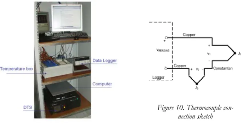
Figure 9. The data logging equipment
Figure 10. Thermocouple con-nection sketch
The description of the test installations in the following chapters include pictures of the borehole heat exchangers where the fiber optic cables can be observed after complete installation (see Figure 14, Figure 40, Figure 65, Figure 66). The laser generation and data acquisition system in all cases looks approximately like a normal computer, as shown in Figure 9. A tempera-ture box and a data logger is also part of the measurement instrumenta-tion. These are used in order to read local temperature at certain points
of interest by using thermocouples, the working principle of which is briefly illustrated by the sketch in Figure 10. Through the temperature box, each of the thermocouples is connected to a logger by a circuit with an internal reference temperature (J2). The measurement points in the BHE
are represented by the junction J1. The temperature is a function of the
voltage difference, which is read and interpreted by a logger.
The precision of a DTS measurement increases with the amount of in-formation read by the data acquisition instrument per unit time and with the size (length and diameter) of the observed section along the fiber, i.e. better accuracy is obtained when more photons are observed per unit time. However, the photon density decreases with increasing length of the measurement section, meaning that the amount of information read by the instrument in a certain period of time may also be smaller if the length of the observed section is large.
In this thesis, two different DTS instruments have been used: Sentinel and Halon, both from Sensornet and with spatial resolution of one and two meters, respectively. The spatial resolution is the maximum width of a step temperature change that the instrument can detect, and it is de-fined as the distance between 10% and 90% limits of a detectable tem-perature step. The instrument integrates (sums up) the signals from this section and determines an average temperature for this length. In case there is step temperature change, e.g. a hot or cold spot in the fiber ca-ble, the width of which is lower than the instruments spatial resolution, the measured temperature is affected by a factor approximately propor-tional to the ratio between the spot width and the spatial resolution. Moreover, the light signal becomes exponentially weaker as it travels through the fiber, meaning that the amount of information coming back to the DTS instrument decreases with the distance at which a measure-ment is to be taken, i.e. a section of the fiber located far away from the instrument needs a longer integration time. As a conclusion, for a given fiber optic cable, the expected precisions for temperature, time, and space, must be compromised in order to achieve the desired measure-ment quality.
The intensity of the laser is diverse for different DTS instruments and the fiber characteristics change manufacturer to manufacturer. In order to guarantee quality on distributed temperature measurements, a careful calibration process must be carried out. This normally requires the ad-justment of an offset and a slope correction during the calibration process in order to compensate for the losses along the cable length. Since the Borehole Heat Exchanger research installations in this thesis demanded special installation procedures and subsequent fiber and
con-nector splicing, the calibration process has been carried out after the bo-rehole heat exchanger installation and instrumentation was done, nor-mally under undisturbed ground temperatures conditions. This post-installation calibration process have consisted of placing two relatively long cable sections (separated from each other as much as possible) into one or even two environments with a known temperature such as an ice bath, by rolling together several meters of cable normally located before and after the borehole loop, as illustrated in Figure 11. The ice-bath ar-rangement was also insulated on the top.
Figure 11. Ice bath for fiber optic calibration
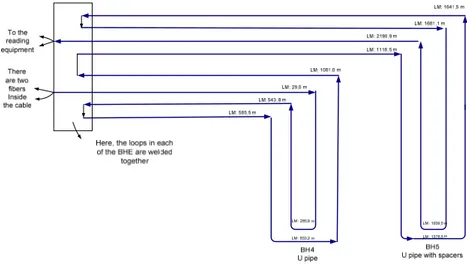
Figure 12 illustrates, as an example, the fiber cable loop from one of the re-search installations studied in this thesis. In this case, two BHEs are in-strumented with this technology and a common box is used to weld the different loops so that simultaneous measurements in both boreholes is possible.
Figure 12. Sketch of the fiber optic loop in two BHEs
The box where the loops are welded together in Figure 12 is, in this case, the link between the whole cable measurement length and the integration instrument (DTS shown in Figure 9). The numbers denoted with the tag LM:X are marks that delimit the beginning, bottom, and end of a certain