Application of some statistical methods for evaluation of groundwater observations

(1)

With the objective of reviewing different statistical methods for evaluation of groundwater data and the design of a groundwater observation network, a comprehensive literature survey was performed. The literature survey focuses on spatial statistics (geostatistics) but also includes methods to evaluate time-series of groundwater data and the determination of the sampling frequency. A method is developed which provides a means of quantifying the accuracy of an existing groundwater monitoring network with regards to spatial interpolation and the locations of the corresponding observation points. The spatial interpolation method of ordinary kriging was used. A result from ordinary kriging was estimated (interpolated) levels at unmeasured points, but also a kriging variance. The kriging variance can be interpreted as a measure of the estimation accuracy and used as a criterion for network design. Design of a monitoring network for groundwater levels in an area includes the selection of:

- the number of observation points and - the spatial locations of observation points.

The method was applied to design a monitoring network in an area in a glaciofluvial deposit, the Nybro esker, which is the main aquifer for the water supply of the Kalmar-Nybro region in the southeast of Sweden. This thesis shows that it is possible to quantify the accuracy of an existing observation network using the average kriging variance as a measure of accuracy. It is also possible to describe how this kriging variance changes (increases) when the observation network is reduced. By using this variance is it possible to rank the different points in the network as to their relative importance. It is thus possible to identify the points, which are to be removed when the observation network is reduced, one point at a time. This study shows that a monitoring network in the study area could be reduced by 35% while the increase in average estimation (kriging) variance is only about 10%. Although the method is applied to groundwater levels in a glaciofluvial deposit, it is applicable also to other variables that can be considered regionalized and to other geological environments.

(3)

Foreword

At the start of this licentiate project (Nov. 1997) the aim of the project was not clear. My first thoughts were to investigate methods to evaluate time-series of groundwater level observations and especially to find methods to detect the impact on groundwater systems from human activities. I had become aware of the usefulness of statistical methods to analyse time-series and to detect the effects of human impact. Dr Bo Olofsson, Royal Institute of Technology, who had done a great deal of research in this field brought this awareness to my attention. He also made me realise that it is of great importance how an observation program is designed, and that the observation program perhaps could be designed in an optimal way with the use of statistical methods. Another reason to focus on time-series was that I had access to a great number of observations from the Nybro esker, where groundwater levels have been observed and recorded since 1956.

My first attempt was to evaluate a time series of level observations from the Nybro esker and to make a time-series model. This model can be used to predict future observations and perhaps, used to detect an impact on the groundwater system. However, this study is not included in my thesis.

When I started to search in databases my focus was on statistical methods in both the temporal and the spatial domain which led me into the exciting field of geostatistics. Since geostatistical methods are primarily used for interpolation of data I found many scientific articles on this issue. But I had also began to think more in general, about how observation programs are designed initially, and after which criteria they are changed over time. Figure 1 is a result from this and describes in a simple way the different activities from the formulation of the objectives of observations to the results. From the data base search I also found several scientific articles describing the use of geostatistical methods for the design of monitoring networks. I thought that it was a nice symmetry to use the same tools to design a network as to evaluate the observations. I hereafter decided to go deeper into this concept and my case study deals with this problem. Another attempt to investigate statistical methods was when I evaluated a screening of groundwater constituents from Stockholm (Ackerberg 1999). The screening was performed by The Swedish Geological Survey (SGU) and they also supplied me with data. Because of the great number of variables, around 30, the study required the use of multivariate technique. I used Principal Component Analysis (PCA) and although the method of PCA, strictly speaking, is not a geostatistical method, the results from it can be given a spatial interpretation.

The thesis is based on the following parts, which are referred to in the text by their respective number.

Part 1. A literature review, “Application of some statistical methods for evaluation of groundwater observations.”

Part 2. A case study, ”Geostatistical design of a monitoring network for groundwater levels in a glaciofluvial deposit in southeastern Sweden”, and

Part 3. Appendices:

-Appendix One, Geological and hydrogeological description of the Nybro esker. -Appendix Two, MATLAB programs for solution of kriging equations.

(4)

Introduction

In areas where groundwater for consumption is being abstracted, it is usually stipulated that continuous observations regarding the groundwater quantity and quality must be made. Observations and evaluation of the observations are costly, so it is of vital importance to make the observation program as optimal as possible.

Optimisation of an observation network means that the total number of observations over a period of time is minimised while the objectives of the monitoring are fulfilled.

Before a groundwater resource (aquifer) can be used for abstraction, the geologic formation from which the groundwater is supposed to be abstracted, must be investigated. Relevant questions to be answered are:

- is this geologic formation valuable as a groundwater resource in the area of interest? - which are the potential areas for location of abstraction wells and infiltration basins? - where are the best locations for these wells and infiltration basins?

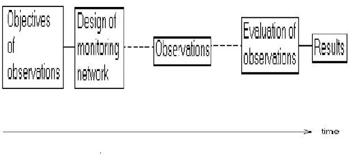
To answer these questions a number of boreholes are established to investigate the geologic and hydrogeologic properties of the geologic formation. In these boreholes, tubes or pipes for observations of groundwater levels and groundwater quality are installed. It is also possible to use dug wells for these observations. Thus an observation network is established in the formation, which can be used for continuous observations of groundwater quantity and quality. The different activities associated with the observations are shown in Figure 1 below.

Figure 1. Activities from the formulation of the objectives of observations to the results.

The observations are performed as point measurements, but since the observed variable almost always has a distribution in space there is therefore need during the evaluation of the observations to make estimates of the observed variable at locations where no observations have been made for example when mapping a variable over an area.

(5)

All estimates however have a certain degree of uncertainty which is important to estimate. One way to determine the quality of an estimate is to compare the estimated value with a measured value at the same point. The difference between the estimated and the measured value is an indicator of how good the estimate is. By repeating this procedure for a great number of points it is possible to determine the ability of an estimation method. When observed data is sparse such a procedure is not possible to follow, and there is a need for using some interpolation method that can produce a measure of the estimation accuracy without measured data to compare with. During the first period of time the total number of observation points in the network will increase as additional observation points are established, and this will continue until the network has reached its maximum. After some time, perhaps several years, the observation program usually must be reduced. The reason for such a reduction could be:

- less need for additional information - budget restrictions

- lack of competent personal to perform and evaluate investigations

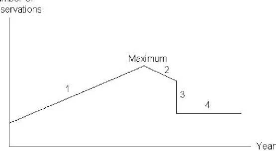
In a situation as the one described above, the total annual number of groundwater observations may vary over time as shown in Figure 2 below.

Figure 2. A graph, which describes how the total annual number of groundwater observations usually changes over time.

The meaning of Figure 2 is that when there is little knowledge about a geological formation, there is a need for an observation program. This program is successively extended until it reaches its maximum level and there is no need for additional observation points. This is symbolised by line 1 in the figure. From this maximum level a number of observation points are excluded from the network and the reasons for this may be:

- wells or tubes have dried out

- tubes have disappeared or are difficult to find

(6)

This reduction of the network is symbolised by line 2.

After some years a certain evaluation is performed in order to reduce the number of observation points according to the reasons previously mentioned. Removing one or several observation points at a time from the network would reduce the observation program. It is important to decide which points are to be removed without losing too much information. This reduction is symbolised by the line 3 and thereafter the number of observations follows line 4.

To reduce an observation network consisting of (n) points by one point, Cressie, (1993 p268) writes that one strategy is to delete the point that could be best predicted from the remaining (n-1) points.

Problems

A number of problems have thus been identified, and as far as estimation is concerned there are two issues that often must be addressed, these are:

- Which interpolation (estimation) method is the best regarding the monitoring objectives and considering the fact that, in the case of an existing observation network, that the number of observed data are sparse?

- Are there any interpolation methods which are able to produce some measure of the estimation accuracy together with the interpolated (estimated) value?

Concerning the problem of network design the following four issues, partially overlapping each other need to be addressed:

- How many observation points are needed, and which are the preferable spatial locations of these points to meet the monitoring objectives?

- How to determine an observation frequency to meet the monitoring objectives.

- How to define a simple criterion, for example the estimation accuracy, to be used when an observation program is to be reduced, or when it is developed.

- How to rank the different observation points in a network and to use this ranking when an observation network is being reduced i.e. points with the lowest rank are to be deleted from the network

Objectives and delimitations

The objectives of this thesis are twofold: 1. To review the literature regarding:

• different interpolation (estimation) methods for groundwater data (levels and chemical data).

• interpolation methods which have the ability to produce a measure of accuracy of the

estimated variable value.

• different approaches to design observation networks, i.e. determination of the number of

(7)

• the evaluation of groundwater times-series.

• methods to determine the sampling frequency for groundwater data as a part of observation

network design.

2. To develop, by means of a case study, a method to reduce the number of observation points in an existing network according to some well defined and simple criteria, and to rank the relative importance of the different points in the network.

The case study is limited to the spatial domain, and it only covers with groundwater levels.

Methods and materials

The first objectives were achieved by a literature review based on different: - Scientific articles

- Conference papers - Dissertations - Books

This material was obtained from libraries and databases such as: - Agricola

- Applied Science and Technology - BYGGDOK

- Compendex Web

- Conference Papers Index - Dissertation Abstracts - Geobase - Georef - MathSciNet - NTIS - Pascal

From the literature review the method of ordinary kriging was selected to design an observation network for groundwater levels. Ordinary kriging is an interpolation method, which has the advantage of producing a value of the interpolation error (the kriging variance) along with each interpolated variable value. The interpolation error can be interpreted as a measure of the interpolation accuracy, and the mean interpolation error over an area can be used as an objective function to design an observation network in the area.

The second objective was reached by a case study based on groundwater level observations from the Nybro esker. A more detailed data description can be found in the case study (part 2).

Although the method of ordinary kriging can be used to create new networks as well as for expansion or reduction of existing networks, it was in the case study used to reduce an existing observation network of groundwater levels.

To use the method of ordinary kriging as described above implies a great deal of numerical calculations. Computer software was therefore needed to solve the kriging equations (see part 1, section 6) and to study the effects of addition or deletion of a point from a network (see part 2, p 11-12). Since no appropriate software could be found in the literature to deal with the stated problems, the author developed a number of MATLAB programs. These programs were used for:

(8)

-estimation of variable values at unmeasured points, and calculation of the kriging variance

-cross-validation of a spatial model

-calculation of the effects on the average kriging variance, when observation points are deleted from a network.

These MATLAB programs are presented in part 3, Appendix Two.

Results and discussion

Several interpolation methods were examined in the literature review. Isaaks and Srivastava (1989 pp 313-320) compare different interpolation methods and they conclude that ordinary kriging performed slightly better than four other commonly used methods, namely triangulation, local sample mean, polygonal and inverse distance squared. It is however impossible to state that ordinary kriging in general is the best interpolation method (Gambolati and Volpi 1979b).

Furthermore, ordinary kriging has an important property which is the ability to produce a measure of accuracy, the kriging variance, along with the estimated value. Since this measure of accuracy (the kriging variance) depends on the number and locations of the observation points, it can be used to design observation networks in the spatial domain (Cressie 1993 p 314, Kitanidis 1997 p 78). Many authors (e.g. Delhomme 1978, Hughes and Lettenmaier 1981) have described this methodology and practical application.

The method of ordinary kriging is a comparatively simple method and it uses only measured variable values, for example groundwater levels, in an area. Since there is only one variable to model, this model (the variogram) is also simple and is preferable to use when the total number of data in an area is sparse (Kitanidis 1997). Because of its simplicity the method of ordinary kriging has advantages compared to more complex methods, such as Kalman filtering that uses a deterministic model to simulate the groundwater flow and has a great number of model parameters which must be calibrated. Much more data is thus required when the method of Kalman filtering is used (van Geer 1987).

To investigate time-series of groundwater level observations Law (1974) plotted groundwater level observations versus time and detected linear trends, jump trends, non-linear trends and periodic (seasonal) behaviour of the observations. These deterministic components were modelled and removed from the time series. The residuals were considered stochastic and analysed to find their probability density function.

The residuals can be considered the outcome of a stochastic process, which can be used as a model. The author tested stochastic modelling of groundwater time-series from the Nybro esker. These models were used to predict future groundwater observations. Since the model is built on historical data that reflects natural hydrological processes, any deviation in the future from the model predictions may indicate an anthropogenic impact.

Depending on the objective of the observations a sampling frequency (time lag between the observations) can be determined. In the case of multiple objectives (trend detectability estimation of periodic fluctuations and mean values) each yielding different sampling frequencies, the one with smallest time lag between observations must be chosen (Zhou 1996).

(9)

To be able to discover a periodicity of a time series, the observation frequency must be less than half of the periodicity. To determine a periodic component of, for example 6 months, an observation frequency of less than 3 months is required (Gunneson 1968).

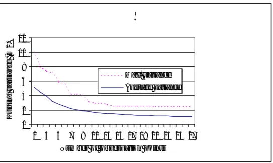
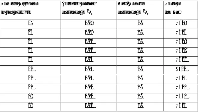
A special case of network design is when an existing observation network has to be reduced. In the case study (part 2) a method is developed where the observation points in the study area are ranked, and the relative importance for each point in the network assessed. When the network is to be reduced by one point, the least important point, i.e. the one with the lowest ranking, is removed. The least important point is the one which causes the minimum increase of the average kriging variance over the area when removed from the network. By successively removing points from the network and calculating the average kriging variance, a Network Density Graph (NDG) showing the average kriging variance as a function of the number of observation points can be generated (Figure 3). I table 1 these points are listed in the order they are removed from the network together with the corresponding average kriging variance for the network. With Figure 3 and Table 1 is it, according to an a´-priori acceptable kriging variance, possible to determine both the total number of observation points, and which points that are to be included in the network.

If, for example, an average kriging variance of 1.12 m2_{is required, the total number of}

observation points is 24, and the points to be removed from the network are U329, U326 and U328.

This study shows that a monitoring network in the study area could be reduced by 35% while the corresponding increase in average estimation (kriging) variance is only about 10%.

Figure 3. Network Density Graph of the study area showing the average and maximum kriging variance as a function of the number of observation points.

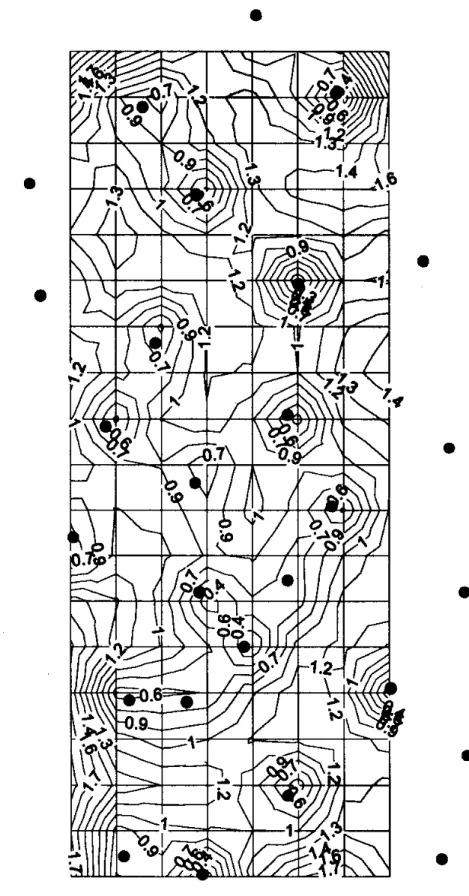
A map showing the variation of the interpolation error (kriging variance) over the area for a certain number of observation points can also be calculated. Figure 4 shows the variation of the interpolation error for a network of 27 observation points.

As stated above the Network Density Graph (NDG) is used to describe the relationship between the kriging variance and the number of observation points. In previous works this method have been used by Ting et al. (1997a) and also Van Bracht and Romjin (1985). They, however,

0 2 4 6 8 10 12 1 3 5 7 9 11 13 15 17 19 21 23 25 27

Number of observation points

Kriging variance (m

2)

Max. variance Average variance

(10)

calculated the NDG based on synthetic observation points in a regular pattern with different grid spacing. A NDG of that kind could only be used to determine the number of points in a network for an a´-priori kriging variance.

Table 1. Shows the order in which the first 10 points are to be removed from an existing observation network, and the kriging variance associated with each number of observation points. The complete table can be seen in part 2 page 19.

Number of points Average kriging Max. kriging Point to in the network variance (m2) variance (m2) remove

27 1.09 2.5 U329 26 1.09 2.5 U326 25 1.10 2.5 U328 24 1.12 2.5 U327 23 1.14 2.5 U322 22 1.16 2.5 B321 21 1.16 2.5 U313 20 1.22 2.6 U321 19 1.22 2.6 U330 18 1.22 2.6 U325

(11)

(12)

Conclusions

The main conclusions from this thesis are that:

- ordinary kriging is an interpolation method that has the desired property of producing a measure of accuracy (a kriging variance), together with the estimated variable value.

- this kriging variance is useful when an existing observation network has to be reduced.

- it is possible to rank the importance of the different points in an observation network, and that this ranking can be used when reducing a network is by removing points with low ranking.

- the case study shows that a monitoring network in the study area could be reduced by 35% while the increase in average estimation (kriging) variance is only about 10%.

Future Perspectives

The present case study dealt with data in the spatial domain only. This means that the sampling frequency was not included although a method to account for this has been described in the literature review. An interesting approach well worth to investigate is to apply a geostatistical method (kriging) also to the time domain. A temporal variogram valid for several observation points in a particular area could be calculated. Together with the spatial variogram it is perhaps possible to interpolate first in the spatial, and then in the temporal domain. A kriging variance, as a measure of the interpolation accuracy could be calculated for both the spatial and temporal cases and then combined as a total kriging variance. This total variance could then be used in the same way as described in the spatial domain. This makes it possible to analyse different numbers and locations of observation points as well as the corresponding sampling frequency.

Acknowledgements

Thanks to my supervisors Prof. Roger Thunvik and Prof. Gert Knutsson at the Department of Land and Water Resources Engineering, Royal Institute of Technology.

Thanks to Sigbert Rickardsson for interesting discussions concerning the Nybro esker

and to Ingvar Haglund for his help to acquire data, both at Kalmar municipal, Water and Waste company.

Thanks also to Lars Kylefors at Vatten and Samhällsteknik Ltd.

Special thanks to Sven Follin for very interesting discussions concerning Geostatistics and to Craig McConnachie for lingvistic revision.

Thanks to Gerhard Barmen who led the licentiate seminar and to my Nybro esker partner, Åse Eliasson.

(13)

References

Ackerberg, Björn. 1999. Multivariate analysis of groundwater chemical constituents. Technical report, Department of Land and Water Resources, KTH, Stockholm. In Swedish. Cressie, N.A.C. 1993. Statistics for spatial data. John Wiley and sons Inc. ISBN 0-471-00255-0.

Delhomme, J. P.; 1978. Kriging in the hydrosciences. Advances in Water Resources, 1 pp251-266.

Gambolati, G.; Volpi,G. 1979. A conceptual deterministic analysis of the kriging technique in hydrology. Water Resources Research 15(3) , pp625-629. June 1979.

Gunnerson, C.G. 1968 Optimizing Sampling Intervals. Proceedings IBM Scientific Computing Symposium. Water and Air Resource Management , White Plains, N.Y. , pp 115-140.

Hughes, James P.; Lettenmaier, Dennis P. 1981. Data Requirements for Kriging: Estimation and Network Design. Water Resources Research. Vol 17, no 6, pp 1641-1650.

Isaaks, Edward A.; Srivastava, Mohan, R. 1989. An Introduction to Applied Geostatistics. Oxford University Press.ISBN 0-19-505013-4.

Kitanidis, P.K. 1997. Introduction to Geostatistics, applications in hydrogeology. Cambridge University Press. ISBN 0-521-58747-6.

Law, Albert G. Stochastic analysis of groundwater level Time Series in the Western United States. Colorado State University (Fort Collins), Hydrology Papers n68 May 1974. 26p.

Ting, Cheh-Shyh; Liu, Chen W.; Tsai, Wei-Wen. 1997a. Application of geostatistical analysis in the design of a groundwater level monitoring network for Pingtun Plain, Taiwan: 1. Network density. Proceedings,Congress of the International Assosiation of Hydraulic Research, IAHR. Part C Aug 10-15 pp27-33.

van Bracht, M. J.; Romijn, E. 1985. Redesign of Groundwater Level Monitoring Networks by Application of Kalman Filter and Kriging. Proceedings of the Symposium of the Stochastic Approach to Subsurface Flow, Montvillargenne, France, pp117-127.

van Geer, F.C. 1987. Applications of Kalman filtering in the analysis and design of groundwater monitoring networks, report, Delft University of Technology, Delft Nederlands, 1987.

Zhou, Yangxiao. 1996. Sampling frequency for monitoring the actual state of groundwater systems. Journal of Hydrology. May 15 1996 pp301-318.