A performance measurement of a Speaker Verification system based on a variance in data collection for Gaussian Mixture Model and Universal Background Model

Faculty of Technology and Society

Department of Computer Science and Media Technology

Master Thesis Project, Spring 2018

A performance measurement of a Speaker

Verification system based on a variance in data

collection for Gaussian Mixture Model and

Universal Background Model

By

B.S.E. in Computer Engineering Zeid Bekli

B.S.E.in Computer Engineering William Ouda

Supervisors:

Arezoo Sarkheyli Haegele

Examiner:

Johan Holmgren

Contact information

Authors:

Supervisor:

Arezoo Sarkheyli Haegele

E-mail: arezoo.sarkheyli-haegele@mah.se

Malmö University, Department of Computer Science and Media Technology.

Examiner:

Johan Holmgren

E-mail: johan.holmgren@mau.se

i

Abstract

Voice recognition has become a more focused and researched field in the last century, and new techniques to identify speech has been introduced. A part of voice recognition is speaker verification which is divided into Front-end and Back-end. The first component is the front-end or feature extraction where techniques such as Mel-Frequency Cepstrum Coefficients (MFCC) is used to extract the speaker specific features of a speech signal, MFCC is mostly used because it is based on the known variations of the humans ear’s critical frequency bandwidth. The second component is the back-end and handles the speaker modeling. The back-end is based on the Gaussian Mixture Model (GMM) and Gaussian Mixture Model-Universal Background Model (GMM-UBM) methods for enrollment and verification of the specific speaker. In addition, normalization techniques such as Cepstral Means Subtraction (CMS) and feature warping is also used for robustness against noise and distortion. In this paper, we are going to build a speaker verification system and experiment with a variance in the amount of training data for the true speaker model, and to evaluate the system performance. And further investigate the area of security in a speaker verification system then two methods are compared (GMM and GMM-UBM) to experiment on which is more secure depending on the amount of training data available.

This research will therefore give a contribution to how much data is really necessary for a secure system where the False Positive is as close to zero as possible, how will the amount of training data affect the False Negative (FN), and how does this differ between GMM and GMM-UBM.

The result shows that an increase in speaker specific training data will increase the performance of the system. However, too much training data has been proven to be unnecessary because the performance of the system will eventually reach its highest point and in this case it was around 48 min of data, and the results also show that the GMM-UBM model containing 48- to 60 minutes outperformed the GMM models.

Keywords: Speaker recognition; Speaker Verification; Speaker authentication; Speaker classification Text-dependent; Text-independent; Gaussian mixture model; Gaussian Mixture Model-Universal Background Model; Biometric System; Equal Error Rate; False Negative Rate; False Positive Rate; Mel Frequency Cepstrum Coefficients;

ii

Acknowledgement

We would like to show our appreciation to our supervisors Christoffer Cronström, Niklas Hjern and Arezoo Sarkheyli Haegele for taking the time to guide and support us during this thesis.

iii Table of contents 1. Introduction ... 1 1.1 Research Motivation ... 3 1.2 Research Question ... 4 1.3 Limitation ... 4 2. Theoretical Background ... 6 2.1 Biometrics System ... 6 2.1.1 Verification System ... 7 2.1.2 Identification System ... 7

2.1.3 Speaker Verification System ... 8

2.1.4 Performance Metrics for Biometric Systems ... 8

2.2 Digital Signal Processing ... 9

2.2.1 Frame-Blocking and Frame-Overlapping ... 9

2.2.2 Hamming Window ... 9

2.2.3 Discrete Fourier Transform ... 10

2.2.4 Spectrum ... 10

2.2.5 Cepstrum ... 10

2.2.6 Mel-Frequency Cepstrum Coefficients ... 10

2.3 Speech Signals ... 11

2.4 Voice Modeling ... 11

2.4.1 Gaussian Mixture Model ... 12

2.4.2 Universal Background Model ... 13

3. Related Work ... 15

3.1 Hossan. M.A., et al. - A Novel Approach for MFCC Feature Extraction... 15

3.2 Fang, Z., et al. - Comparison of Different Implementations of MFCC ... 16

3.3 Chao-Yu, L., et al. - User Identification Design by Fusion of Face Recognition and Speaker Recognition ... 16

3.4 Mohamed, K.O., et al. - Training Universal Background Models for Speaker Recognition ... 17

3.5 Taufiq, H., et al. - A Study on Universal Background Model Training in Speaker Verification ... 18

3.6 Pelecanos, J., et al. - Feature Warping for Robust Speaker Verification ... 19

3.7 Kumari, T. J., et al. - Comparison of LPCC and MFCC features and GMM and GMM-UBM modeling for limited data speaker verification ... 20

4. Method ... 21

4.1 Construct a Conceptual Framework ... 22

iv

4.3 Analyze and Design the System ... 23

4.4 Build the (prototype) System ... 24

4.5 Observe and Evaluate the System ... 24

5. Results ... 25

5.1 The System ... 25

5.2 The Feature Extraction Phase ... 26

5.2.1 Mel-Frequency Cepstrum Coefficients ... 26

5.2.1.1 Sampling ... 26

5.2.1.2 Pre-Emphasis ... 26

5.2.1.3 Frame Blocking ... 29

5.2.1.4 Hamming Window ... 29

5.2.1.5 Discrete Fourier Transform ... 30

5.2.1.6 Mel-Filterbank ... 31

5.2.1.7 Discrete Cosine Transform ... 32

5.2.2 Normalization and Derivatives ... 33

5.3 The Enrollment Phase ... 35

5.4 The Verification Phase ... 35

5.5 Results ... 36

5.5.1 The GMM-UBM Method ... 37

5.5.2 The GMM Method ... 43

5.6 Analysis ... 49

6 Discussion ... 52

6.1 Method Discussion ... 52

6.2 The Speaker Verification System Components ... 52

6.3 Speaker Verification System Performance ... 53

7 Conclusion ... 55

7.1 Answering the Research Question ... 55

7.1.1 How does the GMM-UBM speaker verification system perform based on different amount of data collection for the true speaker model? ... 55

7.1.2 How does the GMM speaker verification system perform compared to the GMM-UBM, based on different amount of data collection for the true speaker model? ... 56

7.2 Further Work ... 56

7.3 Contribution of this Thesis ... 56

v

LIST OF FIGURES

FIGURE 1:THE OPERATIONS OF A TYPICAL BIOMETRIC SYSTEM [1] ... 6

FIGURE 2:THE VERIFICATION PROCESS ... 7

FIGURE 3:IDENTIFICATION PHASE WITH A SET OF SPEAKERS ... 7

FIGURE 4:EER METRIC STRUCTURE [40] ... 8

FIGURE 5: BLOCK DIAGRAM OF MFCC WITH DELTA AND DELTA-DELTA ... 11

FIGURE 6:THE PROCESS OF THE GMM-UBM ... 14

FIGURE 7:SYSTEMS DEVELOPMENT RESEARCH METHODOLOGY[33] ... 21

FIGURE 8:A COMMON SYSTEM ARCHITECTURE FOR SPEAKER VERIFICATION ... 22

FIGURE 9: SYSTEM ARCHITECTURE AND COMPONENTS FOR A SPEAKER VERIFICATION SYSTEM[34] ... 23

FIGURE 10:THE THREE MAIN COMPONENTS FOR A SPEAKER VERIFICATION SYSTEM ... 25

FIGURE 11A:ORIGINAL SIGNAL ... 27

FIGURE 11B:PRE-EMPHASIS SIGNAL ... 27

FIGURE 11C:ORIGINAL SIGNAL (PS) ... 28

FIGURE 11D:PRE-EMPHASIS SIGNAL (PS) ... 28

FIGURE 12A:A FRAME FROM THE SPEECH SIGNAL ... 29

FIGURE 12B:HAMMING WINDOW ON THE FRAME ... 30

FIGURE 13A:THE FILTER BANK WITH 32 FILTERS ... 31

FIGURE 13B:THE ENERGIES EXTRACTED FROM A SINGLE FRAME ... 32

FIGURE 14A:ORIGINAL DISTRIBUTION OF COEFFICIENT ... 33

FIGURE 14B:NORMALIZED DISTRIBUTION OF COEFFICIENT ... 34

FIGURE 15A:SHOWS THE SCORE DISTRIBUTION FOR MODEL ONE BETWEEN THE TRUE SPEAKER AND IMPOSTER SPEAKER (SPEAKER ONE). ... 39

FIGURE 15B:SHOWS THE SCORE DISTRIBUTION FOR MODEL EIGHT BETWEEN THE TRUE SPEAKER AND IMPOSTER SPEAKER (SPEAKER TWO). ... 39

FIGURE 15C:SHOWS THE SCORE DISTRIBUTION FOR MODEL ONE BETWEEN THE TRUE SPEAKER AND IMPOSTER SPEAKER (SPEAKER TWO). ... 40

FIGURE 15D:SHOWS THE SCORE DISTRIBUTION FOR MODEL EIGHT BETWEEN THE TRUE SPEAKER AND IMPOSTER SPEAKER (SPEAKER TWO). ... 40

FIGURE 16A:SHOWS THE DET CURVE FOR MODEL ONE (SPEAKER ONE). ... 41

FIGURE 16B:SHOWS THE DET CURVE FOR MODEL EIGHT (SPEAKER ONE). ... 41

FIGURE 16C:SHOWS THE DET CURVE FOR MODEL ONE (SPEAKER TWO). ... 42

FIGURE 16D:SHOWS THE DET CURVE FOR MODEL EIGHT (SPEAKER TWO). ... 42

FIGURE 17A:SHOWS THE SCORE DISTRIBUTION FOR MODEL ONE BETWEEN THE TRUE SPEAKER AND IMPOSTER SPEAKER (SPEAKER ONE). ... 45

FIGURE 17B:SHOWS THE SCORE DISTRIBUTION FOR MODEL EIGHT BETWEEN THE TRUE SPEAKER AND IMPOSTER SPEAKER (SPEAKER ONE). ... 45

vi

FIGURE 17C:SHOWS THE SCORE DISTRIBUTION FOR MODEL ONE BETWEEN THE TRUE SPEAKER AND IMPOSTER

SPEAKER(SPEAKER TWO). ... 46

FIGURE 17D:SHOWS THE SCORE DISTRIBUTION FOR MODEL EIGHT BETWEEN THE TRUE SPEAKER AND IMPOSTER SPEAKER (SPEAKER TWO). ... 46

FIGURE 18A:SHOWS THE DET CURVE FOR MODEL ONE (SPEAKER ONE). ... 47

FIGURE 18B:SHOWS THE DET CURVE FOR MODEL EIGHT (SPEAKER ONE). ... 47

FIGURE 18C:SHOWS THE DET CURVE FOR MODEL ONE (SPEAKER TWO). ... 48

FIGURE 18D:SHOWS THE DET CURVE FOR MODEL EIGHT(SPEAKER TWO). ... 48

FIGURE 19A:THE EER FOR THE EIGHT MODELS FOR GMM AND GMM-UBM(SPEAKER ONE). ... 50

FIGURE 19A:THE EER FOR THE EIGHT MODELS FOR GMM AND GMM-UBM(SPEAKER TWO). ... 50

FIGURE 20A:THE FN FOR THE EIGHT MODELS FOR GMM AND GMM-UBM(SPEAKER ONE). ... 50

vii LIST OF TABLES

TABLE 1:THE MAIN CONTRIBUTION OF THIS RESEARCH COMPARED TO RELATED WORK ... 4

TABLE 2:RESULTS FOR SPEAKER ONE BASED ON EIGHT MODELS WITH DIFFERENT AMOUNT TRAINING DATA WITH GMM-UMB MODELING. ... 37

TABLE 3:RESULTS FOR SPEAKER TWO BASED ON EIGHT MODELS WITH DIFFERENT AMOUNT TRAINING DATA WITH GMM-UMB MODELLING. ... 38

TABLE 4:RESULTS FOR SPEAKER ONE BASED ON EIGHT MODELS WITH DIFFERENT AMOUNT TRAINING DATA WITH GMM MODELING. ... 43

TABLE 5:RESULTS FOR SPEAKER ONE BASED ON EIGHT MODELS WITH DIFFERENT AMOUNT TRAINING DATA WITH GMM MODELING. ... 44

viii List of acronyms

CMS Cepstral Means Subtraction

DCT Discrete Cosine Transform

DET Detection Error Trade-off

DFT Discrete Fourier Transform

EER Equal Error Rate

EM Expectation Maximization

FFT Fast Fourier Transform

FIR Finite Impulse Response

FN False Negative

FNR False Negative Rate

FP False Positive

FPR False Positive Rate

GMM Gaussian Mixture Model

GMM-UBM Gaussian Mixture Model-Universal Background Model

GMM SVM Gaussian Mixture Model Support Vector Machine

HMM Hidden Markov Model

IDFT Inverse Discrete Fourier Transform

LPC Linear Prediction Coding

LPCC Linear Predictive Cepstral Coefficients

MAP Maximum a Posteriori

MFCC Mel-Frequency Cepstrum Coefficients

NPC Neural Predictive Coding

PLP Perceptual Linear Prediction

PS Power Spectrum

SVM Support Vector Machine

ix

1

1. Introduction

Recognition of body, face and voice has been utilized by humans for thousands of years to recognize other humans and objects. This is an ability that humans have from a young age to distinguish a mother, father, etc. [1][2]. There are a few occasions where one can be deceived by appearance, e.g. similar dressing, colors and so on [1]. Recognition in a larger scale can be difficult for human perception, and therefore it could help to find a way to automate this recognition, and the automated recognition of individuals based on biological characteristics is referred as biometrics [1].

A biometric system is an automated pattern recognition system [2], the operations of such a system is to capture biometric samples such as voice, face, fingerprints, etc. and compare them to already collected biometric reference samples that are already enrolled. The biometric system is then able to match the samples depending on different models and algorithms [1]. To further understand the biometric system functionality, it is best described through an illustration in figure 1.

The progress in digital electronics with the development of new algorithms and computing hardware has made it possible for people to utilize voice-based applications. The advantage of speech is to be able to express something, communicate and interact. A Speech signal consists of a sequence of sound waves, this sequence is formed through acoustical excitation of the vocal tract (comprising the throat, mouth and nasal cavity) when air is expelled from the lungs [3][4][5]. And with the development of voice-operated functions many high-tech products have been developed with biometric identification technology, e.g. Speech- and speaker recognition that utilizes speech signals to interact with TVs, smartphones, and home personal assistants, just to name a few. Controlling the lights in your home, setting alarms and locking the front door through your speech is possible with Amazon Echo and the recently launched Google Home in 2016 [6][7][8]. In most cases these devices are in a home environment and have control over things that need to be secure, and therefore a need for security technology has increased and has to be implemented. With security in focus then such technologies with Biometric recognition i.e. speaker recognition can be one solution [9][10].

2

To increase the recognition rate and security in the biometric system then a combination of biometric identification is possible e.g. combining face recognition and speaker recognition or speaker recognition with fingerprint recognition etc. The combined system is able to analyze and determine if the person is who he is claiming to be, if the system matches the person to the claimed identity, then person is the “client”. While if the system does not find a match in the system then that person will be regarded as an imposter [11]. Many applications today utilize voice recognition technology and depending on the nature of the application it is possible to see if the application is focused on speech

recognition or speaker recognition. Speech recognition is the ability to recognize words

from the human speech, while speaker recognition refers to the task of recognizing and identifying the person that is speaking based on the spoken utterance. Speaker recognition is then also divided into two parts, the first part is speaker identification and the second part is speaker verification. Speaker identification is to determine who is speaking based on a set of registered speakers, and speaker verification on the other hand is to analyze and then determine if the unknown voice is from the claimed speaker (true speaker1) [7][9][12]. The speaker recognition system can also be modeled to be either text-dependent or text-intext-dependent. A text-text-dependent system is based on the same utterance “specific password” from the claimed speaker. While for a text-independent system there is no such constraint, the system will recognize the specific speaker based on other utterances “passwords” [11].

The speaker verification system is divided into two phases, enrollment and verification. The enrollment phase is to capture biometric samples and compare them to already collected biometric reference samples as mentioned above, and typically a feature extraction method is required such as Mel Frequency Cepstral Coefficients (MFCC) to extract the specific speakers features. The MFCC features can also be used for a text-independent system. After that is the verification phase which is the part to recognize the specific speaker based on features extracted, and statistical approaches such as Gaussian Mixture Model (GMM), Gaussian Mixture Model-Universal Background Model (GMM-UBM), Gaussian Mixture Model Support Vector Machine (GMM-SVM) model, Hidden Markov Model (HMM) and neural networks are preferred for matching [11]. In recent years, approaches for text-independent verification systems are GMM based (e.g.

3

UBM, GMM-SVM) and has been almost exclusive [13]. HMM based approaches has not shown any advantages for speaker recognition systems that are text-independent compared to GMM based approaches [14].

“There is no concrete evidence that using the maximum amount of data would guarantee the best overall performance” [13]. Which in turn means that more training data would not necessarily give better performance because of the physical constraints of the humans that will limit the speech to only occupy a limited region in the feature space [13].

1.1 Research Motivation

The aim of this research is to investigate the performance of the true speaker data collection in a GMM-UBM based speaker verification system, the reason for this research is to conclude on how much data is necessary for the system, as Taufiq, H. et al. [13] said in his research that there is no concrete evidence that says that too much data is “always better”. This research will therefore give a contribution to how much data is necessary for a secure system where the False Positive is as close to zero as possible, how will the amount of training data affect the False Negative (FN). The main goal of this study is to provide the researchers with knowledge of how much training data is needed for a speaker verification system, this will save the researchers a lot of time and funds. To further investigate the area of security in a speaker verification system then two methods are compared (GMM and GMM-UBM) to experiment on which is more secure depending on the amount of training data available. This will help the researchers to choose the right method at an early stage depending on the system criterias they set up.

4 GMM compared to

GMM-UBM with true speaker model (data

less than 15 sec)

GMM-UBM imposter model (amount of data

needed)

GMM compared to GMM-UBM with true

speaker model (data between 45 sec to 1 hour) GMM-UBM true speaker model (amount of data between 45 sec to 1 hour) This Research X X Kumari, T. J., Jayanna H. S.[28] X Pelecanos, J. et al. [32] X

Table 1: The main contribution of this research compared to related work

The papers in chapter 3 are related to this thesis in many ways, e.g. how to extract features from an utterance or how the enrollment phase is set up and or algorithms for the verification phase, but considering the research question than two papers are highly related to this thesis and are therefore presented in Table 1.

1.2 Research Question

The aim of this research is to investigate the performance of the true speaker data collection in a biometric speaker verification system, and therefore propose this research questions below.

Research Question One: How does the GMM-UBM speaker verification system

perform based on different amount of data collected for the true speaker model?

Research Question Two: How does the GMM speaker verification system perform

compared to the GMM-UBM, based on different amount of data collected for the true speaker model?

1.3 Limitation

The limitations and approaches for handling threats to validity will be brought up in this section. The verification system is based on the program Matlab in a personal computer. In the enrollment phase the use of MFCC for feature extraction is used with GMM-UBM- and GMM models for the verification phase of the system. The imposter model contains two databases, one database contains approximately 5.4 hours of data and the other one around 1 hour of data which is in total around 6.4 hours of data that is used for training the imposter model. The imposter data consists of 70% male speakers and 30% female

5

speakers. The evaluation of the results in chapter 5.5 are based on 9 male- and 1 female speaker. The training of the imposter data is recorded with two different microphones for avoiding any biased results. One of these microphones was used when collecting true speaker data and evaluation data. Two true speakers (male) will be evaluated in sixteen models (eight for GMM classifier and eight for GMM-UBM classifier) each, and the amount of training data consist of 45 seconds up to 1 hour without any use of silence removal.

6

2. Theoretical Background

The aim of this chapter is to review the areas that are important to understand in order to follow the chapters ahead in this thesis. Each subsection below should give a sufficient understanding to each term.

2.1 Biometrics System

Biometric is the physical characteristics of a human being (e.g. voice, fingerprinting, face). A biometric system is a pattern recognition system that acquires biometric features from human beings, that are compared with the features stored in a database.

There is a variety of biometric characteristics systems used (e.g. DNA, face, fingerprint, signature, voice, iris, etc.) each has its strengths and weaknesses [2][15].

Figure 1: The operations of a typical biometric system [1]

The biometric system is divided into enrollment and verification. In the enrollment phase the system decides if the subject is existing in the system “database” and if not then the subject should be added for future reference. While in the verification phase the system compares the subject with existing references and returns a match if found [1].

7 2.1.1 Verification System

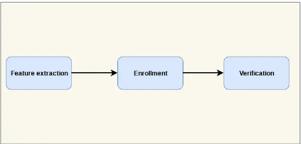
In the verification system, a person claims to be a certain user whose biometrics features are saved in a database. This is done by providing ID (can be PIN number, name, RFID tag etc.) then the model is retrieved from the database to be compared, if the claimed person is the intended user or an imposter. In this way, the system is validating the person's identity e.g. person one is the true speaker [2][16].

Figure 2: The verification process

2.1.2 Identification System

An Identification system operates to recognize an individual by searching the “database” of all the models of the users, and to find a match. This is the main difference between verification (one-to-one comparison) and identification (one-to-many comparison) [2][16].

8 2.1.3 Speaker Verification System

Speaker verification system can be divided into two modalities, text-independent and text-dependent. A text-independent identification system relies on the characteristics of the vocal tract of the speaker. This is a more complex modality which can offer better protection against imposters. A challenge of text-independent verification systems is that the features are more sensitive to background noise. While for text-dependent verification systems, they are dependent on a fixed phrase that is predetermined [2][16].

2.1.4 Performance Metrics for Biometric Systems

One popular performance metric in biometric systems is the Equal Error Rate (EER). Biometric systems have a trade off between False Negative Rate (FNR) and False Positive Rate (FPR) and the EER is a measure of the error rate of the system when the threshold is varied so that the number of FNR is equal to the number of FPR [16].

The Detection Error Trade-off (DET) curve was introduced by National Institute of Standard and Technology in 1997 and has been favored since then. The DET curve plots the percentage FNR on Y-axis versus percentage FPR on X-axis and the DET curve uses a logarithmic scale for plotting the two rates [2][16].

9

To calculate the FNR and FPR then these equations are as followed.

𝐹𝑁𝑅 = 𝐹𝑁/(𝐶𝑜𝑛𝑑𝑖𝑡𝑖𝑜𝑛 𝑃𝑜𝑠𝑖𝑡𝑖𝑣𝑒) = 𝐹𝑁/(𝐹𝑁 + 𝑇𝑃) (1) 𝐹𝑃𝑅 = 𝐹𝑃/(𝐶𝑜𝑛𝑑𝑖𝑡𝑖𝑜𝑛 𝑁𝑒𝑔𝑎𝑡𝑖𝑣𝑒) = 𝐹𝑃/(𝐹𝑃 + 𝑇𝑁) (2)

2.2 Digital Signal Processing

Signals are patterns of variations that represent information. There are all kinds of signals such as speech signals, audio signals, video or image signals, radar signals, just to name a few [17] [18].

Many signals originate as continuous-time signals, and speech signals are one of these. It can sometimes be desirable to obtain the discrete-time representation of the signal, and one way to do this is through sampling equally spaced points in time. The result will be a discrete time representation of the signal that can be processed digitally [17]. Digital Signal Processing (DSP) refers to a set of algorithms that are used to process digital signals, the usage for some of these algorithms is to improve the signal by using techniques such as Discrete Fourier Transform (DFT), Finite Impulse Response (FIR). Other algorithms that are used with DFT and FIR are Windowing [19].

2.2.1 Frame-Blocking and Frame-Overlapping

Frame-blocking is to split the signal into frame blocks, the frames are usually between 10 to 30 milliseconds. This is necessary in order to capture the local spectral properties that are assumed to be stationary. Then to smoothen the transition from one frame to the other, an overlapping technique is used [20].

2.2.2 Hamming Window

A hamming window is used on each frame of the signal. This is needed to remove or reduce any signal discontinuities at the start of the frame and at the end of the frame when doing Fourier analysis. For MFCC the most common window used is Hamming window, followed in equation 3 [2][16][21].

𝐹𝑘 = 0.53836 − 0.46164𝑐𝑜𝑠 ( 2𝜋𝑛

10 2.2.3 Discrete Fourier Transform

DFT is to transform a signal from time domain to frequency domain. This is done by taking a sequence of sampled data and compute the frequency content in it, e.g. extract the frequencies that the speech signal is composed of. This represent the frequency domain of the signal opposed to the time domain. This is a powerful tool in DSP applications, this allows an examination of the frequencies in any given signal [17][22]. The Fast Fourier Transform (FFT) is an optimized algorithm of the DFT [17][22][23].

2.2.4 Spectrum

The spectrum of a speech signal is referring to the frequencies that are extracted with a Fourier transformation on a single frame [20], this is a powerful tool which provides the spectral content of the speech signal. And with the Inverse Discrete Fourier Transform (IDFT) it is possible to go back to the time domain. Simply put, a plot of the time domain will reveal the changes that are occurring over time, while for the frequency domain it specifies how much of the signal is in a given frequency band over a range of frequencies [22][24].

2.2.5 Cepstrum

The cepstrum can be considered to be a spectrum of a spectrum, mathematically it is the IDFT of a logarithm of the magnitude of the DFT of the signal. Cepstrum is more preferred in this case instead of the regular spectrum because it has the ability to separate the spectral envelope and the excitation signal from the spectrum. The process is that when taking the IDFT of the spectrum a lower frequency “spectral envelope” and a higher frequency “excitation signal” will be extracted. The main reason for this is to “filter out” the higher frequencies and attain the vector of cepstrum coefficients [24].

2.2.6 Mel-Frequency Cepstrum Coefficients

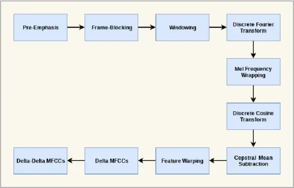
The MFCC method is widely used in Speaker verification systems. The aim of a feature extraction technique is to characterize an individual’s vocal tract information, and the MFCC is popular because it is based on the known variation of the human ear’s critical frequency bandwidth. In this paper the MFCC, Delta and Delta-Delta is built with the following blocks seen in figure 5 [25]

11

Figure 5: Block diagram of MFCC with Delta and Delta-Delta

2.3 Speech Signals

Speech is a tool humans use to communicate, and the speech signal is generated through the mouth when air is moving from the lungs to the throat and through the vocal tract. This tool is one way of expressing languages. And speech can be characterized in terms of signals carrying a message, which is the acoustic waveform [22]. Speech signals are based on the physical shape of the person, mouth, vocal tracts, age, medical conditions and emotional state. These conditions can change the speech signals over time [2].

2.4 Voice Modeling

There are two important parts in speaker recognition, the first part (front-end) which handles feature extraction that is to extract the features from a speech signal, and the second part (back-end) is the modeling and verification phase, this can be seen in figure 6. The most common modeling techniques used are HMM and GMM. The main difference to consider for the speaker verification system is that HMM is text-dependent and GMM is text-independent [24][26].

12 2.4.1 Gaussian Mixture Model

The GMM is a powerful tool for modeling text-independent system (has also been used in text-dependent systems). GMM is used in many applications that are involved with statistical data analysis, pattern recognition, computer vision, voice and image processing, and machine learning. The GMM is able to handle difficulties with data analysis and clustering with the finite mixture of gaussian densities. GMM handles clustering which is an unsupervised classification of data put into groups (clusters). This makes the GMM a useful probabilistic model for clustering of data, and current state-of-the-art text-independent GMM systems obtain the background model parameters by using the Expectation Maximization (EM) algorithm [21]. Example of application areas that utilize GMM is traffic surveillance, foreground segmentation, image coding, tracking and classifying activities, to name a few [24][27]. The mathematical form of GMM is seen in equation 4 below and is defined as a parametric probability density function and is represented as a weighted sum of M gaussian components [27][27][28].The advantage of the GMM method compared to the GMM-UBM is that it requires less training data for the imposter model, while a disadvantage is that it requires more training data for the true speaker model [28][29].

The GMM method is a likelihood function with a mixture of M Gaussians illustrated in the equations below [21].

𝑝(𝑥|𝜆) = ∑𝑀_𝑖=𝑖𝑤_𝑖𝑝_𝑖(𝑥)

x is a set of features (MFCCs), and 𝒑_𝒊(𝒙)is the individual Gaussian density function. The parameters for the model are the mixture weight 𝒘𝒊, the mean vector 𝜇_𝒊, and covariance matrix ∑.𝑖. which in short can be written as 𝜆= (𝑤𝑖, 𝜇_𝑖,∑.𝑖.) where i = [1...M].

𝑝_𝑖(𝑥) = 1 (2𝜋)𝑛/2_|∑. 𝑖|1/2 × 𝑒𝑥𝑝 {− 1 2(𝑥 − 𝜇𝑖) ′_{∑ (𝑥 − 𝜇} 𝑖) −1 𝑖 } (5) The next step after the model has been trained is to evaluate the log-likelihood of the model with a test set of feature vectors MFCCs, X [21]:

13 2.4.2 Universal Background Model

The UBM is basically a text-independent GMM trained with the features extracted from a set of speakers. This is identified as a large combination of speakers that can be regarded as “imposters”. This is a suitable strategy to utilize for the GMM-UBM, the difference is that instead of making a model for each individual speaker (GMM), instead the speaker model is derived from the UBM with the Maximum a Posteriori (MAP) estimate algorithm, the UBM consist of many speakers and in this way it is utilizing all speaker data to enhance the identification rate. The reason to use UBM is to overcome difficulties such as insufficient training data or “unknown data” [29]. As mentioned in section 2.5.3, the UBM requires less data for the true speaker modeling and it gives lower EER with limited true speaker data [21][28][29].

The EM algorithm that is mentioned in section 2.5.1 is used to iteratively improve the model parameters estimates and to maximize the likelihood in around 5-10 iterations. The GMM-UBM method is used for speaker model training where the MAP estimation technique is used to adapt the background model to each enrolled speaker. In this way the speaker model is affiliated with the background model. The GMM-UBM method utilizes the trained parameters {𝑤_𝑖, 𝜇_𝑖, ∑..

𝑖_.} from the EM algorithm. And finally the GMM-UBM

can be applied to the likelihood-ratio score.

𝛬(𝑿) = 𝒍𝒐𝒈 𝒑(𝑿|𝝀_𝒉𝒚𝒑) − 𝒍𝒐𝒈 𝒑(𝑿|𝝀_. .

𝒉𝒚𝒑) (7) The method 𝒑(𝑿|𝝀𝒉𝒚𝒑)is the true speaker model and 𝒑(𝑿|𝝀.

.

𝒉𝒚𝒑) is the imposter model [21].

14

15

3. Related Work

In this section, you will find relevant information contributed from previous work that is closely related to this thesis.

3.1 Hossan. M.A., et al. - A Novel Approach for MFCC Feature

Extraction

This paper presents the MFCC feature extraction method in a detailed step by step explanation with algorithms that are easy to follow and figures. In the paper they explain the reason for the use of MFCC for speaker recognition systems, which is that the MFCC is based on known variations of the critical frequency bandwidth of a human ear, and they also mention other methods such as Linear Prediction Coding (LPC), Linear Predictive Cepstral Coefficients (LPCC), Perceptual Linear Prediction (PLP) and Neural Predictive Coding (NPC). To extract the features, they de-correlate the output log energies of a triangular filter bank which is linearly spaced on the Mel frequency scale and to de-correlate the speech they use the Discrete Cosine Transform (DCT) implementation. In this paper the proposed method is to extract the MFCC features they say that 18 coefficients should be enough to represent the 20 filterbank energies. To further obtain more detailed speech features they use a derivation on the MFCC vectors (DMFCC) and the second order derivatives (DDMFCC). For the classification and verification stage they use GMM with EM, and they explain that these are widely used algorithms for speech and even pattern recognition. And to further enhance the outcome they used UBM-GMM and MAP-GMM. The results that are presented in this paper show that the use of GMM-EM and DCT based MFCC gave an accuracy of 96.72% [25].

The paper gives a detailed and thorough analysis for each block of the MFCC method which is important to understand in order to answer the following research question(s) set in chapter 1.2. Therefore, it is important to evaluate if 18 coefficients is enough to represent e.g. 20 filterbank energies, and further evaluate the accuracy improvements of the derivatives.

16

3.2 Fang, Z., et al. - Comparison of Different Implementations of

MFCC

In this paper the focus is on comparing the different available MFCC implementations to evaluate the performance. They make several comparisons and the experiments are on the number of filters, the shape of the filters, the spacing of the filters and the way the Power Spectrum (PS) is warped. The paper first introduces the MFCC blocks and explains the gravity of the extraction phase and how it can significantly affect the recognition phase. An important point that is brought up in this paper is that the first coefficient is ignored and they prove why this is so with experiments. Further they inform why the use of first order and second order time derivatives are important and many experiments have shown that this can improve the performance of the system. They illustrate the results with tables that are easy to understand along with an analysis and a recommendation based on what system that is intended to be used [30].

In this paper the use of MFCC is used for feature extraction, therefore this paper has given many good points that are important to analyze such as the number of filters, the shape of the filters, the spacing of the filters, just to name a few.

3.3 Chao-Yu, L., et al. - User Identification Design by Fusion of

Face Recognition and Speaker Recognition

This paper explains how security is essential in many applications and systems, and to overcome this hurdle they propose a fusion of recognition systems that are based on both face- and speaker classifiers to improve the recognition rate in 15 environmental situations. The recognition system they design is divided into two phases, the

registration- and the recognition phase. The registration phase is commonly used in biometrics systems and is to register the speaker specific data. And the recognition phase handles the recognition of the speaker if it is an imposter or not. In the

recognition phase they utilize the GMM-UBM modeling for text-independent speaker recognition. The idea of having a fusion of two classifiers is to receive the prediction results from the classifications based on the threshold for the two classifiers determine the results or recognition. For the system they utilized a database with 30 different faces and approximately 160 words from different speakers. For the training of the system they used 20 samples of face and 10 samples for testing, and 144 words for training and

17

10 sentences with 3-4 words for testing. The results that they acquired shows that in 15 different situations the experiment gave a recognition result that outperform any single classifier in each of these 15 situations [11].

This paper gives a broad insight for security and therefore they propose a fusion of classification techniques, but also a detailed description of the GMM-UBM modeling that is essential in text-independent applications such as speaker verification and

recognition. They had a recognition rate of 93.3% which can be discussed in the further chapters, since they had only around 160 words which can be considered a bit too low for the UBM-GMM system. Therefore, this paper will help us answer the research questions that are set in chapter 1.2.

3.4 Mohamed, K.O., et al. - Training Universal Background

Models for Speaker Recognition

This paper explains the concept of GMM, that it is used for modeling in speaker recognition but later brings up the challenges that can be found such as the need for a large amount of data to train the model for the maximum likelihood criterion. Therefore, they present UBM and three alternative criterias for the training of UBM. The speaker recognition system is designed with the use of GMM vectors and the MAP algorithm, and the UBM is trained with GMM using the EM algorithm with a large amount of data such as a database with different speakers, the speakers are equally divided in gender for best results. The database used contains a collection of 13770 utterances, where 6038 utterances are from male speakers and 7732 utterances of female speakers. As many other biometric systems, they have both front-end and back-end. The front-end is to extract the speaker specific features, for this they use the MFCC method. The feature extraction consists of 36 dimensional features extracted from 12 cepstral coefficients along with their corresponding first order derivative “delta” and second order derivative “delta-delta”. They further choose to set the filterbank with 24 filters over a frequency range of 125-3800 Hz. The signal was windowed with 32ms of length along with a 10ms frame overlap. A normalization technique feature warping was then applied to the MFCCs to reduce linear channel and slowly varying additive noise effects. For the back-end they trained the GMM model with a dimension of 36864 for each utterance, and this was achieved by using a UBM of 1024 gaussian components with the MAP

18

adaptation algorithm. The results that are presented shows that the phonetically inspired UBM (PIUBM) system outperforms the other two systems that are presented in this paper [31].

This paper is highly relevant for the research questions that we are going to answer in the following chapters, they give a detailed explanation of both the front-end with the MFCC method and its parameters along with the back-end with the UBM-GMM method.

3.5 Taufiq, H., et al. - A Study on Universal Background Model

Training in Speaker Verification

This paper focuses on the UBM training for a speaker verification system, they shortly present the GMM method that has received a lot of attention for its ability to be text-independent in speaker- recognition and verification systems. The aim of their paper is to analyze the performance of the speaker verification system based on the UBM data. The idea is to alter the UBM data and analyze the resulting EER of the system. For this they are going to experiment with variations in the amount of data, the structure of the feature frames in the front-end, and a variation in the number of speakers. Like many others they structure their system with the GMM based speaker recognition methods with the MAP adaptation algorithm of the UBM (GMM-UBM). They further explain that the use of UBM is a crucial factor for their research, the UBM is a large data set trained GMM that is representing the speaker independent distribution of the speech features for all speakers. They further explore another GMM based system which is the GMM-Support Vector Machine (SVM) modeling. They further narrow their research towards the amount of speakers of the UBM, saying that it is today a common issue to use as many speakers as possible and lack consideration towards performance tradeoff. An issue to address is the construction of the UBM with regard to performance. They begin by dividing the UBM training process into two categories, the algorithm

parameters and the data parameters. The UBM algorithm parameters consist of number mixtures, method of training, number of iterations, method of initialization, etc. The second part is the training data parameters which is relevant to the research question set in section 1.2 in this paper, and is about the amount of data, number of speakers in the data, amount of data per speaker, method of selecting speakers, ways of using the

19

feature vectors, etc. They argument that there is no concrete evidence for the

assumption in the UBM training that many tend to interpret as “the more data used the better the system performance will be”. Their results indicate that 2.7 seconds utterance should be sufficient for the UBM with 1.5 hours of training compared to 260 hours [13].

This paper brings up many important points to consider when answering the research question in section 1.2. Especially the part where they have different experiments to analyze the performance of the UBM based on a variety of speakers and the amount of data for each speaker. Other key points that they mention is the feature extraction (front-end), Modeling (GMM-UBM) and their corresponding mathematical algorithms.

3.6 Pelecanos, J., et al. - Feature Warping for Robust Speaker

Verification

Normalization is an important part in speaker verification systems, this paper presents different normalization techniques that is intended to improve the performance of the system. These techniques are computed on the feature extraction phase of the system, to normalize and compensate for the effects of environmental noise that can occur due to different training and testing environments. The techniques that are compared in this paper are feature warping, Cepstral Mean Subtraction (CMS), modulation spectrum processing, and short-term windowed CMS and variance normalization. Different normalization techniques have been experimented with such as CMS, which was a promising approach that was intended to remove linear channel effects. However, under additive noise conditions they noticed that the feature estimates would degrade

significantly. Therefore, this papers aim is to investigate and compare the feature warping normalization, which is intended to construct a robust representation of each cepstral feature distribution. For the enrollment phase like many others they have used the MFCC method to extract the cepstral features. And for the verification phase they use the GMM-UBM method for modeling and verification. The system was based on 230 male and 309 female target speakers where each speaker had a recording of 2 minutes of speech for training. A total of 1448 male and 1972 female test segments with a minute of recording was used. The results shows that the feature warping

normalization was the better performing technique compared to the other algorithms proposed in this paper [32].

20

As mentioned in speaker verification systems a normalization of the MFCCs is an important part for improving the performance of the system. Therefore, this paper gives a good insight in what each normalization technique is intended for and what to think about before implementing them in the enrollment phase.

3.7 Kumari, T. J., et al. - Comparison of LPCC and MFCC

features and GMM and GMM-UBM modeling for limited data

speaker verification

In this paper the focus is on comparing the EER for two different methods for feature extraction and comparing the EER for two different modeling for classification for speaker verification system. The comparison is made with limited true speaker data (less than 15 seconds). The feature extraction methods used in this paper is MFCC and LPCC, and the method for the classification methods are GMM and GMM-UBM. The methodology used in this paper is a controlled experiment, the variables that are

changed for each experiment are the feature extraction (LPCC vs MFCC), the amount of features used (13 LPCC/MFCC vs 39 DDLPCC/DDMFCC), and classifiers (GMM vs GMM-UBM). The database used for this experiment is the NIST2003 database, the models created with 3,4,5,6,9 and 12 seconds duration. The results show that the use of 39 features was superior for both MFCC and LPCC. LPCC performed better then MFCC in all cases. The GMM-UBM gives less EER compared to GMM with limited data [28].

This paper gives good insight on GMM and GMM-UBM, the advantages and

disadvantages, and the use of 39 coefficients for feature extraction for better data. Their research is tightly coupled to ours and they focus on limited data such as 3-12 seconds which will be interesting to discuss further in the chapters 6 and 7.

21

4. Method

The research process of this thesis is based on Nunamakers et al. [33] suggestion on system development research methodology, which is a developmental, engineering and formulative kind of research. The framework that is proposed by Nunamaker et al. consists of six stages, Construct a Conceptual Framework, Develop a System

Architecture, Analyze and Design the System, Build the (prototype) System, Observe and Evaluate the System.

The system development research methodology framework shown in Figure 7 is chosen mainly because of its exceptional structure for development of systems. The framework is a combination of both iterative design and an incremental build model. This ensures that the system will be developed through incrementation of portions and iteratively to ensure good quality.

22

4.1 Construct a Conceptual Framework

The first stage of the framework is about information gathering and problem formulation, at this stage, many literature reviews are researched to gather as much information on the problem domain as possible and to formulate the research questions set in section 1.2. To extract the most relevant information for the research questions then a so-called “drilling in” will be conducted to find as much rich data as possible about voice biometrics and the applications that are related to voice biometrics, the front-end (feature extraction) and the back-end (modeling and verification) methods of these applications. The main objective is to gain knowledge on the methods used for feature extraction and the speaker verification models that are related to voice biometric systems. The next phase will be to construct the conceptual framework by abstracting out the raw data and gather the manageable, understandable and meaningful data.

4.2 Develop a System Architecture

The second stage of the framework is to develop a unique system architecture to get a better understanding of the system components and the relationship between them. The system components are divided into front-end and back-end. The front-end of the system takes care of speaker specific speech signals. The back-end handles speaker models, storage, and matching of speakers.

23

The system architecture in figure 8 is a common speaker verification system architecture. At this stage it is important to consider all the different methods that exist and are being used in the front-end, and the same goes for the back-end of the system. Therefore, a more detailed research of these two blocks will be conducted and illustrated in section 4.3.

4.3 Analyze and Design the System

The third stage of the framework is regarded as the most important stage for the development process, at this stage the knowledge gained on the domain is put into practice and the design will act as a blueprint for the prototype system. By further exploring the speaker verification system domain, it should be clear on which methods, models, etc. are involved for the speaker verification system.

Figure 9: System Architecture and components for a speaker verification system [34]

The front-end handles the feature extraction of the claimed speaker. And the back-end is further divided into enrollment phase and verification phase. The enrollment phase consists of modeling which creates and later stores the speakers model. The second phase is the verification phase, here the system will compare and match the claimed speaker to an existing reference model, and lastly decide if the claimed speaker is an imposter or not.

24

4.4 Build the (prototype) System

At this stage the system architecture is ready to be built in a system. The system should be able to meet the expectations that are set and answer the research questions defined in section 1.2. The system is built iteratively for best results. The advantage of building a system at an early stage makes it possible to see the advantages and disadvantages of the system design, and this in turn will give the researchers new insights to evaluate, and if necessary be able to re-design the system architecture.

The process and components involved for the system is described in section 5, where a more thorough and detailed explanation on each part is presented along with the results of the system.

4.5 Observe and Evaluate the System

The last stage is to evaluate the system, the researchers are able to observe and evaluate the system performance and usability. The data that is presented in subsection 5.5, is then interpreted (subsection 5.6) and discussed (chapter 6) in order to decide if the system is satisfactory to answer the research questions set in section 1.2. The observations will be discussed in more detail in section 6, where an evaluation will be presented of the results.

25

5. Results

The speaker verification system results are presented in this section. The results are computed with the MFCC method for the front-end (feature extraction) in Matlab and the back-end (verification and modeling) are based on the GMM and GMM-UBM methods also in Matlab.

5.1 The System

The functionality of the speaker verification system is to determine whether a certain speaker is the claimed person by comparing a speech utterance of the speaker with an already existing, pre-recorded reference speech model for the claimed speaker. This system is intended to be used in applications where identification-verification is needed, e.g. alternative to pin-code for a mobile phone, access to door stations, signature for bank errands, etc.

The speaker verification system will register a person's utterance and create a reference model for that specific speaker. When the person wants to gain access to the system then a verification of the person needs to be done. The first step for the person is to specify who he is claiming to be (a number from a set of speakers) and then make an utterance similar (text-independent) to the reference utterance that is pre-created.

26

As mentioned in section 4.3 there are three phases, the feature extraction phase (section 5.2), the enrollment phase (section 5.3), and verification phase (section 5.4). And to be able to answer the research questions, then the system needs to be done systematically/top down, this can be seen in in figure 10. In the next subsections a more detailed description of the system will be presented.

5.2 The Feature Extraction Phase

To get good results and accuracy in a speaker verification system, it is important to have a feature extraction method that extracts the individual’s vocal tract information along with feature normalization techniques in order to extract the relevant information.

5.2.1 Mel-Frequency Cepstrum Coefficients

When developing a speaker verification and identification system a feature extraction method is essential to capture the speaker specific information. Therefore, the chosen feature extraction method is MFCC which is a data set that represents basically the melodic cepstral acoustic vector of the speaker's speech. The chosen method is used in many related works such as “Comparison of Different Implementations of MFCC [30]”, “A Novel Approach for MFCC Feature Extraction [25]”, “Comparison of MFCC and LPCC for a fixed phrase speaker verification system, time complexity and failure analysis. [41]”, just to name a few.

The acoustic vector in this project is the feature vector and consists of 13 MFCCs. When used in real time the application with MFCC computes approximately 500% faster than LPCC [41], and is more robust to noise then LPCC[42].

5.2.1.1 Sampling

The sampling frequency is 44100 Hz with a bit/sample rate of 64 where the data is normalized to a range between -1 to 1, this is the default value set from Matlab.

5.2.1.2 Pre-Emphasis

About 80% of the power contained in a signal is in the lower frequencies 0-1000 Hz, while at higher frequencies the rate of power is dropped at around -12dB/octave [16]. When a signal passes through the pre-emphasis filter it will lower the power in the lower

27

frequencies to have a more even power distribution. The pre-emphasis is a first order high-pass FIR filter and the coefficient is 0.95 [16][35].

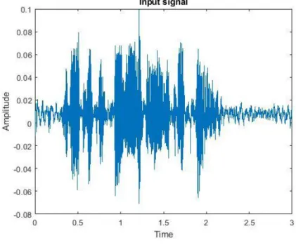
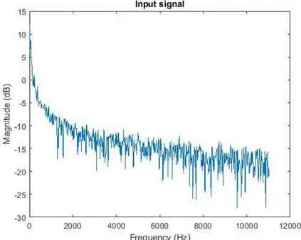
Figures 11 below shows before and after the pre-emphasis filter. A and B shows the speech signal in the time domain, while in C and D the Power Spectrum (PS) is shown in the frequency domain with the sample frequency 44100 Hz.

Figure 11A: Original signal

Figure 11B: Pre-emphasis signal

28

Figure 11C: Original signal (PS)

29 5.2.1.3 Frame Blocking

The next step after pre-emphasis is to split the signal into frame blocks, the frames are usually between 10 to 30 milliseconds. This step is important because in the next steps the use of Fourier transform is used, and it is important to capture the local spectral properties.

To further smooth the transition from one frame to the next frame, a frame overlapping technique is used, the purpose is to approximately center the sequence of the signal. Frame overlapping for MFCC is commonly between 30% to 70%. An overlapping of 50% is used [16][35][36][37], with 20 milliseconds frame size. The frame size is chosen because of the sample frequency which is 44100 Hz, this gives us even samples to overlap by 50%, illustrated in equation 8.

𝑓𝑠× 𝑓𝑟𝑎𝑚𝑒 𝑡𝑖𝑚𝑒

2

= 𝑎𝑚𝑜𝑢𝑛𝑡 𝑜𝑓 𝑜𝑣𝑒𝑟𝑙𝑎𝑝𝑡 𝑠𝑎𝑚𝑝𝑙𝑒𝑠 = 441

5.2.1.4 Hamming Window

In this step a window is used on each frame of the signal. This is needed to remove or reduce any signal discontinuities at the start of the frame and the end of the frame when doing Fourier analysis. For MFCC the most common window used is Hamming window, followed in equation 9 [16][37].

𝑊[𝑛] = 0.54 − 0.46𝑐𝑜𝑠 (2 𝜋𝑛

𝑁−1) (9)

30

Figure 12B: Hamming window on the frame

In figures 12 an illustration is shown on how the hamming window technique works. The plotted frame in A and B is from the same speech signal. One can see in figure 12B that the amplitude at the end and the beginning of the signal is reduced compared to figure 12A.

5.2.1.5 Discrete Fourier Transform

The next step is to take the DFT of each frame with the use of the FFT algorithm seen in equation 10. This is done to extract the spectral information, and to know how much power is contained in the different frequencies [16][17][23][30]. To get the PS then taking the squared amplitude of the DFT is required [5]. The MFCCs are derived from the DFT of the frames along with Mel warping and DCT which will be explained in the next subsections [16][37].

31 5.2.1.6 Mel-Filterbank

The Mel-filterbank is constructed in a way that represent the human ear. Equation 11 below converts Hz to a Mel scale and this gives a linear spacing below 1000 Hz and a logarithmic scaling for the frequencies above 1000 Hz seen in figure 13. To convert from Mel back to Hz can be seen in equation 12 [16][25].

𝑀𝑒𝑙 = 2595𝑙𝑜𝑔10(1 + 𝑓 700−1) (11) 𝑓 = 700(10 𝑀𝑒𝑙 2595− 1) (12)

The next step is to create triangular filters that collect energy in a Mel scale spacing, 32 filter banks are used because it was proven to be the best choice [38], and that the spacing in each filter bank is approximately 120 Mel’s [16]. Figure 13A shows the 32 filterbanks used and figure 13B shows the energies extracted from a single frame.

32

Figure 13B: The energies extracted from a single frame

5.2.1.7 Discrete Cosine Transform

DFT can be split in two parts, the real- and imaginary- part. The real part is the DCT, and the relation between the real axis and the DCT makes it an important part in speech processing [16]. Since the Mel spectrum coefficients are also real numbers then it is possible to convert them to the time domain with DCT [37]. This is the final step to obtain the MFCC features [16][25][30]. From the previous step, one can obtain 32 coefficients that is the same amount of filters used in the Mel filter bank. By obtaining coefficients number 2 to 14, this gives a value of 13 coefficients. Ignoring the first- and the higher- coefficients because it is proven to have less to no relevant information [30].

𝑐_𝑖 = √2 𝑁 ∑ 𝑚𝑗𝑐𝑜𝑠 ( 𝜋𝑖 𝑁(𝑗 − 0.5)) 𝑁 𝑗=1 (13)

33 5.2.2 Normalization and Derivatives

Two feature normalizations will be included to improve the systems performance, CMS and feature warping.

The CMS normalization method is widely used, and is used for robustness against noise, distortion and removes the characteristics of the recording device [12][39]. There are other normalization techniques, but the CMS is more suited for this system because of the use of two microphones and the different effects they bring.

Feature warping reduces EER with 15% compared to using CMS alone [39].

Feature warping consists of mapping the observed cepstral feature distribution to a predefined normal distribution over a sliding window [21].

34

Figure 14B: Normalized distribution of coefficient

The MFCC can be further improved to give better accuracy, this is done by first compute the delta of the MFCC (DMFCCs) this is the first order derivative. It has been proven that the accuracy is even more improved by also using the second order derivative of the MFCC i.e. delta-delta MFCC (DDMFCC) [25][28].

The time derivatives of the MFCCs feature vectors enhance the performance and accuracy. The calculation is for the deltas are followed in equation 14.

𝑑

=

2 ∑𝑁_𝜃=1𝜃2 (14)

In equation 14 the variables 𝑑𝑡are the delta coefficients at the time t, the variable 𝜃is the size of the delta window [14].

35

5.3 The Enrollment Phase

The purpose of the enrollment phase is to create models based on the MFCCs from the feature extraction (MFCC + Delta + Delta Delta) phase. In the enrollment phase a collection of speech is obtained from 650 speakers with 70% male speakers and 30% females speakers to create the imposter model. The GMM and GMM-UBM imposter model has 1024 components and this has been proven to give a better EER compared to 2048, 512, 256 [28]. And the dimensions for this model is the amount of coefficients which are 39 (DDMFCCs). The point of focus for our research question is to create eight true speaker models (eight for GMM and eight for GMM-UBM) for two true speakers, with different amount of training data.

The duration of training data for each model is;

• Model 1 - 0.75 minutes • Model 2 - 1.50 minutes • Model 3 - 3.00 minutes • Model 4 - 6.00 minutes • Model 5 - 12.0 minutes • Model 6 - 24.0 minutes • Model 7 - 48.0 minutes • Model 8 - 60.0 minutes

The results can be seen in chapter 5.4 for each model with the FP and FN along with the EER.

5.4 The Verification Phase

The Verification phase is to verify if the claimed speaker is an imposter or a true speaker. There are sixteen true speaker models for two speakers, a new collection of data is used to verify the models created and to obtain the results from it. The true speakers collects 150 new utterances with 3 seconds duration per utterance, and then ten imposter speakers that are not registered in the imposter model collects 15 utterances with 3 seconds duration per utterance. The scores can be seen in the tables in subsection 5.4.

36

5.5 Results

The results are presented in the tables below, with sixteen models for each speaker, and each model has a training data from 45 seconds up to 1 hour. The FN and FP in the table are based on 12 speakers and a variation of the threshold is also illustrated.

An explanation of the columns in table 2, 3, 4, 5.

• Model - The duration of the amount of training data for each model.

• Min & Max - The minimum and maximum score achieved from the speakers

• True speaker - The score of the true speaker with minimum and maximum score obtained from 150 trials.

• Imposter Speakers - The score of the imposter speakers with minimum and maximum score obtained from 150 trials.

• FP - The amount of FP if the threshold is set at the minimum value of the true speaker score (no FN)

• FN - How many times the system does not recognize the true speaker from a set of 150 trials with a threshold that is set at the maximum imposter speaker score (no FP).

• EER - Is the Equal Error Rate where the tradeoff is equal between FPR and FNR E.g. in table 2, the column “Model One" shows the duration of the training data with 45 seconds, the “FP and FN” columns show that the FP is 18 and FN is 16, and the EER is set to 4,6667

37 5.5.1 The GMM-UBM Method

This subsection presents the results obtained with the GMM-UBM models.

Speaker One GMM-UBM Model Min & Max

Score

True Speaker Imposter Speakers

FP (of 150)2 _{FN (of 150)}3 _{EER (%)}

One (45 sec) Min Score 0,00870769 -0,00402882 18 16 4,6667 Max Score 0,028357148 0,013626177

Two (1.5 min) Min Score 0,018041779 -0,00617504 16 11 4,0000 Max Score 0,057024557 0,025695847

Three (3 min) Min Score 0,034247064 -0,011665563 19 12 3,3333 Max Score 0,110756034 0, 048805133

Four (6 min) Min Score 0,062659219 -0,022923001 22 13 3,333 Max Score 0,201937702 0,094237107

Five (12 min) Min Score 0,117817102 -0,033097339 15 9 1.3333 Max Score 0,375977933 0,174932044

Six (24 min) Min Score 0,197142321 -0,05674105 7 11 1,3333 Max Score 0,62512666 0,276985393

Seven (48 min) Min Score 0,306788539 -0,081925837 3 3 1,3333 Max Score 0,867689006 0,365730796

Eighth (60 min) Min Score 0,336153946 -0,09077135 3 3 1,3333 Max Score 0,987862643 0,395860276

Table 2: Results for speaker one based on eight models with different amount training data with GMM-UMB modeling.

2 _{If the threshold is set at the minimum value for the true speaker (no false negatives)} 3 _{If the threshold is set above the maximum false speakers (no False Positives)}

38

Speaker Two GMM-UBM Model Min & Max

Score

True speaker Imposter Speaker FP (of 150)4 _{FN (of 150)}5 _{EER (%)}

One (45 sec) Min Score 0,006600232 -0,000970263 74 45 12,6667 Max Score 0,031390045 0,014656359

Two (1.5 min) Min Score 0,008591385 -0,003094435 113 19 4,6667 Max Score 0,06315318 0,027028485

Three (3 min) Min Score 0,016512423 -0,005580669 86 28 8,0000 Max Score 0,120073816 0,046244904

Four (6 min) Min Score 0,019319328 -0,009219546 108 48 13,3333 Max Score 0,235497945 0,09150491

Five (12 min) Min Score 0,026853545 -0,019185077 129 55 16,0000 Max Score 0,45612731 0,187558776

Six (24 min) Min Score 0,124529395 -0,022079607 69 27 3,3333 Max Score 0,549137165 0,289817779

Seven (48 min) Min Score 0,296393203 -0,049911876 21 4 0,6667 Max Score 0,780212116 0,381950347

Eighth (60 min) Min Score 0,418886003 -0,064965486 3 1 0,6667 Max Score 0,967036527 0,426439902

Table 3: Results for speaker two based on eight models with different amount training data with GMM-UMB modelling.

4 _{If the threshold is set at the minimum value for the true speaker (no false negatives)} 5 _{If the threshold is set above the maximum false speakers (no False Positives)}

39

The score distribution comparison between the true speaker and imposter speakers trials from the experiment, are shown in the figures 15 below for two models (model one and model eight). These figures show the score collisions between the imposters and the true speakers and the amount of trials colliding. This gives an understanding for more data gives less collision e.g. in model eight compared to model one.

Figure 15A: Shows the score distribution for model one between the true speaker and imposter speaker (speaker one).

Figure 15B: Shows the score distribution for model eight between the true speaker and imposter speaker (speaker one).

40

Figure 15C: Shows the score distribution for model one between the true speaker and imposter speaker (speaker two).

Figure 15D: Shows the score distribution for model eight between the true speaker and imposter speaker (speaker two).

The DET curves for the results are illustrated in figures 16 for the two true speakers (model one and model eight), as mentioned the threshold is varied as seen in table 2 and

41

3 for best FP or FN and this is dependent of the system application if there is a need for high security (e.g. door access control or turn on a lightbulb at home) or not.

Figure 16A: Shows the DET curve for model one (speaker one).

42

Figure 16C: Shows the DET curve for model one (speaker two).