Experimental and theoretical lifetimes and transition probabilities for spectral lines in Nb II

https://doi.org/10.1051/0004-6361/201935614 c ESO 2019

Astronomy

&

Astrophysics

Experimental and theoretical lifetimes and transition probabilities

for spectral lines in Nb ii

H. Nilsson

, L. Engström

, H. Lundberg

, H. Hartman

, P. Palmeri

, and P. Quinet

e-mail: hampus.nilsson@astro.lu.se

2 _{Department of Physics, Lund University, Box 118, 22100 Lund, Sweden}

3 _{Materials Science and Applied Mathematics, Malmö University, 20506 Malmö, Sweden} 4 _{Physique Atomique et Astrophysique, Université de Mons, 7000 Mons, Belgium} 5 _{IPNAS, Université de Liège, 4000 Liège, Belgium}

Received 4 April 2019/ Accepted 30 May 2019

ABSTRACT

Aims. We have measured and calculated lifetimes of high lying levels in Nb ii, and derived absolute transition probabilities by com-bining the lifetimes with experimental branching fractions.

Methods. The lifetimes were measured using time-resolved laser-induced fluorescence in a two-photon and two-step excitation scheme. The branching fractions were measured in intensity calibrated spectra from a hollow cathode discharge, recorded with a Fourier transform spectrometer. The calculations were performed with the relativistic Hartree–Fock method including core polarization.

Results. We report experimental lifetimes of 13 levels in the 4d3₍4_{F)5d and 4d}3₍4_{F)6s subconfigurations, at an energy around}

70 000 cm−1_{. By combining the lifetimes with experimental branching fractions absolute transition probabilities of 59 lines are}

derived. The experimental results are compared with calculated values.

Key words. atomic data – methods: laboratory: atomic – techniques: spectroscopic

1. Introduction

Niobium was discovered in 1801 by the British chemist Charles Hatchett. The element was discovered in the mineral columbite, and Hatchett gave the element the name columbium (Cb). In 1844 Heinrich Rose reported two new elements, niobium, and penopium. However, Jean-Charles de Marignac showed that the elements columbium, niobium and penopium were in fact all the same. The name columbium was in use until 1949 when nio-bium was adopted as the official name of element number 41. The Swedish chemist Christian Blomstrand is believed to be the first one to isolate niobium. The fascinating history of niobium, columbium, pelopium, and tantalum and Charles Hatchett can be found inGriffith & Morris(2003).

Niobium is a key element to understand and probe the slow-neutron-capture process (the s-process). Niobium is monoiso-topic (93Nb) and believed to be mainly produced by β decay of 93_{Zr, with a half-life of τ}

1/2 = 1.53 × 106yr. The proba-bility of 93Zr capturing a neutron and producing 94Zr is larger than that of93_{Zr decaying to}93_{Nb as long as the s-process is} ongoing. Hence the niobium abundance can give the time since the s-process ended (Smith & Lambert 1984). Furthermore, by comparing the ratios 93_Zr/93_{Nb and} 99_Tc/99_{Ru it is possible} to determine the s-process temperature and the time since the s-process started (Neyskens et al. 2015).

In 1935 Meggers & Schribner (1935) published a paper reporting the term analysis of the first two spectra, Cb i and Cb ii (arc and spark) of columbium, including 2000 lines combining 60 levels in Cb ii. The analysis was extended by Humpreys & Meggers(1945) who reported 183 levels in Cb ii. InIglesias(1954) a study of the vacuum ultraviolet spectrum was

reported, identifying 20 new energy levels and 330 spectral lines as belonging to Nb ii (this is the first term analysis paper using the name niobium instead of columbium). The most recent term analysis of Nb ii is reported byRyabtsev et al.(2000), based on spectra recorded with Fourier transform spectroscopy. A total of 353 energy levels in Nb ii are presently known from the work reported in these papers.

Experimental transition probabilities in Nb ii have been reported by Hannaford et al. (1985), by combining radiative lifetimes of 27 levels with branching fractions (BFs) derived from the work ofCorliss & Bozman(1962).Nilsson & Ivarsson (2008) reported transition probabilities for 145 lines combining BFs measured in Fourier transform spectra with the lifetimes reported by Hannaford et al. (1985). In Nilsson et al. (2010) additional transition probabilities were reported for lines from the 4d3 _{5p configuration derived from lifetimes combined with} BFs, along with new theoretical calculations.

Niobium has one stable isotope, 93_{Nb, which has an odd} number of nucleons. Due to the nuclear spin I= 9/2 and a large magnetic moment, µ = 6.1705 µN (Mills et al. 1988), many of the spectral lines show large hyperfine structure (hfs). Experi-mental measurements of hfs has been reported byYoung et al. (1995) and Nilsson & Ivarsson (2008). However, none of the lines reported in the present work are noticeably affected by hfs. In this work we report experimental transition probabilities for 59 lines originating from 13 levels in the 4d3₍4_{F)5d and} 4d3₍4_{F)6s subconfigurations, derived by combining branching} fractions and radiative lifetimes. These new data are compared with semi-empirical calculations performed using a relativistic Hartree-Fock model including core-polarization effects.

2. Laboratory measurements

2.1. Lifetimes

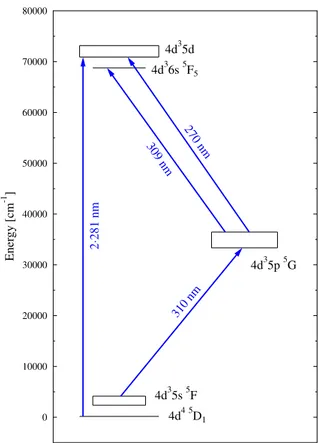
The spectrum and term system of Nb ii have been thoroughly investigated byRyabtsev et al.(2000). This work was essential not only to find the investigated levels but also to check for pos-sible blending, as discussed below. The ground term in Nb ii is the even 4d4 5_{D, with levels between 0 and 1200 cm}−1_{, and} the second lowest even term is 4d3₍4_F)5s5_{F between 2300 and} 4150 cm−1_{. To reach the investigated high lying even 5d and} 6s levels, between 68 000 and 73 200 cm−1, we employed either two-photon excitations using a single laser or a two-step pro-cedure where the first laser excited intermediate odd levels in the 4d3₍4_F)5p5_{G term from which the second laser reached the} 5d and 6s levels. Figure1illustrates the levels and wavelengths involved, and Table 1 gives the detailed excitation scheme for each level.

The experimental setup for two-photon and two-step mea-surements at the high-power laser facility at the University of Lund is described in detail in Engström et al. (2014) and Lundberg et al.(2016) and only the most important details will be given here. The setup includes three Nd:YAG lasers operating at 10 Hz. The frequency-doubled output of one of them (Contin-uum Surelite) is focused on a rotating niobium target in a vac(Contin-uum chamber with a pressure of about 10−4mbar to produce the nio-bium ions through laser ablation. Interactions with the electrons in the created plasma also excite the even 4d4and 4d35s config-urations, which contain the starting levels in our experiments.

For the two-step measurements, the second Nd:YAG (Con-tinuum NY-82) laser pumps a dye laser (Con(Con-tinuum Nd-60) which, after frequency-doubling, produces a 10 ns long pulse for the first excitation to the odd 4d3₍4_F)5p5_{G levels. A similar} laser combination is used for the second step, but here the output of the Nd:YAG laser is temporally compressed using Brillouin scattering in water before pumping the dye laser. The frequency-doubled light from the dye laser is then passed through a tube with hydrogen gas where a Stokes shift of 4153 cm−1_{could be} added. The final length, full width at half maximum (FWHM), of the second step pulse was about 1 ns.

Both laser pulses intersected the niobium plasma from the same direction at right angles to the ablation laser a few millime-ter above the niobium target. The timing between the two excita-tions is very important and adjusted so that the second step laser coincided in time with the maximum fluorescence from the inter-mediate level. Because of the difference in pulse length between the two lasers this ensures that the intermediate level popula-tion is constant during the second excitapopula-tion. For the two-photon measurements only the short pulses from the second laser were used.

The fluorescence from the excited levels was observed with a small f/8 monochromator, with its 120 µm wide entrance slit parallel to the excitation lasers, in a direction perpendicular to all three laser beams. The observed line width (FWHM) was 0.5 nm in the second spectral order. The time varying signal was reg-istered with a microchannel-plate photomultiplier (Hamamatsu R3809U) with a rise time of 0.15 ns, and digitized by a Tektronix DPO 7254 oscilloscope in time intervals of 50 ps. A second channel on the oscilloscope sampled simultaneously the tempo-ral shape of the short-pulsed (1 ns) laser obtained from a fast photodiode. Each decay curve and pulse shape was averaged over 1000 laser shots. Between 10 and 20 decay curves were recorded for each level. The lifetimes were determined by fitting a single exponential decay, convoluted by the measured shape of the second step laser, and a constant background using the

0 10000 20000 30000 40000 50000 60000 70000 80000 Ener gy [cm -1 ] 4d4 5D₁ 4d35s5F 4d35p5G 4d36s5F5 4d35d 2 281 nm 310 nm 309 nm 270 nm

Fig. 1.Schematic term system for Nb ii showing the investigated

lev-els and the typical wavelengths used for the two-photon and two-step excitations.

software DECFIT (Palmeri et al. 2008). In the two-photon case, the square of the measured excitation pulse was used.

In the two-step measurements some corrections of the recorded decay curves were necessary before the fitting proce-dure. In the case of 5d5_H

6,7the only sufficiently intense decay channels were the same as those used for the second step excita-tion. This resulted in a contamination of the decay by scattered laser light. However, this effect was taken care of by recording a decay curve for the second laser either at a wavelength slightly off resonance or with the first step laser blocked. This mea-surement was then subtracted from the observed primary decay before the lifetime extraction. Figure2 illustrates this problem for 5d5_H

6, which was the worst case observed. Another prob-lem was encountered in most cases because the very intense and long-lived fluorescence from the intermediate level could pro-duce a small but noticeable contribution in the measured decay channel even at substantial wavelength differences. Similar to the previous example, this could be handled by recording and subtracting the signal from the intermediate level with the sec-ond step laser blocked. Finally, for both photon and two-step measurements, uncorrectable blending problem may arise from cascades, that is intermediate levels being populated from the level under investigation that in turn decay with wavelengths close to the investigated decay channel. This problem precluded for example the measurement of the 5d5_G

4level. To search for such effects, detailed spectroscopic studies, such as the one by Ryabtsev et al.(2000), are essential.

The excitation schemes employed and the final experimental lifetimes are presented in Table1. The quoted uncertainties are based on the variations between the repeated measurements that include tests to ascertain the absence of systematic effect. Exam-ples of the latter effects are the variations in the lifetimes with

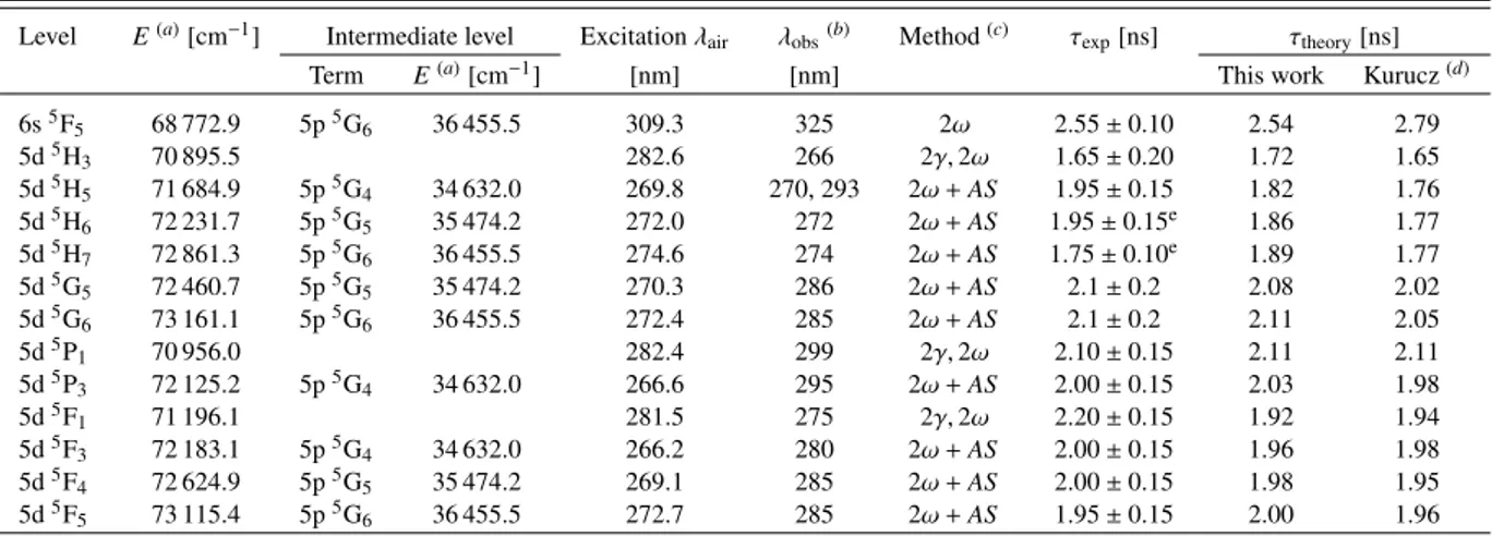
Table 1. Experimental details and the measured and calculated lifetimes of the levels in Nb ii.

Level E(a)_[cm−1_{] Intermediate level Excitation λ}

air λobs(b) Method(c) τexp[ns] τtheory[ns]

Term E(a)_[cm−1_{] [nm] [nm] This work Kurucz}(d)

6s5_F 5 68 772.9 5p5G6 36 455.5 309.3 325 2ω 2.55 ± 0.10 2.54 2.79 5d5_H 3 70 895.5 282.6 266 2γ, 2ω 1.65 ± 0.20 1.72 1.65 5d5_H 5 71 684.9 5p5G4 34 632.0 269.8 270, 293 2ω+ AS 1.95 ± 0.15 1.82 1.76 5d5_H 6 72 231.7 5p5G5 35 474.2 272.0 272 2ω+ AS 1.95 ± 0.15e 1.86 1.77 5d5_H 7 72 861.3 5p5G6 36 455.5 274.6 274 2ω+ AS 1.75 ± 0.10e 1.89 1.77 5d5_G 5 72 460.7 5p5G5 35 474.2 270.3 286 2ω+ AS 2.1 ± 0.2 2.08 2.02 5d5_G 6 73 161.1 5p5G6 36 455.5 272.4 285 2ω+ AS 2.1 ± 0.2 2.11 2.05 5d5_P 1 70 956.0 282.4 299 2γ, 2ω 2.10 ± 0.15 2.11 2.11 5d5_P 3 72 125.2 5p5G4 34 632.0 266.6 295 2ω+ AS 2.00 ± 0.15 2.03 1.98 5d5_F 1 71 196.1 281.5 275 2γ, 2ω 2.20 ± 0.15 1.92 1.94 5d5_F 3 72 183.1 5p5G4 34 632.0 266.2 280 2ω+ AS 2.00 ± 0.15 1.96 1.98 5d5F4 72 624.9 5p5G5 35 474.2 269.1 285 2ω+ AS 2.00 ± 0.15 1.98 1.95 5d5F5 73 115.4 5p5G6 36 455.5 272.7 285 2ω+ AS 1.95 ± 0.15 2.00 1.96

Notes. (a)_{Ryabtsev et al. (2000).}(b)_{All fluorescence measurements were performed in the second spectral order.}(c)_{2ω means the second}

har-monic of the dye laser, AS means one added Stokes shift (4153 cm−1_{) and 2γ means two-photon excitation.}(d)_{Semi-empirical}

superposition-of-configurations calculation byKurucz(2017).(e)_{Corrected for scattered light from the second step laser.}

0 2300 4600 0 5 10 15 20 25 Time [ns] In te n s ity [ a rb . u n its ]

Fig. 2. Measured decay curve for the 4d3_5d 5_H

6 level (+) and the

recorded second step laser pulse (−). The dashed curve is a recording of the scattered light from the second step laser at a slightly detuned wave-length. This measurement is then subtracted from the real decay before the lifetime determination. The actual measurement extends to 40 ns.

and without the small correction for the background contribution from the intermediate levels, discussed above, and the search for saturation effects by inserting a varying number of neutral den-sity filters in the second step laser beam. Furthermore, possible flight effects (Sikström et al. 2002) were investigated by vary-ing the delay between the ablation and excitation lasers, which results in ions with different velocities arriving in the interaction zone at a fixed distance from the target.

2.2. Branching fractions and transition probabilities

The branching fraction (BF) of a line is defined as the transition probability of the line divided by the sum of transition probabili-ties for all lines from the same upper level, that is the inverse of the lifetime (τ). Hence, if one can measure the intensity of all transitions from one upper level, transition probabilities can be derived by combining the BFs with radiative lifetimes according to BFul = Iul/ P

k=1

Iukand Aul = BFul/τu. To convert the transi-tion probabilities to oscillator strengths ( f ), the following relatransi-tion can be used: g_lflu= (λ/258.27)2guAul, where gl(u)is the statistical weight of the lower (upper) level, with λ in nm and A in (ns)−1_.

However, some lines can be too weak to be measured, but the total BF of all missing lines can be estimated from theoretical calculations. This correction is called the residual and is given in TableA.1for each level.

The niobium spectra where produced in a hollow cathode discharge with a mixture of neon and argon as carrier gas (at a current of 0.6 A and a pressure of 1 Torr), and recorded using the Lund Observatory Chelsea Instruments FT500 UV Fourier transform spectrometer, with a resolution of 0.035 cm−1. Two spectra were used. The first, covering the wavenumber region 20 000–40 000 cm−1(250–500 nm), was recorded with a Hama-matsu R955 optical photomultiplier tube. The second spectrum (28 000–56 000 cm−1, 180–360 nm) was recorded with a Hama-matsu R166 solar blind photomultiplier tube. The spectra were intensity calibrated using branching ratios in argon (from 20 000 to 35 000 cm−1, 290–500 nm) reported byWhaling et al.(1993), and a deuterium lamp calibrated by Physicalisch-Technische Bundesanstalt, Berlin, Germany (30 000–50 000 cm−1, 200– 330 nm). The calibration procedure is further discussed in Sikström et al.(2002).

The uncertainties in the BFs include the uncertainty in the intensity measurements and the uncertainty in the intensity cali-bration, not only in the line itself, but also in the other lines from the same upper level, as they influence the derived value of the BF. The method to estimate uncertainties is described in detail in Sikström et al.(2002). The derived BFs and log(g f ) values are given in TableA.1. The BFs are compared with theoretical val-ues from this work and valval-ues fromKurucz(2017). In addition, we present the uncertainties both in the BFs and in the g f -values. The uncertainty in the g f -values includes the uncertainty both in the BF and the lifetime.

In most cases the lines were easy to identify thanks to the thorough analysis byRyabtsev et al.(2000). However, we found a few lines that were blended or misidentified. The transition 4d3₍4_F)5p5_F

3– 4d3(4F)5d5P3at 34 748.346 cm−1(287.7 nm) is blended with a weak hfs pattern, as seen in Fig.3. The intensity of the line is corrected by measuring the intensity of the adja-cent hfs components to estimate the blending contribution. The correction changed the BF of this line from 0.40 to 0.35.

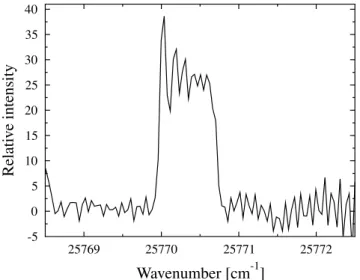
The line at 25 770.230 cm−1 (387.9 nm) is identified by Ryabtsev et al.(2000) as 4d3₍2_H)5p3_H

4– 4d3(4F)5d5F5. How-ever, as suggested byNilsson et al.(2010), this is probably the

0 10 20 30 40 50 60 70

Relati

v

e

intensity

Wavenumber [cm

]

3– 4d3(4F)5d5P3transition, marked with the arrow.

The line is blended with the wide hfs pattern of an unidentified line. The blending intensity is estimated with the adjacent hfs components (see text). -5 0 5 10 15 20 25 30 35 40

Relati

v

e

intensity

Wavenumber [cm

]

4 – 4d3(4F)5p z3F4 transition. The line is wrongly

assigned as 4d3₍2_H)5p3_H

4– 4d3(4F)5d5F5transition byRyabtsev et al.

(2000) (see text).

4d4 a1G4 – 4d3(4F)5p z3F4 transition instead, which has a Ritz wavenumber of 25 770.263 cm−1_{. Furthermore, this} identifica-tion is strengthened by analysing the hfs pattern (as can be seen in Fig. 4) of the line, which is consistent with the split-tings in the two levels, 4d4a1G4and 4d3(4F)5p z3F4, reported by

Nilsson & Ivarsson(2008).

The line at 32 554.352 cm−1 _{(307.1 nm) is identified by}

Ryabtsev et al.(2000) as 4d3(4F)5p3F4 – 4d3(4F)5d5F5. How-ever, this coincides with the 4d4_a1_G

4– 4d3(2H)5p3H4transition (with the Ritz wavenumber 32 554.359 cm−1) which, accord-ing to our calculations, has a transition probability that is orders of magnitude larger. We therefore conclude that the two lines 25 770.230 cm−1_{and 32 554.352 cm}−1_{are misidentified by}

Ryabtsev et al.(2000), and we have excluded them in the analy-sis of the level 4d3₍4_F)5d5_F

5at 73 115.352 cm−1.

In most cases the residual is small (between 0.4 and 4.1%). However, for the 4d3(4F)5d 5P1 and 4d3(4F)5d5F1 transitions, the residuals are larger 14.4 and 31.3%, respectively). This is

-0.5 -0.4 -0.3 -0.2 -0.1 0.0 0.1 0.2 0.3 0.4 0.5

BF

-BF

BFexp

Fig. 5. Comparison between our experimental BFs and theoretical

values.

because that the population is proportional to the statistical weight, g= 2J + 1, so lines from levels with J = 1 have a lower signal to noise ratio, and some of the lines therefore become too weak to be measured. However, the lines that are measured are in good agreement with the theoretical values, if scaled with the residual. The uncertainties for these two levels will perhaps be overestimated as the residual is given an uncertainty of 50%.

For the levels 4d3₍4_F)5d5_P

3and 4d3(4F)5d5F3, both J= 3, a poor agreement between experiment and theory is seen. We find no experimental reason for this, but it can be noted that the two different calculations are not in agreement for these two levels. Because of the poor agreement between experiment and theory we have not included residuals for these levels. This may over-estimate the BFs from these levels slightly.

3. Semi-empirical calculations

The experimental radiative parameters measured in the present work are compared with theoretical results obtained using the pseudo-relativistic Hartree–Fock (HFR) method of Cowan (1981) modified to take core-polarization effects (HFR+CPOL) into account, as described fore example byQuinet et al.(1999, 2002). The calculations are based on the same physical model as the one assumed to be best (referred to as HFR(B)) in our pre-vious work on Nb II (Nilsson et al. 2010). As a reminder, in this model the intravalence interactions were considered by explicitly including the following multi-configuration expansions: 4d4 + 4d3_{5s+ 4d}3_{6s+ 4d}3_{5d+ 4d}2_5s2_{+ 4d}2_5p2_{+ 4d}2_{5s6s+ 4d}2_5s5d + 4d2_{4f5p+ 4d}2_{5p5f+ 4d}2_6s2_{+ 4d}2_5d2_{+ 4d}2_{5d6s+ 4d}2_5p6p for the even parity, and 4d3_{5p + 4d}3_{6p + 4d}3_{4f + 4d}3_{5f +} 4d2_{5s5p+ 4d}2_{5s6p+ 4d}2_{4f5s+ 4d}2_{4f5d+ 4d}2_{5s5f+ 4d}2_5p6s+ 4d25p5d+ 4d26s6p for the odd parity. Using the well-established least-squares approach that minimizes the differences between the calculated and the available experimental energy levels pub-lished by Ryabtsev et al. (2000), some radial parameters were optimized according to the methodology described in detail by Nilsson et al. (2010). The core-polarization effects were first estimated using the dipole polarizability corresponding to the ionic Nb IV core given inFraga et al.(1976), αd= 5.80a3₀, while the cut-off radius (rc) was chosen to be the mean value hri of the outermost 4d core orbital, rc = 1.85a0. Using these two param-eters, we found that our calculated lifetimes were systematically

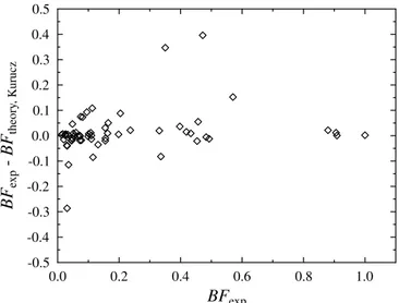
-0.5 -0.4 -0.3 -0.2 -0.1 0.0 0.1 0.2 0.3 0.4 0.5

BF

-BF

BFexp

Fig. 6.Comparison between our experimental BFs and theoretical

val-ues fromKurucz(2017).

a few percent longer than those measured in the present work for 4d36s and 4d35d levels. Therefore, we adjusted semi-empirically the dipole radial integrals of the 4d3_{5p – 4d}3_{6s and 4d}3_{5p –} 4d35d transitions to fit the calculations to the experimental life-times. This gave rise to the values h5p|r|6si = −2.64 a.u. and h5p|r|5di= −5.74 a.u., that being respectively 6% and 9% larger than the values obtained using the HFR(B) model considered in our previous paper (Nilsson et al. 2010).

The calculated lifetimes are compared with the experimental measurements in Table1. We can clearly note that our calculated values fall within the experimental uncertainties, the average ratio τCalc/τExpbeing equal to 0.99 ± 0.05 where the uncertainty represents the standard deviation from the mean. This agreement is similar to (but slightly better than) the one obtained when comparing the theoretical data from Kurucz (2017) with the experimental lifetimes (τKurucz/τExp= 0.98±0.06). In TableA.1, the BFs calculated in the present work are compared with the experimental values and the theoretical results deduced from the work of Kurucz (2017). These comparisons are illustrated in Figs.5and6. It can be seen that our computed values are gen-erally in better agreement with the experimental values (stan-dard deviation ∆σ = 0.067) than those from Kurucz (2017) (∆σ = 0.089). However, for two upper even levels, those located at 72 125.247 and 72 183.090 cm−1, rather large discrepancies (up to two orders of magnitude) are observed when comparing the theoretical BFs with the measurements. This is mainly due to the strong mixings characterizing not only the upper but also the lower levels involved in the transitions. More precisely, accord-ing to our calculations, the main LS components of the levels at 72 125.247 and 72 183.090 cm−1 _{are 81% 5d}5_P

3 + 13% 5d

3_D

3+ 2% 5d5F3and 60% 5d5F3+ 33% 5d5G3+ 2% 5d3D3, respectively. Both of them have, for example, one transition to the 5p 5F3 lower level (E = 37 376.901 cm−1), for which the theoretical and experimental BFs disagree. In fact, for this latter level, our calculations give a strongly mixed eigenvector, 53% 5p 5F3 + 25% 5p 3D3 + 7% 5p 5D3, giving rise to transition

decay rates for the lines at 2876.991 and 2872.209 Å, which are very sensitive to small changes in the eigenvector compositions, both for the upper 5d and lower 5p levels. Moreover, both lev-els at 72 125.247 and 72 183.090 cm−1are depopulated by quite a large number of very weak lines (contributing to the residuals given in TableA.1), which are affected by strong cancellation effects in our calculations (see Cowan 1981). This makes the determination of BFs less reliable for these two levels.

4. Summary

We report experimental and theoretical radiative lifetimes for high lying even 4d3 5d and 6s levels, between 68 000 and 73 200 cm−1 _{in Nb ii. In addition, we have measured BFs for} 59 lines depopulating the levels. Combing the lifetimes with the BFs has generated absolute transition probabilities for the lines. The experimental values are compared with theoretical data, both new data reported in this work and values from the literature (Kurucz 2017).

Acknowledgements. This work was supported by the Swedish Research Coun-cil through the Linnaeus grant to the Lund Laser Centre and the Knut and Alice Wallenberg Foundation. This work was financially supported by the Integrated Initiative of Infrastructure Project LASERLAB-EUROPE, contract LLC002130. H.H acknowledges the Swedish Research Council Grant 2016-04185. P.P. and P.Q. are respectively Research Associate and Research Director of the Belgian Fund for Scientific Research F.R.S.-FNRS. Financial support from this organi-zation is sincerely acknowledged.

References

Corliss, C. H., & Bozman, W. R. 1962,Natl. Bur. Stand. (US) Monogr., 53

(Washington, D.C.: US Department of Commerce)

Cowan, R. D. 1981,The Theory of Atomic Structure and Spectra(Berkeley: Univ. California Press)

Engström, L., Lundberg, H., Nilsson, H., Hartman, H., & Bäckström, E. 2014,

A&A, 570, A34

Fraga, S., Karwowski, J., & Saxena, K. M. S. 1976,Handbook of Atomic Data

(Amsterdam: Elsevier)

Griffith, W. P., & Morris, P. J. T. 2003,Notes Rec. R. Soc. Lond., 57, 299

Hannaford, P., Lowe, R. M., Biemont, E., & Grevesse, N. 1985,A&A, 143, 447

Humpreys, C. J., & Meggers, W. F. 1945,Res. Nat. Bur. Stand. (U.S.), 43, 481

Iglesias, L. 1954,An. Real Soc. Esp. Fys. Quim. (Madrid), 50, 135

Kurucz, R. L. 2017, Available athttp://kurucz.harvard.edu/atoms.html

[accessed June 18]

Lundberg, H., Hartman, H., Engström, L., et al. 2016,MNRAS, 460, 356

Meggers, W. F., & Schribner, B. F. 1935,J. Res. Natl. Bur. Stand. (U.S.), 14, 629

Mills, I., Cvitas, T., Homann, K., Kallay, N., & Kuchitsu, K. 1988,Quantities, Units and Symbols in Physical Chemistry(Oxford, UK: Blackwell Scientific Publications) [Copyright 1988 IUPAC]

Nilsson, H., & Ivarsson, S. 2008,A&A, 492, 609

Nilsson, H., Hartman, H., Engström, L., et al. 2010,A&A, 511, A16

Neyskens, P., Van Eck, S., Jorissen, A., et al. 2015,Nature, 517, 174

Palmeri, P., Quinet, P., Fivet, V., et al. 2008,Phys. Scr., 78, 015304

Quinet, P., Palmeri, P., Biémont, E., et al. 1999,MNRAS, 307, 934

Quinet, P., Palmeri, P., Biémont, E., et al. 2002,J. Alloys Comp., 344, 255

Ryabtsev, A. N., Churilov, S. S., & Litzén, U. 2000,Phys. Scr., 62, 368

Sikström, C. M., Nilsson, H., Litzén, U., Blom, A., & Lundberg, H. 2002,J. Quant. Spectrosc. Radiat. Transfer, 74, 355

Smith, V. V., & Lambert, D. L. 1984,Publ. Astron. Soc. Pac., 96, 226

Whaling, W., Carle, M. T., & Pitt, M. L. 1993,J. Quant. Spec. Radiat. Transf., 50, 7

Young, L., Hasegawa, S., Kurtz, C., Datta, D., & Beck, D. R. 1995,Phys. Rev. A, 51, 3534

Appendix A: Additional table

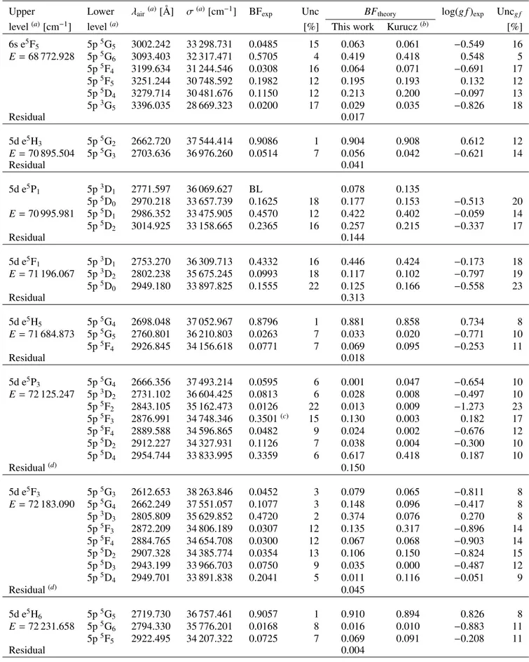
Table A.1. Experimental and theoretical branching fractions for transitions in Nb ii.

Upper Lower λair(a)[Å] σ(a)[cm−1] BFexp Unc BFtheory log(g f )exp Uncg f

level(a)[cm−1] level(a) [%] This work Kurucz(b) [%]

6s e5F5 5p5G5 3002.242 33 298.731 0.0485 15 0.063 0.061 −0.549 16 E= 68 772.928 5p5_G 6 3093.403 32 317.471 0.5705 4 0.419 0.418 0.548 5 5p5_F 4 3199.634 31 244.546 0.0308 16 0.064 0.071 −0.691 17 5p5_F 5 3251.244 30 748.592 0.1982 12 0.195 0.193 0.132 12 5p5_D 4 3279.714 30 481.676 0.1150 12 0.213 0.200 −0.097 13 5p3G5 3396.035 28 669.323 0.0200 17 0.029 0.035 −0.826 18 Residual 0.017 5d e5H3 5p5G2 2662.720 37 544.414 0.9086 1 0.904 0.908 0.612 12 E= 70 895.504 5p5_G 3 2703.636 36 976.260 0.0514 7 0.056 0.042 −0.621 14 Residual 0.041 5d e5_P 1 5p3D1 2771.597 36 069.627 BL 0.078 0.135 5p5D0 2970.218 33 657.739 0.1625 18 0.177 0.153 −0.513 20 E= 70 995.981 5p5_D 1 2986.352 33 475.905 0.4570 12 0.422 0.402 −0.059 14 5p5D2 3014.925 33 158.665 0.2365 16 0.257 0.215 −0.337 17 Residual 0.144 5d e5F1 5p3D1 2753.270 36 309.713 0.4332 16 0.446 0.424 −0.173 18 E= 71 196.067 5p3_D 2 2802.238 35 675.245 0.0993 18 0.117 0.102 −0.797 19 5p5D0 2949.180 33 897.825 0.1555 22 0.125 0.166 −0.558 23 Residual 0.313 5d e5H5 5p5G4 2698.048 37 052.967 0.8796 1 0.881 0.858 0.734 8 E= 71 684.873 5p5_G 5 2760.801 36 210.803 0.0263 7 0.033 0.020 −0.771 10 5p5F4 2926.845 34 156.618 0.0771 7 0.069 0.095 −0.253 11 Residual 0.018 5d e5P3 5p5G4 2666.356 37 493.214 0.0595 6 0.001 0.047 −0.654 10 E= 72 125.247 5p3D2 2731.102 36 604.425 0.0813 6 0.028 0.008 −0.497 10 5p5_F 2 2843.105 35 162.473 0.0126 22 0.013 0.009 −1.273 23 5p5F3 2876.991 34 748.346 0.3501(c) 15 0.130 0.003 0.182 17 5p5_F 4 2889.588 34 596.865 0.0482 9 0.024 0.002 −0.676 12 5p5D2 2912.227 34 327.931 0.1126 7 0.038 0.004 −0.300 10 5p5_D 4 2954.744 33 833.995 0.3359 6 0.617 0.418 0.187 10 Residual(d) 0.150 5d e5_F 3 5p5G3 2612.653 38 263.846 0.0452 3 0.079 0.065 −0.811 8 E= 72 183.090 5p5G4 2662.249 37 551.057 0.1077 3 0.148 0.096 −0.417 8 5p3_D 3 2805.809 35 629.852 0.4720 2 0.374 0.076 0.270 8 5p5F3 2872.209 34 806.189 0.0307 12 0.135 0.317 −0.896 14 5p5_F 4 2884.765 34 654.708 0.0300 12 0.067 0.068 −0.903 14 5p5D2 2907.328 34 385.774 0.0354 13 0.106 0.150 −0.824 15 5p5_D 3 2943.199 33 966.703 0.0750 9 0.035 0.000 −0.487 12 5p5D4 2949.701 33 891.838 0.2041 5 0.011 0.116 −0.051 9 Residual(d) _0.045 5d e5H6 5p5G5 2719.730 36 757.461 0.9057 1 0.910 0.894 0.826 8 E= 72 231.658 5p5_G 6 2794.330 35 776.201 0.0168 8 0.016 0.010 −0.883 11 5p5F5 2922.495 34 207.322 0.0725 7 0.069 0.091 −0.208 11 Residual 0.004

Notes.(c)_{Corrected for blend (see text).}(d)_{Residual not included in these levels (see text).}

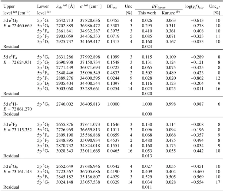
Table A.2. continued.

Upper Lower λair(a)[Å] σ(a)[cm−1] BFexp Unc BFtheory log(g f )exp Uncg f

level(a)_[cm−1_{] level}(a) _{[%] This work Kurucz}(b) _[%]

5d e5_G 5 5p5G4 2642.713 37 828.636 0.0455 4 0.026 0.063 −0.613 10 E= 72 460.669 5p5G5 2702.889 36 986.472 0.3307 3 0.295 0.311 0.278 10 5p5_F 4 2861.841 34 932.287 0.3975 3 0.410 0.361 0.408 10 5p5F5 2903.059 34 436.333 0.0719 5 0.085 0.071 −0.323 11 5p5_D 4 2925.737 34 169.417 0.1315 4 0.160 0.167 −0.053 10 Residual 0.024 5d e5_F 4 5p5G4 2631.286 37 992.898 0.1099 3 0.115 0.109 −0.289 8 E= 72 624.931 5p5G5 2690.938 37 150.734 0.1548 3 0.131 0.124 −0.121 8 5p3_D 3 2771.439 36 071.693 0.0725 4 0.065 0.075 −0.425 8 5p5_F 4 2848.446 35 096.549 0.4833 2 0.502 0.489 0.423 8 5p5_F 5 2889.276 34 600.595 0.0244 9 0.028 0.020 −0.862 12 5p5_D 3 2905.404 34 408.544 0.1097 4 0.116 0.123 −0.204 9 5p3G4 3003.060 33 289.661 0.0254 14 0.023 0.025 −0.811 16 Residual 0.020 5d e5H7 5p5G6 2746.002 36 405.813 1.0000 1.000 0.998 0.987 6 E= 72 861.270 Residual 0.000 5d e5_F 5 5p5G5 2655.876 37 641.073 0.1646 3 0.130 0.114 −0.008 8 E= 73 115.352 5p5G6 2726.969 36 659.813 0.1011 3 0.096 0.094 −0.196 8 5p5_F 4 2809.190 35 586.888 0.0659 4 0.068 0.068 −0.357 9 5p5F5 2848.895 35 090.934 0.4537 2 0.480 0.475 0.494 8 5p5_D 4 2870.732 34 824.018 0.1551 4 0.160 0.175 0.034 9 5p3G5 3028.343 33 011.665 0.0465 16 0.053 0.055 −0.442 18 Residual 0.013 5d e5_G 6 5p5G5 2652.649 37 686.946 0.0542 4 0.027 0.055 −0.451 10 E= 73 161.143 5p5_G 6 2723.567 36 705.686 0.4190 3 0.409 0.404 0.460 10 5p5_F 5 2845.182 35 136.807 0.4929 3 0.529 0.505 0.569 10 5p3G5 3024.148 33 057.538 0.0329 14 0.034 0.028 −0.554 17 Residual 0.011