Journal for Person-Oriented Research
2015; 1(1-2): 56-71Published by the Scandinavian Society for Person-Oriented Research Freely available at http://www.person-research.org
DOI: 10.17505/jpor.2015.07
56
General Linear Models for the Analysis of Single Subject
Data and for the Comparison of Individuals
Alexander von Eye
1,
Wolfgang Wiedermann
2 1Michigan State University 2
University of Vienna
Address for correspondence:
voneye@msu.eduTo cite this article:
Von Eye, A., & Wiedermann, W. (2015). General linear models for the analysis of single subject data and for the comparison of individuals.
Journal for Person-Oriented Researchs, 1, (1-2), 56-71. DOI: 10.17505/jpor.2015.07.
Abstract:
In longitudinal person-oriented and idiographic research, individual-specific parameter estimation is strongly preferred over estimation that is based on aggregated raw data. In this article, we ask whether methods of the General Linear Model, that is, repeated measures ANOVA and regression, can be used to estimate individual-specific parameters. Scenarios and corresponding design matrices are presented in which the shape of temporal trajectories of individuals is parameterized. Real world data examples and simulation results suggest that, for series of sufficient length, trajectories can be well described for individuals. In addition, scenarios are presented for the comparison of two individuals. Here again, trajectories can be well described and the statistical comparison of individuals is possible. However, in contrast to the power for the description of individual series, which is satisfactory, the power for the comparison of individuals is low (except when effect sizes are large). In all simulated scenarios, the power of tests increases only up to a certain number of observation points, and reaches a ceiling at this number. The fact that all parameters cannot always be estimated is also discussed, and options are presented that go beyond what standard general purpose software packages offer.Keywords:
General Linear Model, single subjects, intensive longitudinal dataIn developmental research, trajectories are of major interest. Trajectories are constituted by series of scores through time or space. They describe individuals or groups of individuals. To be able to describe developmental trajectories, developmental research requires repeated observations of the same behavior. The description itself can focus on any of a very large number of characteristics of a trajectory. Most prominent are level of a trajectory, and change in level; the spread of scores from a sample of individuals at a given point in time, and change in the spread; and the shape of a trajectory, and differences in shape, both inter- and intraindividually. The present article is concerned with the latter two characteristics of a trajectory. We address three issues. First, we discuss the use of methods from the General Linear Model (GLM; McCullagh & Nelder, 1989; Kutner, Nachtsheim, Neter, & Li, 2004; von Eye & Schuster, 1998) for the analysis of developmental trajectories. In this discussion, we take a person-oriented perspective (see Bergman & Magnusson,
1997; von Eye & Bergman, 2003; von Eye, Bergman & Hsieh, 2015), which, in the present context, coincides with the idiographic perspective (Molenaar, 2004; Molenaar & Campbell, 2009), and ask how GLM methods can be used to depict intraindividual trajectories and interindividual differences in intraindividual trajectories. Second, we ask questions concerning the length of the observed series of scores and the relation of this length to the statements that GLM methods allow about the characteristics of trajectories. Third, we ask statistical questions concerning these methods, for example, questions of power.
Without repeating the tenets of person-oriented research in detail (see Bergman & Magnusson, 1997; von Eye et al., 2015), we note that the first tenet states that the course of development is specific to the individual, at least in part. Therefore, and for reasons related to generalization (for theoretical discussions and examples, see von Eye & Bergman, 2003; Molenaar & Nesselroade, 2014), it is imperative that, when longitudinal data are analyzed,
57 parameters be estimated at the level of the individual, and generalization be performed using these parameters instead of the aggregated raw data (cf. Molenaar & Newell, 2010).
As far as the length of a series is concerned, standard experimental designs rarely include more than just a few points in time, usually 4 or 5 (see the examples in, e.g., Kutner et al., 2004). On the other extreme, there are time series that include several hundred observation points. In between are intensive longitudinal data (Walls & Schafer, 2006). These data are obtained using a number of observation points between the typical experiment and the typical time series. In this article, we are concerned with series of intensive data, and up.
There have been earlier attempts to discuss the use of GLM methods (ANOVA) in person-oriented research. von Eye and Bogat (2007) illustrated how ANOVA can be used to compare groups in particular in their trajectories. The present work extends this earlier approach by discussing (1) GLM methods for the analysis of repeated measures of individuals and (2) the comparison of individuals. The link to the von Eye and Bogat (2007) discussion lies in the application of the methods presented here to cases with more than one individual per ANOVA cell.
The development of statistical methods for the analysis of single cases has tradition. For example, there exists early work on single case ANOVA (e.g., Tukey, 1949; Scheffé, 1959; Winer, 1970). The conclusion from this work is that either there are not enough degrees of freedom to test all effects when n = 1, or not enough power. Consider the case of a p x q factorial design with just one observation per cell. In this design, the variation within each cell is zero. By implication, there will be no estimate of error. Researchers may approach this design using the following two models (see Winer, 1970, p. 216).
Using the first model, no interaction is estimated. This approach is comparable with the repeated measures ANOVA in which the highest order interaction that includes subjects is treated as the residual term. In analogy, here, the highest order interaction between the two design factors is treated as the residual term. Using the second model, the interaction is postulated. If it exists, the main effects of the design factors can be considered non-additive. Tukey (1949) has proposed a test of non-additivity, applicable in this case (see Scheffé, 1959). The cases discussed in the present article differ from the one just presented in that the factors are not experimental or design factors. Instead, the 'factors' discussed here are either points in time or individuals. We will point out that hypotheses can be specified for which there are enough degrees of freedom and sufficient statistical power (see Scenarios 5 and 6, below).
Recently, other methods than ANOVA have been
developed that allow researchers to analyze data from individuals. For example, von Eye, Mair, and Mun (2010) proposed lagged Configural Frequency Analysis (CFA) for individuals, and CFA methods for the analysis of interindividual differences in intraindividual change. Molenaar, Sinclair, Rovine, Ram, and Corneal (2009) proposed methods for the analysis of time series of individuals. Van Rijn and Molenaar (2005) presented logistic models for single subject time series, and Hamaker, Dolan, and Molenaar (2005) discuss structural models for the individual. For overviews of recent work, see Molenaar and Newell (2010) and Molenaar, Lerner, and Newell (2014).
Other recent approaches are rooted in systems theory and methodology (see Molenaar, Lerner, & Newell, 2014). These approaches work with nonlinear functions and models, including differential equation models. However, Cunha and Heckman (2014) as well as Chow, Witkiewitz, Grossman, Hutton, and Maiso (2014) showed that linear models do not have to be dismissed when time series are studied. In the present article, we pursue this type of approach.
Specifically, we discuss GLM methods. Depending on perspective, these methods could be viewed as single-subject repeated measures ANOVAs or regression models. We formulate the models so that they encompass both ANOVA and regression. In general, we agree with Tukey (1961; cited from Brillinger, 2002, p. 1612) in that “regression is always likely to be more helpful than variance components.” In this article, we take a GLM perspective and adopt the regression approach to ANOVA (see Kutner et al., 2004).
This article is structured as follows. First, we review the GLM and ANOVA- and regression-type methods for lon-gitudinal data. In this section, we also discuss coding with respect to characteristics of trajectories, and we give real world data examples. In addition, we discuss methods for the analysis of individual trajectories and methods for the comparison of two or more series. Finally, we present sim-ulation results that indicate the number of data points needed in a series for adequate power.
Repeated Measures ANOVA – The
General Linear Model
Regression and ANOVA are prominent members of the General Linear Model (GLM), which, in turn, is a member of the family of Generalized Linear Models (McCullagh, & Nelder, 1989). The Generalized Linear Model follows the form
where f(y) is a function of the observed variable, Y. In the GLM, this function – called the link function – is the
58 identity function. In other words, the observed scores typically are not transformed. They are analyzed unchanged, as they are (for a discussion of curvilinear transformations, however, and their implications for statistical power, see Games, 1983, 1984). In this equation, X is the design matrix. In regression, this matrix contains, in its columns, the observed scores of the manifest predictors. In ANOVA, the columns of X contain the scores of the contrast variables. These scores reflect the mean comparisons the researchers intend to perform. Covariates can also be included as column vectors of X. β is the parameter vector. One parameter is estimated per effect. That is, one parameter is estimated per column vector in X. ε is the vector of residuals. In both regression and ANOVA, one residual is estimated per score on the dependent variable (in MANOVA, repeated measures ANOVA, and in multivariate regression, there are multiple dependent measures).
Repeated measures ANOVA is known to pose strict requirements that are not always easy to meet. Examples of such requirements are discussed under the headers of compound symmetry or serial dependency. In the present context, we assume the reader is aware of these requirements (or is willing to read, for example, Kutner, Nachtsheim, Neter, & Li, 2005). We ask whether repeated measures GLM methods can be used for the purposes of person-oriented research.
When groups are known a priori, ANOVA can be used to estimate group differences in means. This is well known also and has been discussed in the context of person-oriented research (von Eye & Bogat, 2007). Here, we ask whether ANOVA enables one to (1) estimate parameters at the level of the individual, and (2) compare the trajectories of individuals, in repeated measures designs. In the following sections, we first discuss GLM methods for the estimation of parameters for individual series of scores. This is followed by a discussion of GLM methods for the comparison of individual series of scores.
Parameter estimation for individual series of scores For the following discussion, consider one individual that has provided the temporal series of M scores, y1, …, yM. These scores can be arranged as shown in Table 1.
Table 1.
Repeated Measures Design for one Individual Observation Points in Time
T1 ... TM
y1 ... yM
x1 = 1 ... xM = 1
Transposed, the second row of Table 1 contains the entries of the y vector in the equation We now ask which parameters can be estimated to describe the series of M scores of this individual. In other words, we ask what hypotheses can be tested concerning the series of observed scores. To answer this question, we present three sample scenarios, each corresponding to a specific hypothesis.
Scenario 1: Stability of behavior. Certain behaviors are considered more stable than others. For example, whereas intelligence or personality characteristics often are considered stable over time, emotions are considered time-varying. To test whether a series of observations reflects stability, the simplest of models can be employed. This model is specified with a design matrix, X, that contains nothing but the constant vector. This is the string of values 1 in the third row of Table 1.
Data example. For the data example, we use data from the mother-infant project (MIS; see, e.g., Bogat et al., 2004; Huth-Bocks, Levendosky, Bogat, & von Eye, 2002; https://www.msu.edu/~mis/). The Mother Infant Study (MIS) first assessed women in their last trimester of pregnancy and at 2 months post-partum, and the women and their children yearly until the children were 10 years old. Women with a range of experiences of intimate partner violence (from none to severe) participated. Intimate partner violence was defined as male violence toward a female partner. Research questions concerned factors that predict risk and resilience in women and children exposed to intimate partner violence; and aspects of the home environment (e.g., maternal mental health, parenting style) and individual child characteristics (e.g., temperament) that predict problematic socio-emotional outcomes (e.g., aggression) in children.
Here, we analyze stability of mood of Respondent 10 over the course of the first four years after the birth of her child. The four mood scores are 1.909, 1.700, 1.385, and 2.5. Figure 1 depicts these four scores. Regressed on a constant vector, one obtains a standardized regression coefficient of b = 0.977, with t (df = 3) = 7.974 and p = 0.004. This value suggests that a constant explains a significant portion of the 'variability' of this series of four values. We conclude that this respondent is stable in her mood (note that the last value in the series could be considered an outlier; it comes with a studentized residual of 2.743).
Scenario 2: Linear trend. In many instances, there are linear trends in behavior development. For example, skill acquisition leads to an increase in the number of mastered tasks. Even if the increase is non-linear, there still can be a linear trend. If the increase is non-linear indeed, the linear trend hypothesis may have to be supplemented by a non-linear trend hypothesis. Here, in Scenario 2, we are concerned with modeling a linear trend to a single series of observations.
59 Figure 1. Mood of Respondent 10 over four years of ob-servations; logarithmic smoother
A linear trend can be represented by a string of scores that ascend (or descend) in equal steps. For the example in Scenario 1, one could use the scores 4, 3, 2, 1, or, when orthogonal polynomial coefficients are used (as they are known from repeated measures ANOVA), the scores 3, 1, -1, -3 (these scores fulfill the zero sum criterion and are orthogonal to coefficients of orthogonal polynomials of any other order; more detail on these polynomials follows be-low, under Scenario 3). This vector is then included in the design matrix. If it explains a significant portion of the var-iability of the outcome measure, the corresponding trend can be said to exist.
Data example. Using the same data as for Scenario 1, we insert, in addition to the constant vector, the vector -3, -1, 1, 3. This regression-type model yields the results given in Table 2.
Evidently, the linear trend fails to explain a significant portion of the variability in our sample data. This is not surprising, for three reasons. First, the results obtained for the first scenario suggest that mood of respondent 10 is rather constant. Second, as Figure 1 shows, if there is any change in the mood of this respondent, it decreases at first and increases later. Third, three of the four data points are outliers, in the present analysis. Specifically, the first ob-servation is a leverage outlier, the third obob-servation is a distance outlier, and the fourth observation is both a lever-age and a distance outlier.
Table 2.
Regressing the data in Figure 1 on a constant vector and a linear trend vector
Effect Coefficient Standard Error Standard
Coefficient
Tolerance t p-Value
Constant 1.873 0.264 0.000 7.105 0.019
Linear Trend 0.073 0.118 0.401 1.000 0.618 0.599
Scenario 3: Polynomial approximation. Polynomial con-trasts are among the most important options for repeated measures ANOVA. Using polynomials and composites of polynomials (for an overview of polynomials, see Abramowitz & Stegun, 1972), one can approximate any series of scores to the desired degree. Systems of orthogo-nal polynomials play an important role in this context be-cause the individual polynomials in these systems are in-dependent of each other. This way, the contribution of each polynomial to the explanation of a series can be inde-pendently ascertained. Specifically, consider polynomial coefficients as the ones used in Scenario 2, where we used the coefficients for a first order polynomial which is com-parable to a straight regression line (coefficients -3, -1, 1, 3). These coefficients, cj, meet the following two conditions. First, they are centered. That is, the sum of coefficients is zero: ∑j cj = 0. Second, the inner vector product of
coeffi-cients from two polynomials of different order, say quad-ratic and cubic, is zero as well: ∑j cjc´k = 0, where j = k = 1, …, J, and c ≠ c'. If the second condition is fulfilled for two polynomials, they are orthogonal. To illustrate, consid-er the coefficients of the quadratic polynomial used in the data example below, 1, -1, -1, 1. The inner product of the coefficient vectors of the linear and the quadratic polyno-mials is zero. This implies that the vectors of the coeffi-cients of the two polynomials are orthogonal.
Among the most important benefits from using systems of polynomials are the following two. Both will be used in the analysis of series of scores from individuals. First, when polynomial contrasts are used, that is, when polyno-mial decomposition of series of scores is performed, the condition of compound symmetry is fulfilled. The violation of this condition, one of the issues with other forms of con-trasts in repeated measures ANOVA, is, therefore, not an
0 1 2 3 4 5
Time
1 2 3 4 5M
o
o
d
60 issue when polynomial contrasts are used. Second, poly-nomials of different order can be combined. For example, adding scores from two polynomials to each other results in a curve that has the characteristics of both.
Polynomial contrasts or, more generally, least squares polynomial approximation, can be employed in the present context as well. Algorithmically, the contrast scores are inserted into the design matrix, one vector per polynomial. One parameter is estimated for each polynomial. The re-sults of this approach are interesting because – unlike in standard ANOVA – statements concern not differences in means. Instead, statements concern the curvature of the series under study.
Data example. To illustrate polynomial approximation of individual series of scores, we continue the example from Scenarios 1 and 2. The model equation is
where the observed scores are in the column vector on the left side of the equation. The first matrix on the right side is the design matrix, X. It contains, in its three columns, from left to right, the constant vector, the polynomial coefficients for the first order polynomial (straight regression line), and the coefficients for the second order polynomial (quadratic regression line). Least squares estimation of the three pa-rameters yields the results given in Table 3.
Table 3.
Polynomial approximation of the data in Figure 1
Effect Coefficient Standard Error Standard
Coefficient Tolerance t p-Value
b0 1.873 0.172 0.000 10.910 0.058
bl 0.073 0.077 0.401 1.000 0.949 0.517
bq 0.331 0.172 0.813 1.000 1.927 0.305
The overall model comes with an F-value of 2.308 which, for df1 = 2 and df2 = 1, suggests that the portion of varia-bility accounted for by the two polynomials is non-significant (p = 0.422). Note that the multiple R2 for this model is 0.822. We conclude that the model test and the tests for the individual parameters may suffer from in-sufficient power. This may apply to the model used in Sce-nario 2 as well. Figure 2 shows how well the composite polynomial, that is, the polynomial that contains both the linear and the quadratic elements, approximates the data. In the third section of this article, we will discuss issues of power for the approach to polynomial approximation.
Note that both Tolerance values in Table 3 are 1.000. This indicates that the polynomial coefficients do indeed possess the property that neither can be predicted from the respective other at all.
Other models exist that allow one to test hypotheses concerning individual series of scores. Standard methods, available in most general purpose software packages, are usually discussed under the label of coding schemes (for an overview, see von Eye & Mun, 2013). Examples of coding schemes are used in the next section, in which we discuss methods for the comparison of two or more series of scores.
Figure 2. Mood of Respondent 10 over four years of ob-servations; linear plus quadratic smoother
61 Comparing two or more series of scores
The simplest possible design that could enable one to compare individual series of scores would include two cases that serve as the two levels of a Person factor. The second factor would represent the repetitions. For the sample case in which each of the two cases was observed 4 times, this design can be depicted as in Table 4.
In Table 4, the yij indicate the observed scores. The first
subscript indicates the case, and the second subscript indi-cates the observation point. From the perspective of ana-lyzing data of the form given in Table 4, it is clear that there is no within-cell variation. This is unchanged from the three scenarios in the previous section. Therefore, not all effects can be estimated. This is routine in repeated measures ANOVA which usually is programmed so that the high-est-order interaction is not estimated but used as the residual to test the explained portion of variance against.
Table 4.
2 x 4 Repeated Measures Design for two Individuals Cases
Observation Points in Time
T1 T2 T3 T4
1 y11 y12 y13 y14
2 y21 y22 y23 y24
We now present three scenarios and illustrate them using a real data example. The first scenario is the standard re-peated measures ANOVA for a design as the one in Table 4. In the second scenario, we attempt to create a situation, for the same design, that allows us to compare the two cases in the form of interactions. In the third scenario, we attempt to compare the two cases by estimating parameters separately. The design matrices for each scenario will be specified.
For the data example, we use data again from the moth-er-infant project (MIS; see, e.g., Bogat et al., 2004; Huth-Bocks, et al., 2002; https://www.msu.edu/~mis/). Here, we analyze the monthly incomes of two families over the course of the first four years in the study. The develop-ment of the income of these two families (labeled as a and b) is depicted in Figure 3.
Figure 3. Income Development of Two Families from the MIS Study
Scenario 4: Standard repeated measures ANOVA. In standard ANOVA, a design matrix as the one given below can be used (effects coding, for the distinction between MANOVA and repeated measures ANOVA, see Schuster & von Eye, 2001). The design matrix is
After the column for the intercept, this matrix contains a vector that distinguishes between the two cases. The fol-lowing three vectors represent the main effect Time. T1, T2, and T3 each are compared with T4. The following three vectors represent the Time × Case interaction. For each of the three Time contrasts, it is asked whether it interacts with the cases. That is, it is asked whether the two cases differ in their development over time.
Please note that, in the examples in this article, we use effect coding, which has the effect that testing is done against the grand mean. Alternatively, dummy coding could have been used, for which one case is used as reference. The portion of variance exhausted by these two coding forms is the same. However, individual vectors represent different hypotheses.
Unfortunately, counting the columns in X1 shows that there are eight parameters to be estimated, but there are only eight data points. The model thus is saturated. The data will be perfectly reproduced. In saturated models,
62 there is no residual to test against. Therefore, in repeated measures ANOVAs, the highest-order interaction is used as the residual. In the present example, the standard ANOVA model will then have 3 degrees of freedom.
This is illustrated in the data example. Using Income as the dependent variable, and Year and Individual as fac-tors, and without sacrificing the highest order interaction,
we obtain R2 = 1.0, which suggests that all of the variance of the dependent measure is explained. The ANOVA output table, given below, shows, in Table 5, that the “Error” (that is, the residual) is zero and comes with zero degrees of freedom. We thus have to either sacrifice effects, fix pa-rameters, or set parameter estimates equal. Here, we illus-trate the removal of effects from the model.
Table 5. Two-way Repeated Measures ANOVA of the Data in Figure 3
Source Type III SS df Mean Squares F-Ratio p-Value
YEAR 8,383,750.000 3 2,794,583.333 . .
INDIVIDUAL 1,361,250.000 1 1,361,250.000 . .
YEAR*INDIVIDUAL 3,433,750.000 3 1,144,583.333 . .
Error 0.000 0 .
We now remove the interaction from the model. That is, we re-estimate the model without the last three column vectors in the above design matrix. The resulting model indeed has three degrees of freedom for the residual term, and the R2 = 0.86 shows that this model still is very good, but less than perfect. Differences in the development of the income of the two families thus explain 14% of the vari-ance of the income.
While evidently estimable, this model comes with two problems. First, it has close to no power (see Toothaker, Banz, Noble, Camp, & Davis, 1983). None of the estimated effect parameters is significant. Second, all we know about the differences between the two families is that they explain 14% of the variance. We are, at this point, unable to make statements about the curvature of the development of the income itself, nor are we able to quantify statements about the differences between the two families. The fifth scenario is a first attempt at making these statements.
Scenario 5: Polynomial approximation. In the fifth sce-nario, we approximate the series of income figures using orthogonal polynomials, and we ask whether the two fami-lies differ in the polynomials. For four observation points, polynomials of order up to three can be estimated. Coeffi-cients for orthogonal polynomials can be found in tables of ANOVA textbooks (e.g., Kirk, 1995, Table E10) or on the Internet (e.g., http://www.watpon.com/table/polynomial.pdf). In many software packages, these coefficients are calculated for the user. The design matrix for this approach is
The first two column vectors in this design matrix are identical to the ones used in the fourth scenario. The third vector represents the linear trend hypothesis. The next vec-tor represents the quadratic trend, and the fifth vecvec-tor rep-resents the cubic trend. The last three vectors in X2 repre-sent the interaction terms between case and the three trends. If estimable, they allow one to answer the question whether the two cases differ in their trend characteristics.
Unfortunately, the design matrix for the second scenario also has eight column vectors. Therefore, it is also saturated. Again, we are in a situation in which we have to make de-cisions about which effect to drop (or to fix or set equal). Suppose we decide that the third order polynomial is not needed to describe the development of income. We, there-fore, drop the fifth through the last vectors from X2. The resulting R2 = 0.62 suggests that we assigned 38% of the variance of the series of income figures to the residual. Of the parameters of the resulting model, none is significant, and neither is the effect of all parameters combined. Re-inserting the third order polynomial and removing the first order polynomial instead increases the explained por-tion of variance to 80%, but still none of the parameters or the model is significant.
We now try to get closer to explaining the differences in income between the two families by removing just one of the interactions. Figure 3 suggests that the differences in curvature may be greater than the differences in the linear trend. Both families' incomes increase over the entire ob-servation period, on average. The curve with the 'x' labels, however seems to show a strong quadratic trend, which is absent in the curve with the 'o' labels. We, therefore decide to test the hypothesis that the two curves differ only in cur-vature, but not in linear trend. To test this hypothesis, we estimate a model that only includes the interaction between the family factor and the quadratic polynomial, but none of the other interactions of Family and Polynomial. Table 6 displays the results of this run.
63 Table 6
Approximating the Income Development of Two Families; Only Hypothesis of Curvature Differences Included
Effect Coefficient Standard Error Standard
Coefficient Tolerance t p-Value
CONSTANT 2,837.500 359.905 0.000 . 7.884 0.016 Family -412.500 359.905 -0.321 1.000 -1.146 0.370 1st Order Polynomial 257.500 160.954 0.449 1.000 1.600 0.251 2nd Order Polynomial -587.500 359.905 -0.458 1.000 -1.632 0.244 Family x 2nd Order Polynomial 412.500 359.905 0.321 1.000 1.146 0.370 3rd Order Polynomial -272.500 160.954 -0.475 1.000 -1.693 0.233
The multiple R2 for the model estimated for Table 6 is 0.843. That is, we explain a substantial portion of the varia-tion in income, but again, none of the estimated parameters seems to differ from zero. As before, we suspect that we suffer from lack of power. However, as was discussed when analyzing individual series of scores, possible problems with compound symmetry should not be an issue because the polynomials capture the serial dependency of the in-come measures.
In addition, it should be noted again that all the Toler-ance scores are 1.0, indicating that the polynomial cients as well as the interactions that involve these coeffi-cients are orthogonal. For the next scenario, we adopt a different perspective of the hypotheses that can be tested.
Scenario 6: Separate parameter estimation. Assuming that some of the trend parameters of the model under the second scenario can be estimated, and assuming that there are hints suggesting the two cases differ in the development of their monthly income, one might ask for a separate esti-mate of the individual parameters for the two cases. Design matrix X3 allows one to estimate case-specific parameters.
The first two column vectors in X3 are the same as in X1 and X2. The third vector represents the linear trend for Case 1. The fourth vector does the same, but for Case 2. The following two vectors represent the quadratic trend for Cases 1 and 2, and the last two vectors represent the cubic trend, also separately for the two cases.
As for the first two cases, using the complete design ma-trix X3 results in a saturated model. 100% of the variance of
income are explained and there is no residual left to test the null hypotheses that each of the parameters is zero. Re-moving the cubic trends results in an R2 = 0.62 which is the same as in the second scenario, also after removing the cubic trend. Also as before, none of the parameters is sig-nificant, and neither is the model as a whole. The case-specific parameters differ numerically (in particular the standardized parameters for the quadratic trend seem to differ; they are -0.09 for Family 1 and -0.55 for Family 2), but, for lack of power, we are unable to determine whether they differ statistically.
As in Scenario 5, we now could remove specific vectors and, thus, constrain the hypotheses that are tested. However, we do not illustrate these options, because the results would be very similar to the ones obtained under Scenario 5. The R2 would be high, but none of the effect parameters would be significant. The next section, on the power of single subject designs and designs in which individuals are com-pared, will shed light on this issue.
Simulation: The Power of Polynomial
Approximation
In the following section, we present results of a Mon-te-Carlo simulation experiment. The simulation was con-ducted to analyze the necessary number of time points needed to ensure sufficient power of the overall ANOVA F-test and the t-tests associated with the estimated effects in a person-oriented context. In the simulation study, we focus on intensive longitudinal data scenarios, that is, repeated measures which are typically collected over a span of more than just a handful of time points (Walls & Schafer, 2006). Two simulation experiments are realized: First, we study the Type I error and power performance of the GLM (ANOVA) in the single-subject design (i.e., n = 1). Second, we study Type I error and power performance of the ANOVA when comparing two series of scores (i.e., n = 2).
64 Single-subject design
All simulations were performed using the R statistical environment (R Core Team, 2014). Data were generated according to the population model
The variables denote orthogonal polynomial contrasts up to the fifth order, i.e., the population model consists of a linear, a quadratic, a cubic, a quartic, and a quintic term. Orthogonal polynomials were generated using the R built-in function contr.poly(). The intercept, , was fixed at zero and the error term, , was randomly sampled from the standard normal distribution. Because effects in the model are independent of each other, we restricted the simulation experiment to the case of equal effect sizes
across regression terms, i.e., .
Regression weights were = 0, 1, 2, and 4 (p = 1, …, 5). For = 0, no decisions concerning change over time can be made. This case served as a benchmark to evaluate the Type I error robustness of the ANOVA in single-subject designs. Further, > 0 refers to the statistical power of the ANOVA. The numbers of time points were T = 7, 15,... (8) …, 87, and 95. Figure 4 shows the simulated trends of Y for 50 measurement occasions. The simulation factors were crossed, which resulted in 4 (effect size ) × 12 (time points T) = 48 experimental conditions. For each condition, 5000 samples with n = 1 were generated and significance of the overall ANOVA F-test and significance of polynomial contrasts were evaluated using the GLM approach dis-cussed above.
Figure 4. Population single-subject models for T = 50 re-peated measurements as a function of effect sizes.
Table 7 shows the empirical frequencies of rejecting the null hypothesis for the overall F-test as a function of effect size and number of simulated time points. For = 0, the rejection rates are close to the nominal significance level of 5%, and fall within Bradley's (1978) strict robustness in-terval of 4 – 6%. Cases of > 0 depict the power of the ANOVA F-test. In general, power increases with effect size and number of measurement occasions, as expected. Most important, for > 0, a rapid increase in power is ob-served for T = 7 – 39, while further increasing the number of time points beyond T = 39 has a relatively small impact on the power of the F-test. In other words, information be-yond 39 repeated measurements does not substantially im-prove the power of the test.
Table 7.
Relative frequencies of rejecting the null hypothesis for the overall ANOVA F-tests in case of single-subject designs.
Time points (T) = 0 = 1 = 2 = 4 7 0.056 0.074 0.118 0.213 15 0.045 0.232 0.744 1.000 23 0.043 0.266 0.862 1.000 31 0.049 0.299 0.891 1.000 39 0.053 0.310 0.907 1.000 47 0.049 0.320 0.916 1.000 55 0.055 0.331 0.924 1.000 63 0.050 0.335 0.930 1.000 71 0.049 0.330 0.933 1.000 79 0.047 0.337 0.933 1.000 87 0.051 0.348 0.945 1.000 95 0.050 0.333 0.937 1.000
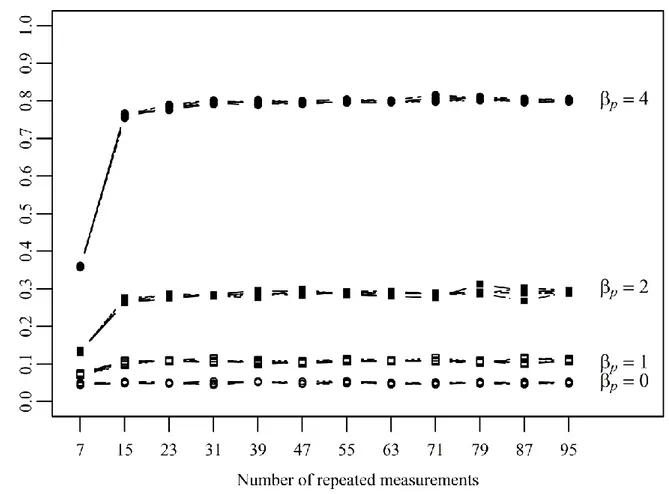
65 Next, we ask questions concerning the power of the t-tests associated with the orthogonal polynomial contrasts (
X
1,…,X
5). Figure 5 shows the empirical power curves for the five t-tests (one test for each polynomial contrast) as a function of effect size ( ) and number of repeated meas-urements (T). Power curves for the five tests are virtuallyidentical because
β
1 =β
2 = … =β
5 . Again, = 0 refers to the empirical Type I error rates which are close to 5% re-gardless of number of time points. Using more than T = 31 points in time does not increase the power of the t-tests. For very large effects (i.e., = 4), T = 15 measurement occa-sions are sufficient to guarantee acceptable power ratesFigure 5. Relative frequencies of rejecting the null hypothesis of separate t-tests as a function of effect sizes and the number of repeated measurements for the single-subject design.
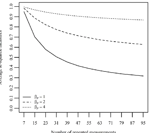
Finally, Figure 6 shows the average R² values of the ANOVA models as a function effect size and number of measurement occasions. Two effects can be observed. First, R² values increase with , as expected. Second, average R² values
decrease with the number of measurement occasions. This result can be explained by the fact that the portion of unex-plained variance increases with the length of the series.
66
Figure 6. Average R² values as a function of effect size and number of measurement occasions for the single-subject design.
Comparison of two series of scores
We now ask questions concerning the power of ANOVA for the question whether two individuals (i.e., n = 2) differ in their trajectories. Data were generated according to the true model
In other words, the design matrix consisted of 12 columns, i.e., a constant vector (representing the intercept
β
0), a vec-tor S consisting of the values 0 and 1 representing the two subjects (withβ
S being the subject effect), five columnsrepresenting the orthogonal polynomial contrasts (with (p = 1,…,5) being the slopes of the five polynomial con-trasts), and five columns defining the Subject × Time
inter-actions. Again, the intercept was fixed at
β
0 = 0 and the slope parameters (i.e.,β
S =β
p= β
Sp with p = 1,...,5) were fixed at 0, 1, 2, and 4.β
S =β
p= β
Sp = 0 refers to the Type I error performance of the ANOVA,β
S =β
p= β
Sp > 0 re-fers to the power of the ANOVA. The numbers of repeated measurements were T = 7, 15,... (8) …, 87, and 95. As in the first simulation, the simulation factors were crossed which resulted in 4 (effect sizeβ
p) × 12 (time points T) = 48 experimental conditions, and for each condition, 5000 samples were generated. Statistical decisions (i.e., retaining or rejecting the null hypothesis) were based on a nominal significance level of 5%. Figure 7 shows the population trajectories for both subjects using 50 measurement occa-sions.67
Figure 7. Population model for the comparison of two series of scores (case A versus case B) for T = 50 measurement oc-casions as a function of effect size.
Table 8 shows the portion of rejected null hypotheses for the overall ANOVA F-test. For zero effects, the rejection rates are close to the nominal significance level of 5%. Empirical Type I error rates are within Bradley's (1978)
strict robustness interval. Further, for
β
p ≥ 1, 15 time points are sufficient to achieve a power larger than 80% which is considered acceptable for the behavioral and social sciences (Cohen, 1988).Table 8
Relative frequencies of rejecting the null hypothesis for the overall ANOVA F-tests when comparing two series of scores.
Time points (T)
β
p = 0β
p = 1β
p = 2β
p = 4 7 0.046 0.165 0.435 0.885 15 0.047 0.884 1.000 1.000 23 0.049 0.968 1.000 1.000 31 0.048 0.990 1.000 1.000 39 0.050 0.997 1.000 1.000 47 0.047 0.999 1.000 1.000 55 0.048 1.000 1.000 1.000 63 0.046 1.000 1.000 1.000 71 0.046 1.000 1.000 1.000 79 0.048 1.000 1.000 1.000 87 0.051 1.000 1.000 1.000 95 0.049 1.000 1.000 1.00068 Next, we analyzed the empirical power curves of the t-tests for the polynomial contrasts. We were particularly interested in empirical power curves for the interaction hy-potheses (the power curves for the main effects of the or-thogonal polynomial contrasts were virtually identical to those given in the single-subject case; see Figure 4). Figure 8
shows the portion of rejected null hypotheses for the Subject × Time interactions. All t-tests keep the nominal signifi-cance level of 5% when
β
Sp = 0. Except for very large ef-fects (β
Sp = 4), the power of the t-tests is rather low. Most important, increasing the number of measurement occasions beyond T = 15 does not affect the power of the tests.
Figure 8. Relative frequencies of rejecting the null hypotheses for testing Subject × Time interactions as a function of effect size and number of repeated measurements.
Finally, Figure 9 shows the average R² values obtained from the generated series of scores. Again, the portion of explained variance increases with the effect size and
de-creases with the number of time points. The latter effect can again be explained by the fact that longer series induce larger portions of unexplained variability
.
69
Figure 9. Average R² values as a function of effects sizes and number of repeated measurements when comparing two series of scores
Discussion
There are many points of discussion that can be elabo-rated based on the six scenarios illustelabo-rated above and the simulation results. Three points stand out. The first is most important from the perspective of person-oriented research: it is possible to estimate individual-specific parameters using such GLM methods as repeated measures ANOVA and regression. Not only can one ask for parameters that describe individual development, one can also ask whether individuals differ in parameters. These parameters can be standard ANOVA contrast parameters, but they can also describe trends and such characteristics of trends as linear, quadratic, or cubic curvature. When trends are estimated, problems with serial dependency will not arise. In either case, the trajectories of individuals can be compared, but also the trajectories of groups of individuals, and once-observed factors and covariates can be made part of an analysis.
The simulation results suggest that there is sufficient
power when the number of observation points is 15 or higher for single subject designs. For the comparison of two individuals, sufficient power begins at 15 observations as well but effects must be stronger. This result mirrors the well-known ANOVA characteristic that there is more power for main effects than for interactions.
The second point of importance is related to the first. As in standard repeated measures ANOVA, not all parameters of interest may be testable in a single run. Therefore, for each run, researchers have to make decisions about how to create degrees of freedom. Parameters can be fixed, set equal, effects can be removed from a model, or any combi-nation of these can be considered. In standard repeated measures ANOVA, the highest-level interaction is removed from the model (most ANOVA software packages do this without even asking the user). Here, we illustrated that oth-er options exist.
The third point that became obvious is that power can be minimal, in particular when the number of observation points is small. We therefore ask how power can be
im-70 proved. In von Eye and Bogat’s (2004) discussion of the use of ANOVA in person-oriented research, one answer was given by operating at the aggregate level, that is, by creat-ing groups of cases. Here, we suggest also considercreat-ing in-creasing the length of the series of measures, thus moving in the direction of creating intensive longitudinal data (Walls & Schafer, 2006) or beyond. This issue was detailed in the simulations presented in the preceding section of this article. Results of the simulations suggest that power rap-idly increases with the length of the series. However, in all scenarios, we also found ceiling effects. That is, increasing the length of a series beyond a critical number of observa-tion points will not further increase power.
Finally, and most important in the context of repeated observations, the issue of dimensional identity (von Eye & Bergman, 2003) needs to be considered. When observa-tional studies are conducted or the same questions are pre-sented repeatedly, the same behavior and the same question may change in meaning over the course of a study. The semantic space, for example, that adolescents use to answer the question why they smoke can be different than the se-mantic space the same individuals use when they answer the same question 10 years later. Therefore, the answers to this question may not be quantitatively comparable over time. Series of scores to answers to questions that can change meaning over time may not be interpretable. All this may be less of an issue when physiological measures such as brain waves, blood pressure, or hormone level are rec-orded over time.
Therefore, a necessary condition for meaningful analysis of series of scores is that dimensional identity obtains. In other words, the scales that are used for repeated observa-tions must have the same psychometric and semantic char-acteristics at each observation point and for each respondent.
References
Abramowitz, M., & Stegun, I. A., (Eds.), (1972), Handbook of
Mathematical Functions with Formulas, Graphs, and Mathe-matical Tables. New York, NY: Dover Publications.
Bergman, L. R., & Magnusson, D. (1997). A person-oriented ap-proach in research on developmental psychopathology.
Devel-opment and Psychopathology, 9, 291-319. doi: 10.1017/S095457949700206X
Bogat, G. A., Levendosky, A. A., DeJonghe, E., Davidson, W. S., & von Eye, A. (2004). Pathways of suffering: The temporal effects of domestic violence on women's mental health.
Maltrattamento e abuso all'infanzia, 6, 97-112.
Bradley, J. V. (1978). Robustness? British Journal of
Mathematical and Statistical Psychology, 31, 144-152.
Brillinger, D.R. (2002). John W. Tukey's work on time series and spectral analysis. Annals of Statistics, 30, 1595-1618.
Chow, S.-M., Witkiewitz, K., Grasman, R., Hutton, R. S., & Maisto, S. A. (2014). A regime-switching longitudinal model of alcohol lapse – relapse. In P. C. M. Molenaar, R. M. Lerner, & K.
M. Newell, (Eds.), Handbook of developmental systems theory
and methodology (pp. 397-422). New York, NY: Guilford Press.
Cohen, J. (1988). Statistical power analysis for the behavioral
sciences (2nd ed.). Hillsdale: Lawrence Erlbaum Associates. Cunha, F. & Heckman, J. (2014). Estimating the technology of
cognitive and noncognitive skill formation: The linear case. In P. C. M. Molenaar, R.M. Lerner, & K.M. Newell, (Eds.),
Hand-book of developmental systems theory and methodology (pp.
221-269). New York, NY: Guilford Press.
Games, P. A. (1983). Curvilinear transformations of the dependent variable. Psychological Bulletin, 93, 382-387. doi: 10.1037/0033-2909.93.2.382
Games, P. A. (1984). Data transformations, power, and skew: A rebuttal to Levine and Dunlap. Psychological Bulletin, 95, 345-347. doi: 10.1037/0033-2909.95.2.345
Hamaker, E. L., Dolan, C. V., & Molenaar, P. C. M. (2005). Statis-tical modeling of the individual: Rationale and application of multivariate stationary time series analysis. Multivariate
Behav-ioral Research, 40, 207-233. doi: 10.1207/s15327906mbr4002_3
Huth-Bocks, A. C., Levendosky, A. A., Bogat, G. A., & von Eye, A. (2004). The impact of maternal characteristics and contextual variables on infant-mother attachment. Child Development, 75, 480-496. doi: 10.1111/j.1467-8624.2004.00688.x
Kirk, R. E. (1995). Experimental design (3rd ed.). Pacific Grove, VA: Brooks/Cole.
Kutner, M. H., Nachtsheim, C. J., Neter, J., & Li, W. (2005). Applied linear statistical models, 5th ed. Boston: McGraw-Hill. McCullagh, P. & Nelder, J.A. (1989). Generalized linear models
(2nd ed.). London: Chapman and Hall.
Molenaar, P. C. M. (2004). A manifesto on Psychology as idiographic science: Bringing the person back into scientific Psychology-this time forever. Measurement: Interdisciplinary
Research and Perspectives, 2, 201-218. doi: 10.1207/s15366359mea0204_1
Molenaar, P. C. M., & Campbell, C. G. (2009). The new person-specific paradigm in psychology. Current Directions in
Psychology, 18, 112-117. doi: 10.1111/j.1467-8721.2009.01619.x
Molenaar, P. C. M., & Nesselroade, J. R. (2014). New trends in the inductive use of relational developmental systems theory: Ergodocity, nonstationarity, and heterogeneity. In P. C. M. Molenaar, R. M. Lerner, & K. M. Newell (eds.), Handbook of
developmental systems theory and methodology (pp. 442-462.
New York, NY: Guilford Press.
Molenaar, P. C. M., Lerner, R. M., & Newell, K. M. (Eds.), (2014). Handbook of developmental systems theory and
methodology. New York, NY: Guilford Press.
Molenaar, P. C. M., & Newell, K. M. (Eds.) (2010). Individual
pathways of change: Statistical models for analyzing learning and development. Washington, DC: American Psychological
Association.
Molenaar, P. C. M., Sinclair, K. O., Rovine, M. J., Ram, N., & Corneal, S. E. (2009). Analyzing developmental processes on an individual level using non-stationary time series modeling.
71 Scheffé, H. (1959). The analysis of variance. New York, NY:
Wiley.
Toothaker, L. E., Banz, M., Noble, C., Camp, J., & Davis, D. (1983). N = 1 designs: The failure of ANOVA-based tests.
Journal of Educational Statistics, 8, 289-309.
Tukey, J. W. (1949). One degree of freedom for non-additivity.
Biometrics, 5, 232-242.
Tukey, J. W. (1961). Discussion, emphasizing the connection between analysis of variance and spectrum analysis.
Technometrics, 3, 191-219.
Van Rijn, P. W., & Molenaar, P. C. M. (2005). Logistic models for single-subject time series. In L. A. van der Ark, M. A. Croon & K. Sijtsma (Eds.), New developments in categorical data
analy-sis for the social and behavioral sciences (pp. 125-145).
Mah-wah, NJ: Erlbaum.
von Eye, A. & Bergman, L.R. (2003). Research strategies in developmental psychopathology: Dimensional identity and the person-oriented approach. Development and Psychopathology,
15, 553 – 580. doi: 10.1017.S0954579403000294
von Eye, A., Bergman, L. R., & Hsieh, C.-A. (2015). Person-oriented approaches in developmental science. In W.F.
Overton, & P.C.M. Molenaar (Eds.), Handbook of child
psychology and developmental science - theory and methods.
New York: Wiley. (in press)
von Eye, A. & Bogat, G. A. (2007). Methods of data analysis in person-oriented research. The sample case of ANOVA. In A. Ittel, L. Stecher, H. Merkens, & J. Zinnecker (Eds.), Jahrbuch
Jugendforschung 2006 (pp. 161-182). Wiesbaden: Verlag für
Sozialwissenschaften.
von Eye, A., Mair, P., & Mun, E.-Y. (2010). Advances in
Configural Frequency Analysis. New York, NY: Guilford Press.
von Eye, A. & Mun, E.-Y. (2013). Log-linear modeling -
Concepts, Interpretation and Applications. New York, NY:
Wiley.
von Eye, A. & Schuster, C. (1998). Regression analysis for social
sciences - models and applications. San Diego, CA: Academic
Press.
Walls, T. A., & Schafer, J. L. (Eds.), (2006), Models for Intensive
Longitudinal Data. Oxford, UK: Oxford University Press.
Winer, B.J. (1970). Statistical principles in experimental design. New York, NY: McGraw-Hill.