Department of Wildlife, Fish, and Environmental Studies
Variations in nutritional content of key
ungulate browse species in Sweden
Leonardo Capoani
Master´s thesis • 60 credits
Management of Fish and Wildlife Populations Examensarbete/Master's thesis, 2019:15 Umeå 2019Variations in nutritional content of key ungulate browse species
in Sweden
Leonardo Capoani
Supervisor: Joris Cromsigt, Swedish University of Agricultural Sciences, Department of Wildlife, Fish, and Environmental Studies
Assistant supervisor: Robert Spitzer, Swedish University of Agricultural Sciences, Department of Wildlife, Fish, and Environmental Studies
Assistant supervisor: Annika Felton, Swedish University of Agricultural Sciences, Southern Swedish Forest Research Centre
Examiner: Wiebke Neumann, Swedish University of Agricultural Sciences, Department of Wildlife, Fish, and Environmental Studies
Credits: 60 credits
Level: Second cycle, A2E
Course title: Master Thesis in Biology, A2E – Management of Fish and Wildlife Populations – Master’s Programme
Course code: EX0935
Programme/education: Management of Fish and Wildlife Populations
Course coordinating department: Department of Wildlife, Fish, and Environmental Studies
Place of publication: Year of publication: Cover picture: Title of series: Part number: Online publication: Keywords: Umeå 2019 Leonardo Capoani Examensarbete/Master's thesis 2019:15 https://stud.epsilon.slu.se
Ungulate diet, cervids, nutrition, browsing, Sweden, NIR, NDF, protein
Swedish University of Agricultural Sciences Faculty of Forest Sciences
Understanding variations in the nutritional content of key ungulate browse species is not an easy task. Overall, my study focused to understand seasonal variations in nutritional values, available to wild browsers, found in the main tree and shrub species present in Scandinavia. Water, neutral detergent fibre (NDF) and crude protein (CP) content of twelve different plant species (i.e. 8 belongs to tree whilst 4 to shrub) collected in two different location of Sweden were analysed. My experiment produced five main key findings. Firstly, overall seasonality variation was recorded in all three nutritional components analysed; CP and water decreased from summer to winter, whereas NDF increased. Broadleaved species were more affected than evergreen species. A different situation was found for evergreen, where the seasonal variation recorded was very small for some species (e.g. CP in pine and NDF in spruce) and non-existing for others (e.g. lingonberry, Labrador tea and juniper). Secondly, the seasonal NDF-CP ratio showed a negative correlation between the two nutrients only for broadleaf, while for evergreen species the seasonal NDF-CP ratio was not significant. Thirdly, most of the high protein content was primarily found in leaves of broadleaved species during the vegetative season. During winter, however, pine and Labrador tea showed higher values for CP than the ones found in broadleaved twigs. The fourth finding showed whether for some species the twig size affected the NDF and CP levels. Aspen, silver and downy birch increased their protein content with the increase of the diameter, while aspen, salix, rowan and silver birch raised the NDF levels with the increase of the twigs’ diameter. Finally, the fifth result concerned the habitat and latitude effect. No significant effect of habitat onto NDF and CP was found, while latitude affected water content and CP but not NDF.
Keywords: Ungulate diet, cervids, nutrition, browsing, Sweden, NIR, NDF, protein Abstract
List of tables: ... 4
List of figures ... 5
List of appendix ... 7
Abbreviations ... 9
1 Introduction ... 11
1.1 Aims and objective ... 14
2 Material and method ... 15
2.1 Location of the study area ... 15
2.2 Experimental design ... 15
2.3 Data collection and first-round ... 17
2.4 Sample preparation and hyperspectral imaging ... 18
2.5 Wet chemical analysis ... 19
2.6 Estimation of nutrition traits with hyperspectral images ... 20
2.7 Statistical analysis... 20
3 Results ... 22
3.1 Seasonality of CP, NDF and H2O ... 22
3.2 Nutritional value in leaves, twigs, and twigs with leaves ... 26
3.3 Effect of latitude and habitat... 27
3.4 Twig size ... 29
4 Discussion ... 31
Contents
4.1 Seasonality and latitudinal effect on nutritional content ... 31
4.2 Browsing options and their nutritional values ... 34
4.3 Habitat effect ... 35 4.4 Study limitation ... 35 5 Conclusion ... 37 Acknowledgement ... 38 References ... 39 Appendix ... 45
4
Table 1: List of the species of boreal trees and shrubs collected during the study, and their specific conversion factors that can be used to calculate a rough estimate about the amount of dried matter obtained from 1 gram of fresh material. These values here reported are based on the water content in each item. Note that each broadleaf’s species present 2 values (i.e. one for leaves during the vegetational season and one for twigs measured through the 4 season) while the evergreen species figure one value (i.e. obtained by the twigs and leaves together), due to the portion of the plant consumed by browsers. ... 16 Table 2: Seasonal mean values (± standard deviation) of H2O, CP and NDF, for each species analysed ... 22
List of tables:
5
Fig. 1: Redrawn classification made by Hofmann (1989), of wild (dark) and domesticated (white) ungulate species existing in Sweden (van Wieren, 1996, Staaland et al., 1997, Vera, 2000). The even-toed ungulates are divided into two categories depending on the digestive physiology: ruminant (foregut fermentation) and non-ruminant (hindgut fermentation). Further subdivision within the groups is made following the food preferences and feeding behaviour of each species (i.e. browsers, intermediate feeders and grazers). ... 12 Fig. 2: Optimals RMSE (root-mean-squared error) and number of components stored in the bestmodels. The costFuncGraphs shows how the models were built, where the green dots indicate the lowest RMSE value, avoiding overfitting. ... 20 Fig. 3: Seasonal change in water content in 4 different groups. The groups here listed are broadleaved shrubs (bilberry) and trees (aspen, rowen, birches and Salix), evergreen trees (pine, spruce and juniper) and shrubs (lingonberry, header and Labrador tea). ... 23 Fig. 4: Seasonal change in protein content in 4 different groups. The groups here shown are broadleaved
shrubs(bilberry) and trees (aspen, rowen, birches and Salix), evergreen trees (pine, spruce and juniper) and shrubs (lingonberry, header and Labrador tea). ... 24 Fig. 5: Seasonal change in NDF content in 4 different groups. The groups here shown are broadleaved
shrubs(bilberry) and trees (aspen, rowen, birches and Salix), evergreen trees (pine, spruce and juniper) and shrubs (lingonberry, header and Labrador tea). ... 25 Fig. 6: Linear relationship between NDF and CP in broadleaved (on the left side) and evergreen (on the right side) species. The broadleaved plants (aspen=As, rowan=Ro, Salix=Sal, silver birch=SB, downy birch=DB, bilberry=Bb) showed a negative correlation between NDF and crude protein throughout the year (r =0.62, p ≤0.01). On the other hand, no relationship (p=0.37) between the two nutritional components was found in evergreen species (heather=Cal, lingonberry=L, Labrador tea=Lt, juniper=J, pine=Pi, spruce=Sp). ... 25 Fig. 7: Monthly change in CP among the samples’ components in each species (aspen=As, rowan=Ro, Salix=Sal, silver birch=SB, downy birch=DB, bilberry=Bb, heather=Cal, lingonberry=L, Labrador tea=Lt, juniper=J,
6
pine=Pi and spruce=Sp). Plants were grouped based on the browser’s behaviour: both (i.e. include leaves and twigs for evergreen trees, shrubs and broadleaved shrubs), twigs and leaves (i.e. categories obtained by the separation of samples collected from broadleaved trees). ... 26 Fig. 8: Monthly change in NDF among the samples’ components in each species (aspen=As, rowan=Ro,
Salix=Sal, silver birch=SB, downy birch=DB, bilberry=Bb, heather=Cal, lingonberry=L, Labrador tea=Lt, juniper=J, pine=Pi and spruce=Sp). Plants were grouped based on the browser’s behaviour: both (i.e. include leaves and twigs for evergreen trees, shrubs and broadleaved shrubs), twigs and leaves (i.e. categories obtained by the separation of samples collected from broadleaved trees). ... 27 Fig. 9: Habitat effect on protein content, for all the 12 species sampled(aspen=As, rowan=Ro, Salix=Sal, silver birch=SB, downy birch=DB, bilberry=Bb, heather=Cal, lingonberry=L, Labrador tea=Lt, juniper=J, pine=Pi and spruce=Sp). Habitat type here listed are clear-cut planted (CCp), coniferous mixed forest (CFm), coniferous pine forest (CFp), coniferous spruce forest (CFs), deciduous forest (DF), edge (E), mire (M), mixed forest (MF) and road edge (R). ... 28 Fig. 10: Habitat effect on NDF content, for all the 12 species sampled(aspen=As, rowan=Ro, Salix=Sal, silver birch=SB, downy birch=DB, bilberry=Bb, heather=Cal, lingonberry=L, Labrador tea=Lt, juniper=J, pine=Pi and spruce=Sp). Habitat type here listed are clear-cut planted (CCp), coniferous mixed forest (CFm), coniferous pine forest (CFp), coniferous spruce forest (CFs), deciduous forest (DF), edge (E), mire (M), mixed forest (MF) and road edge (R). ... 29 Fig. 11: Relationship between protein content and average twig diameter, among different species. ... 29 Fig. 12: Relationship between fibre content and average twig diameter, among different species. ... 30
7
Appendix 1.1: Location of the two different reference areas. The northern one is Nordmaling (NM) about 50 km South-West of Umeå, while the southern one is Öster Malma (ÖM) approximately 90 km South-West of Stockholm. ... 45 Appendix1.2: FOMA tracts in the Nordmaling reference area (left) and tract layout with examples of circular samples areas, with 10m radius, in red (right). ... 46 Appendix 1.3: The map shows Öster Malma area and reports the corresponding FOMA (fortlöpande
miljöanalys) monitoring number, that I have chosen as representative transects for this sampling site. ... 46 Appendix 1.4: The map shows Nordmaling area and reports the corresponding FOMA (fortlöpande miljöanalys) monitoring number, that I have chosen as representative transects for this sampling site. ... 47 Appendix 2.1: Field sheet’s frame used for Nordmaling and Öster Malma data collection. Both sheets present three main sections. On the top I can find all the general information (i.e. name of the collector, date, number of the tract which is sampled in a specific occasion, and season). In the middle part there is all the specific information regarding the sample collected during a single round (i.e. sample number according to the rule explained in Chapter 2.4., spaces to cross when the sample and the waypoint the , and spaces to be able to write the habitat type and eventually remarks). The third and last part contains all the specifications necessary for the collector to complete the two sections above, plus a checking list for the first round of collection. . 48 Appendix 3.1: This table summarizes the habitat types for the species collected in each tract, detected during the first round of data collection in Nordmaling area. ... 50 Appendix3.2: The table summarizes the habitat types for the species collected in each tract, detected during the first round of data collection in Öster Malma area. ... 50 Appendix3.3: Proportion of sample collected per each species was unequal among different habitat types.
Habitat types are clear-cut planted (CCp), coniferous mixed forest (CFm), coniferous pine forest (CFp), coniferous spruce forest (CFs), deciduous forest (DF), edge (E), mire (M), mixed forest (MF) and road edge (R). the species here listed are: aspen=As, rowan=Ro, salix=Sal, silver birch=SB, downy birch=DB, bilberry=Bb, heather=Cal, lingonberry=L, labrador tea=Lt, juniper=J, pine=Pi and spruce=Sp. ... 51
List of appendix
8
Appendix 4.1: Monthly average of the relative humidity in the two study sites: Oster Malma (Floda A meteorological station) and Nordmaling (Järnäsklubb meteorological station). Data provided by https://www.smhi.se/data. ... 52 Appendix 4.2: Monthly rainfall recorded in the two study sites: Oster Malma (Floda A meteorological station) and Nordmaling (Järnäsklubb meteorological station). Data provided by https://www.smhi.se/data... 52 Appendix 4.3: Monthly average of the air temperature in the two study sites: Oster Malma (Floda A
meteorological station) and Nordmaling (Järnäsklubb meteorological station). Data provided by https://www.smhi.se/data. ... 53
9
Chemical analysis:
CP Crude protein
DM Dried matter (the moisture-free component of the sample)
NDF Neutral detergent fibre (insoluble fibre represented by cellulose, hemicellulose and lignin) Trees and shrubs species:
Pi Sp SB DB Ro As Sal J Bb L Cal Lt
Pine (Pinus sylvestris) Spruce (Picea abies)
Silver birch (Betula pendula) Downy birch (Betula pubescens) Rowan (Sorbus aucuparia) Aspen (Populus tremula) Willow spp. (Salix spp.) Juniper (Juniperus communis) Bilberry (Vaccinium myrtillus) Lingonberry (Vaccinium vitis-idea) Heather (Calluna vulgaris)
Labrador tea (Rhododendron tomentosum) Generic terms:
NM Nordmaling area
ÖM Öster Malma area
Tract It refers to an area; e.g. there are 5 tracts (each 1x1km) in the Öster Malma and other 5 tracts in the Nordmaling reference area.
Transect It refers to a line; e.g. the outer borders of a 1x1km tract form a 4 km transect.
Twig The small and thin terminal branch section of a woody plant (i.e. in this specific case I consider twigs branches with a maximum diameter of 4 mm)
11
Human attitudes towards wildlife started to change in the late nineteenth and beginning of the twentieth century, primarily with increasing awareness regarding the value of game species of large ungulates within the society (Putman et al., 2011). At the same time, change in human land-use practices and harvesting strategies, reintroduction, restoration of habitat, and decline in abundance of natural predators, boosted ungulate abundance in Europe (Jędrzejewski et al., 2010). This resulted in an important impact on the vegetation, due to their selective browsing on tree, shrub and grass species (Apollonio et al., 2010). Likewise, a similar situation has been seen in Sweden and Norway, where the increase in abundance of large herbivores, combined with development in forestry practices and rise in the economic interest of forest industry, has resulted in relatively high levels of forest damage in both the temperate and boreal forests (Herfindal et al., 2015). Nowadays, four wild species of even-toed ungulates belonging to the Cervidae family are present on the Scandinavian peninsula: roe deer (Capreolus capreolus), red deer (Cervus elaphus), fallow deer (Dama dama), moose (Alces alces), and one species of semi-domesticated ungulate, the reindeer (Rangifer tarandus) (Apollonio et al., 2010, Liberg et al., 2010). Wild herbivores have a common strategy for processing plant tissues, which have high concentrations of cellulose and hemicellulose. Specifically Cervidae, thanks to their gastrointestinal structure being well developed, are able to utilize high cellulose containing plant material such as leaves, bark and woody twigs, through an efficient digestive process (Tajchman et al., 2018, Shipley et al., 1998, Van de Veen, 1979, Belovsky, 1981). These polysaccharides are unavailable to most of the vertebrates because of the inability of their endogenous digestive-enzymes to extract nutrients (Stevens and Hume, 2004, Langer, 1988). However, cervids and other ruminants, use the symbiosis existing with cellulase-producing microorganisms to ferment and degrade fibrous food sources, allowing thus nutritive component to be extracted and digested from food sources. These microorganisms have also another important function in the rumen that consist of synthesizing microbial protein, degrading dietary and endogenous protein (Stern et al., 2006). Microbial protein synthesis is highly efficient, providing between 50 and 80% of total absorbable protein. Therefore animal must introduce into the rumen enough quantity and quality of dietary protein (Stern et al., 2006, Klein and Schønheyder, 1970).
Thus, to be able to meet their requirements, cervids must select the habitat where the plants grow, plant taxa, and plant parts (Alldredge et al., 2002, Vivås et al., 1991). Based on their selectiveness and food preferences, Hofmann (1985) categorized ruminants in different classes looking at feeding strategy and structure of the
12
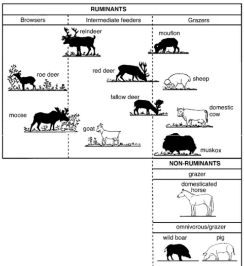
digestive system. Accordingly, it is possible to divide wild ruminant into three major groups (Fig. 1): concentrate feeders (or browsers), intermediate feeders and specialized grass eaters (or grazers).
Fig. 1: Redrawn classification made by Hofmann (1989), of wild (dark) and domesticated (white) ungulate species existing in
Sweden (van Wieren, 1996, Staaland et al., 1997, Vera, 2000). The even-toed ungulates are divided into two categories depending on the digestive physiology: ruminant (foregut fermentation) and non-ruminant (hindgut fermentation). Further subdivision within the groups is made following the food preferences and feeding behaviour of each species (i.e.
browsers, intermediate feeders and grazers).
When the two extreme groups are analysed, browsing differs from grazing mainly on the food category eaten. In fact, for the first group, the diet is mostly represented by woody and non-woody dicotyledonous plants, whilst grazers feed mainly on grasses (Gordon and Prins, 2008). Other aspects can also be considered in this classification, such as digestive system morphology and physiology (Fletcher et al., 2010, Hofmann, 1985, van Wieren, 1996), and foraging behaviour in terms of the relationship between intake rate and resource abundance (asymptotic in grazers and linear in browsers) (Gordon and Prins, 2008).
From a theoretical framework perspective, each food item present in the diet can be seen as a trade-off between quality (e.g. digestibility, macro and micronutrients), which can vary during different time-period (such as seasons) and quantity of food that can be ingested (Moen et al., 1997). Generally speaking, it has been suggested
13
that free-ranging intake (Belovsky, 1981, Barboza et al., 2008). Therefore, feeding strategies are needed to maximize the capture rate of some nutrient, which seems to be mainly driven by specific macro and micro-nutrients requirement, and strictly related to age, sex and physiological phase (i.e. antler development for males and lactation for females) (Tajchman et al., 2018, Robbins, 2012). Recently, a study done by Felton et al. (2016), perfected a previous theory on "optimization model" for diet selection by Large Generalist Herbivores created by Westoby (1974). They observed that captive-moose do not seem to maximize their nutritional intake of energy but rather finding a nutritional balance under specific environmental circumstances; the so-called nutrient balancing hypothesis. Furthermore, most of the studies done on wild deer diet mainly focused on one or few tree/s or shrub/s species or one or few nutritional component/s, missing in this way the linkage between nutritional aspect and the observed diet (i.e. mitochondrial DNA analysis on faeces or ruminal content) (Felton et al., 2018). So where are the main nutrients, available to the browsers, found in the trees and shrubs? Looking at the plant anatomy, plant tissues are composed of water and dry fraction, which is also called dry matter (DM). Once the water is extracted, the DM can be further divided into organic matter (OM) that includes all the combustible material, which is primarily based on carbon (C), nitrogen (N), hydrogen (H) and oxygen (O), and the non-combustible fraction (ash) that includes most of the minerals. The three main structures composing OM are protein, carbohydrates (both structural (fibres) and non-structural (sugars and starches)) and lipid (Barboza et al., 2008).
Protein is principally stored in protein storage vacuoles of terminally differentiated cells of the embryo or endosperm, and as protein bodies. They are typically found in seed and fruit, inducing the growth of vegetative organs after the dormancy (Herman and Larkins, 1999). Therefore, N storage is strongly related to tree phenology, showing seasonal variation due to source remobilization and the tissue´s stage development (Millard and Grelet, 2010). This can be explained through investigation in the concept of N storage. It has been shown that the ability to accumulate or store N is not dependent on the external supply but it is strongly related to the phenological event that requires N such as shoot growth, maintenance and defence (Millard, 1988, Miller, 1986). Usually, the protein storage can be reutilized by the plant, even though exist some situations (as an example found in the pine needles) where the plant seems to be non-capable in reusing or withdrawing deposit of N (i.e. pine needles), once the storage is created (Näsholm, 1994).
In contrast, trees can accumulate large amounts of C as non-structural carbohydrates (NSC) and lipids with profound differences if compared to the scarce seasonal allocation of N. Vascular plant produce a range of soluble and insoluble carbohydrates through the well-known photosynthetic process happening in the leaf (Wardlaw, 1968). Once monosaccharides are produced, several units (from two to ten) are linked together in different ways by glycosidic bonds, creating chains so-called di-, tri-, tetra-, […], oligo- or poly- saccharides. Generally, most of the carbohydrates with storage function in plants are figured by polysaccharides, such as starch, hemicellulose and pectin (Lewis, 1984a). The first two polymers can be found in different proportions between different species, parts of the plant and daily phases of the photosynthetic cycle (Lewis, 1984b). Whilst, pectin together with hemicellulose constitute the basic component for the cell-wall, generating fibrillar polysaccharides, commonly
14
known as cellulose (Lewis, 1984a). Cell walls are thickened and strengthened subsequently with a complex phenolic polymer called lignin.
Thus, for a better understanding of the wild Cervids’ diet and to inspect different ideas on feeding strategy, I decided to focus on the nutritional values of several species of plants, which will be used to link it to Cervids diet composition in further study.
1.1 Aims and objective
My study primarily concerns the assessment of the nutritional "quality" of important forage plants for cervids and understand how this quality changes throughout the year. There are many different ways to measure nutritional components that are relevant with regards to forage quality. In this study, I will only focus on water (H2O) and two organic compounds, which can be used as reasonable indicators for the quality of the available
browse (Christianson and Creel, 2015, González-Hernández and Silva-Pando, 1999): CP and NDF content. My objective was to study the seasonal pattern in crude protein and NDF in a total of twelve species of shrubs and trees, representing the main resources of forage for browsers and intermediate feeders in the boreal forest. The output of this study will be used (in another research project not yet published) to understand nutritional dynamics and specific feeding strategies of free-ranging moose, roe-, fallow- and red- deer (and occasionally reindeer). According to the literature, I hypothesized that:
I. Water content changes through the seasons differently within the deciduous tree/shrubs than within coniferous evergreen trees/shrubs;
II. Seasonal variation in CP and NDF content should be consistent in all species;
III. CP is found in higher concentration in leaves if compared to twigs during the vegetative season (linked to plant phenology).
IV. Habitat type has an influence on NDF and protein content;
V. Relationship between NDF and Protein is different regards on the belonging plant’s groups (i.e. broadleaves or evergreen);
VI. At an equal length of the twigs, twig diameter size positively affects CP content of twigs, due to plant’s vigour.
15
2.1 Location of the study area
The study was carried out between the 29th May 2018 and 10th February 2019 focused in two sampling sites in
Sweden, located in Nordmaling (63°34'07"N, 19°30'23"E) and Öster Malma (58°57'07.6"N 17°09'25.4"E) (Appendix 1.1). The climate is different in the two study areas, where the northern one is bordering on a humid continental and a subarctic climate, with short and fairly warm summers with average temperature not higher than 25 °C, but long and cold winter (Beck et al., 2018). While the southern area has a relatively mild-humid continental climate with the mean winter temperature slightly below zero and at least four months whose mean temperatures are at or above 10 °C (Beck et al., 2018). Partly due to the geographic-climatic factors operating in the South, soil fertility and composition, the forest community is different in the two study areas. In fact, according to Diekmann (1994) in the northern area study, the forest is classified as boreal, while in the southern area the forest is boreo-nemoral due to also at the higher presence of deciduous tree species.
2.2 Experimental design
The experimental design was built up around the FOMA (“fortlöpande miljöanalys”, English: environmental monitoring and assessment) monitoring system, set from the Swedish University of Agriculture Science (SLU) with the purpose of long-term follow-up of the state of natural resources. The main reason for choosing this layout is the possibility of allowance a direct linkage with previous studies (e.g. pellet count of ungulates) and ongoing monitoring projects (i.e. such as food availability for browsers and ungulate diet along gradients of land-use and species community composition) done in the same areas.
The design was then structured following these guidelines:
‐ 2 reference areas (i.e. Nordmaling and Öster Malma, mentioned in Chapter 2.1);
‐ 5 sampling sites per study site, for a total of 10 (i.e. 5 in NM and 5 in ÖM), hereafter referred to as ‘tracts’ (see Appendix 1.2). Each sampling tract was chosen from a subset of already existing 1x1 km square-tracts (i.e. which is equal to a 4 km tract) that were established as part of FOMA. These tracts
16
have been chosen based on previous projects done regarding ungulate diet, allowing us to possibly link them;
‐ Every month, during each sample occasion I aimed to collect on all 10 tracts, along a 4 km transect were collected at least 50 g of apical portion such as twigs, buds, leaves, flowers and berries (i.e. depending on the season and species) from 12 different plant species, whom 8 belongs to tree whilst 4 to shrub species (Table 1).
The 12 species here selected, represent the most abundant (i.e., frequent) plant species present in both study areas (Rydin et al., 1999), and are categorized such as the most preferred and important food items for Cervids in the Scandinavian peninsula, as recorded from previous studies.
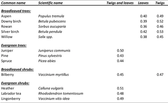
Table 1: List of the species of boreal trees and shrubs collected during the study, and their specific conversion factors that can be
used to calculate a rough estimate about the amount of dried matter obtained from 1 gram of fresh material. These values here reported are based on the water content in each item. Note that each broadleaf’s species present 2 values (i.e. one for leaves during the vegetational season and one for twigs measured through the 4 season) while the evergreen
species figure one value (i.e. obtained by the twigs and leaves together), due to the portion of the plant consumed by browsers.
In fact, studies done on diet selection of moose and roe deer, in the northern coastal Sweden as well as in Grimsö, found that the most favourite plant species were Scots pine (Pinus sylvestris) and willow (Salix spp.), while secondly were also consumed other species such as common juniper (Juniperus communis), rowan (Sorbus aucaparia), aspen (Populus tremula), birches (Betula spp.) (Shipley et al., 1998, Månsson et al., 2007, Cederlund, 1980). Within draft shrubs, bilberry (Vaccinium myrtillus), lingonberry (Vaccinium vitis-idea) and heather (Calluna vulgaris) seem to be the preferred species (Bergquist et al., 1999). Differently from moose, roe deer feed also on Norway spruces (Picea abies), especially on seedling planted trees (Bergquist and Örlander, 1998).
Common name Scientific name Twigs and leaves Leaves Twigs Broadleaved trees: Aspen Populus tremula 0.40 0.49 Downy birch Betula pubescens 0.39 0.52 Rowan Sorbus aucuparia 0.36 0.46 Silver birch Betula pendula 0.42 0.53 Willow Salix spp. 0.38 0.45 Evergreen trees: Juniper Juniperus communis 0.50 Pine Pinus sylvestris 0.43 Spruce Picea abies 0.44 Broadleaved shrubs: Bilberry Vaccinium myrtillus 0.45 0.47 Evergreen shrubs: Heather Calluna vulgaris 0.51 Labrador tea Rhododendron tomentosum 0.48 Lingonberry Vaccinium vitis‐idea 0.49
17
Due to the recent populations' expansion, not many studies have been done in Sweden on red deer and fallow deer diet. However, we can say that in Europe red deer browse mainly Calluna and Vaccinium, as well as leaves of deciduous trees and conifers (Gebert and Verheyden‐Tixier, 2001), while fallow deer prefer rowan and oak (Quercus spp.) (Moore et al., 2000).
To standardize the sample collection and simulate the browsing action I decided that vegetation must be collected between the ground level up to 130 cm, considered as roe deer feeding-height threshold (De Jong et al., 1995, Gill, 1992, Partl et al., 2002). This decision was based on the fact that roe deer is the smallest Ungulate of all the species included in this study case, therefore I did not want to include samples collected to a height major than this.
Furthermore, to avoid repetitive sampling on one singular plant we set up a rule, where the samples (leaves, twigs, flowers and/or berries) must have been collected from several individual plants within a maximum 10 m distance from the transect. Once the first plant was found, all the other plants must have been within a maximum 10 m radius from this point (A ~ 314 m2, r = 10m) (Appendix 1.2).
In addition, we decided to collect no more than three species per each sampling location (i.e. 10 m radius) but having different collection sites in each tract. In this way we were able to capture several habitat types, avoiding sample’s dependency to a specific location.
During the first collection, I followed the FOMA transect, starting from its closest point to a road. Then, I walked the transect clockwise and each time I came across one of the 12 species, the sample was collected, the locations and habitat type recorded, allowing us to come back every time in the same location. The following times I collected the fresh material from the same habitat but from different plants, avoiding to simulate a re-browsed action.
To guide our collection of plant material I used published information on moose browsing behaviour. I chose moose as a reference for two reasons: i) it is the most studied Cervids in Sweden, so I was able to collect enough information regarding the action of browsing; ii) when looking at the Cervid community living in the two study areas, moose (together with roe deer) is the species categorized as true browser (Hofmann, 1989).
Based on previous studies we decided to collect, for all the 12 species, only the terminal 10 cm of living twigs with the diameters of less or equal to 4 mm. In fact, according to Vivås et al. (1991) and Spaeth et al. (2002), the optimal twig’s diameter for moose is around 4 mm, even though the bite’s size can range from 2 to 8 mm (Shipley et al., 1998).
2.3 Data collection and first-round
The data collection of vegetation samples was done at the end of every month. Because of the time required to walk 4 km transect 5 times, the fieldwork needed at least two working days every month, which were done as close as possible to prevent possible changes in nutritional value between different days. Plant samples were stored in zip-loc plastic bags labelled with a unique ID.
18
All the information regarding the samples were annotated on a pre-printed field sheet (see Appendix 2).
Furthermore, depending on the season the samples looked differently. In fact, in Summer the samples consisted mainly in newly grown twigs, while in winter for broadleaved trees we had only twigs with the absence of leaves. The first-round collection was performed (May 2018) with the intention of capturing, for each tree and shrub species here considered, as many habitat types as possible to acquire the variation in nutrition values (e.g. collect bilberry from a clear-cut in the first tract, while in the next one perhaps from a pine forest, and so on).
After the first round of field collections, we were able to find in Nordmaling all the species except for Aspen in one tract (see Appendix 3.1 and 3.2). On the other hand, a slightly different situation was found in Öster Malma whether heather was absent in one tract, downy birch and rowen in two tracts, and Labrador tea in four (out of five) tracts.
2.4 Sample preparation and hyperspectral imaging
At the end of every tract, the samples were immediately stored in coolers (containing ice packs) to prevent deterioration of the organic material. At the end of the day, all the samples were transferred to a freezer, where the temperature was kept constant at -20°C.
In total 970 samples were collected. The samples remained frozen until the beginning of February. Afterwards, the frozen samples were firstly weighted (and the value recorded as “fresh weight”), the diameter of the terminal section of 3 twigs randomly picked was measured, then every sample was relabelled and dried in a ventilated oven (Memmert UF 750 plus) for 48 hours at a constant temperature of 60°C (Krizsan and Huhtanen, 2013). Due to difficulties to find on the literature some conversion factor (see Table 1) for calculating DM from the fresh material weight regarding tree and shrubs species, I decided to provide an informative table with conversion values based on my measurements.
Subsequently, the dried samples were weighted (i.e. recoded as dry matter) and then grounded with 1.0 mm mesh screen (Krizsan and Huhtanen, 2013) through a laboratory cutting mill (Retsch SM 200). Considering that broadleaved species during the vegetative season present leaves on yearly twigs, they provide a wide opportunity of food selection for browsers that might target differently leaves and twigs (i.e. ungulates species and individuals’ preferences). For example, in accordance with Stolter et al. (2013) mosse consume plenty of twigs during the winter, whereas in summer they seem to be avoided, stripping only the leaves from the twigs. Therefore, I decided to separate leaves from twigs having so 2 different ground fractions belonging to the same species.
Once the samples were processed, the obtained ground product was stored in labelled plastic jars. Finally, all the samples were scanned using a push broom Specim SWIR 3 Hyperspectral Camera with a 15 mm lens and two halogen lamps. The acquired images consisted of 288 spectral bands ranging from 935 to 2457 nm, with a spectral resolution of 12 nm and a spatial resolution of approximately 0.42 mm. The hyperspectral images were collected and analysed with Breeze software (Prediktera, Umeå). All pixels that did not consist of vegetation material were
19
removed from the image using a threshold for three specific wavebands (I think it would be good to add a figure of spectrum here). Finally, a principal component analysis (PCA) model was applied to the images to select a subsample of 300 measurements that covered the whole range of spectral variability of the samples’ population. These samples were then sent to the laboratory for wet chemistry analyses.
2.5 Wet chemical analysis
Wet chemistry analysis was carried out by the DiaryOne lab in the United States according to their protocols (here summarized).
According to González-Hernández and Silva-Pando (1999) parameters like crude protein (CP) and fibre content can be used as a good estimator for food quality. In fact, it has been shown that fibre quality highly affects the rumen microbial requirements and their activity providing energy (Van Soest et al., 1991a), while protein is an essential component in the deer diet (Nagy et al., 1969, Bayoumi and Smith, 1976).
In order to be able to measure the fibre content in a feed, it is possible to use NDF (Neutral Detergent Fibre), which measure all the insoluble fibre represented by cellulose, hemicellulose and lignin as major components (Van Soest et al., 1991b). On the other hand, the most common way of measuring protein it is done indirectly by measuring the total nitrogen content through the Kjeldahl, Dumas or combustion method (Rhee, 2001). Furthermore, in studies with fairly large sample size, as the one here presented, to be able to contain costs and facilitate the process to determine NDF value and protein content, is the use of NIRS (Near-infrared spectroscopy). This recent technology, integrated with wet chemical analysis, has been shown to be a highly trustable method of predicting NDF and CP values (Castro, 2002, Undersander, 2006).
Total N was then determined by combustion using a CN628 (Carbon/Hydrogen/Nitrogen Determinator with loader), an instrument with a furnace containing only pure oxygen, producing combustion (oxidation) once exposed to the sample. The amount of protein was calculated by multiplying the total (N) by the nitrogen to protein conversion factor (6.25) for forages (Chang and Zhang, 2017), considering that the average nitrogen content of proteins was found to be about 16 per cent (1/0.16 = 6.25).
aNDF (amylase and sodium sulphite treated Neutral Detergent Fibre) value was measured with ANKOM technology method based on NDF in feeds with “filter bag technique”. Firstly, the samples are needed to be dissolved from the structural components in plant cells (i.e. pectin, protein sugars and lipids). This measurement consists of immerging samples individually weighed at 0.5g into filter bags and digested for 75 minutes as a group of 24 in 2L of NDF solution in 4 ml Alpha-Amylase and 20g sodium sulphite are added at the start of digestion. Samples are then rinsed three times with boiling water for 5 minutes. Finally, four ml Alpha-Amylase is added to the first two rinses. Water rinses are followed by a 3-minute acetone soak and drying at 105°C for 2 hours (Van Soest et al., 1991b).
20
2.6 Estimation of nutrition traits with hyperspectral images
Partial least square regression (PLSR) models were adjusted to link the hyperspectral measurements with the results of the wet chemistry analyses. PLSR is a method that is particularly sound for investigating data with a large number of and potentially highly correlated explanatory variables (in this case, the 288 bands of the hyperspectral images). The general idea of PLSR is to extract the variables that are the most important to describe the variance of the samples, the so-called latent variables (Tobias, 1995). A precise description of the algorithm used with PLSR can be found in Geladi and Kowalski (1986).
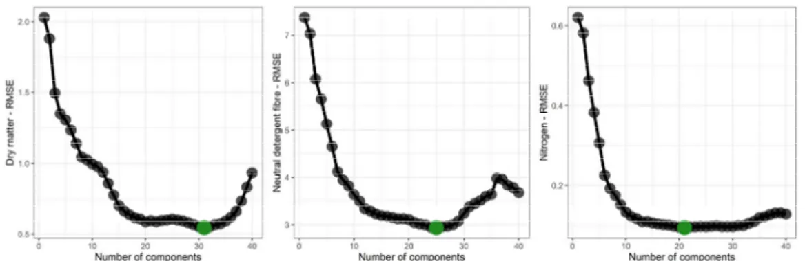
Using the subsampled 300 measurements, PLSR models were adjusted with a leave-one-out cross validation (LOOCV). This method is particularly useful when no testing dataset (i.e., completely independent dataset) is available. The principle of the LOOCV is to run as many calibration and validation rounds as the dataset contain samples. For each of these rounds, one sample will be used for estimating the validation error, while the remaining ones are used to calibrate the model. The averaged sum of the validation errors finally gives the overall error of the model. The number of latent variables used to build the model was optimized to avoid overfitting using the results of the LOOCV (Fig. 2).
Fig. 2: Optimals RMSE (root-mean-squared error) and number of components stored in the bestmodels. The costFuncGraphs
shows how the models were built, where the green dots indicate the lowest RMSE value, avoiding overfitting.
2.7 Statistical analysis
Once the dataset was completed, the hypotheses were tested using linear mixed-effect (lme) or generalized linear mixed-effects model (glmer), depending on the sample and error distribution of the different variable measured (i.e. water, aNDF and Protein). Tract was used as random factor, for the simple reason that even though the samples were collected every occasion from different plants (i.e. independency of the samples), the collection happens repeatedly in the same area of the tract. Doing so I assumed that the tract-specific effect is uncorrelated with the independent variables. Thus, when the analysis were done at species resolution, I accounted for 10 measurements (5 tracts in OM and 5 in NM) per each species, every month. It is also important to consider that most of the analyses were done with a seasonal resolution; including at least 2 months per season.
21
The normality of the sample and error distribution was achieved with the use of Shapiro–Wilks’ (i.e. for sample's normality) and Bartlett (i.e. for error's homogeneity) test. In some cases, due to the inefficiency of these tests with large sample variation and sample size, I visually assessed sample and error distribution through the r package “fitdistrplus” (i.e. specifically with descdist function). For water content, the data needed a logarithmic transformation to allow us to meet the normality of the sample’s distribution, while the protein percentage followed a gamma distribution type, which led us to use a “glmer”. On the other hand, NDF did not need any transformation because normality was already present.
To investigate the effect of species, areas, seasons, habitats and their possible interaction effect between variables I used parametric test (only when all the assumptions were met) such as Two- and Three-way ANOVA and Least Squares Means (i.e. EMMEANS) to compare means, including the estimated effects. The post-hoc test was also used to compare all group means from the interaction and for better understanding of the interaction effect. For each response variable analysed (CP, NDF and H2O), three different models were run: i) one to be able to
study the seasonal effect, ii) the second allowed us to study the habitat effect; iii) the third one was used to study the difference in nutritional content between leaves and twigs. A fourth model was used to study the correlation between NDF and protein. In all cases, the model with lower AIC was preferred.
Overall, all statistical analyses were carried out using R i386 software (version 3.5.3), at a significance level of alpha = 0.05. I also used complementary packages as “nlme”, “lme4”, “lsmeans”, “emmeans” and “dplyr”, whilst graphic representations were mainly created with the use of “ggplot” and “plotly”.
22
Initially I run all the analysis on species resolution. However, I realize that for all the three variables studied, species values followed sometimes the same trend, differentiated four main groups across seasons (see Table 2): broadleaved trees, which included aspen (As), rowen (Ro), birches (downy birch DB and silver birch
SB) and Salix (Sal);
broadleaved shrub such as bilberry (Bb);
evergreen trees like pine (Pi), spruce (Sp) and juniper (J);
evergreen shrubs including lingonberry (L), heather (Cal) and Labrador tea (Lt).
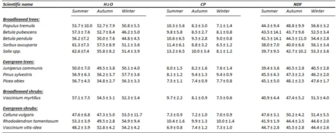
Table 2: Seasonal mean values (± standard deviation) of H2O, CP and NDF, for each species analysed
3.1 Seasonality of H
2O, CP and NDF
In this section, I have analysed all the values belonging to each species, excluding the difference in content (i.e. leaves and twigs). Thus, for each species the mean value was calculated as the average of both twigs and leaves values included together.
When looking at water content (Fig. 3), broadleaved tree was found to be the group with the highest values during summer. In this group, seasonality played an important rule. The mean summer values were higher than an
23
average of 11% (+/- 8%) from summer to winter. For broadleaved shrub (bilberry) the seasonal water variation was not statistically significant (t918= 1.930, p=0.13).
The water content present in evergreen tree species remained steady throughout the whole year, excluding the effect of seasonality on water content (t918= -0.743, p=0.73). A totally different pattern was found in the evergreen
shrub’s species, which did not show a significant change in water content moving from summer to autumn (t918=
1.216, p=0.44), but it was significantly higher in winter (t918= -3.504, p< 0.01).
Overall, during summer evergreen shrubs had lowest water content when compared to all the other groups (broadleaved shrubs t918= 4.979, p<0.01; broadleaved trees t918= 9.696, p<0.01; evergreen trees t918= -5.171,
p<0.01), while broadleaved trees had a significantly higher water content than both groups of evergreen plants (evergreen trees t918= 3.790, p<0.01; evergreen shrubs t918= 9.696, p<0.01). No difference was found between
the two groups of broadleaved species (t918= -1.020, p=0.74) and between broadleaved shrubs and evergreen trees
(t918= 1.263, p=0.58). In autumn the only significant difference found was a lower water value in evergreen
shrubs, when compared to all the other groups (broadleaved shrubs t918= 2.883, p<0.01; broadleaved trees t918=
3.109, p<0.01; evergreen trees t918= -3.091, p<0.01). Oppositely, during winter no differences were found in
between the groups, with the only exception for the broadleaved trees that had a significantly lower water content than all the other groups (broadleaved shrubs t918= 2.880, p<0.05; evergreen trees t918= -6488, p<0.01; evergreen
shrubs t918= -5.716, p<0.01).
Fig. 3: Seasonal change in water content in 4 different groups. The groups here listed are broadleaved shrubs (bilberry) and
trees (aspen, rowen, birches and Salix), evergreen trees (pine, spruce and juniper) and shrubs (lingonberry, header and Labrador tea).
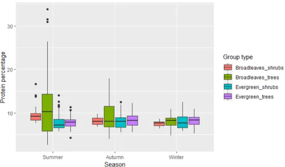
CP level was found to be significantly higher in broadleaved species (shrubs and trees) than the one measured in evergreen species (shrubs and trees) during summer (p<0.01). No difference was found between broadleaved shrubs and trees (z= 1.819, p=0.26), neither between evergreen shrubs and trees (z= 0.004, p=1.0). Nevertheless,
24
the difference in CP between groups disappeared in autumn and winter, where the level of CP was very similar, showing a non-significant difference between them (Fig. 4).
Overall the CP content showed a seasonal pattern in broadleaved species, to a greater degree in trees (z= -7.493, p<0.01) than the one recorded in the shrubs (z= -2.503, <0.05). In the evergreen species (shrubs and trees), proteins were not affected by the seasonality, remaining steady towards the whole year (z= 0.419, p=0.91 for evergreen shrubs and z= 1.179, p=0.47 for evergreen trees).
Fig. 4: Seasonal change in protein content in 4 different groups. The groups here shown are broadleaved shrubs(bilberry) and
trees (aspen, rowen, birches and Salix), evergreen trees (pine, spruce and juniper) and shrubs (lingonberry, header and Labrador tea).
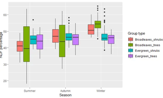
When looking at the seasonality effect on NDF value, fibre overall increased from summer to winter in broadleaved trees and shrubs (respectively t944= -14.657, p<0.01 and t944= -4.885, p<0.01). Nevertheless,
evergreen trees and shrubs were not affected by a seasonal change in NDF content (t944= - 1.179, p=0.46 and
t944= - 1.362, p=0.36 respectively). I found that in the summer evergreen shrubs had averagely higher NDF than
broadleaved trees (t944= -3.830, p<0.01), due to the big variation found in the broadleaves.
During autumn, the difference in NDF between groups was minimal, while a strong difference was found in the winter between broadleaved trees and evergreen species (t944= 8.886, p<0.01 for evergreen trees and t944= 5.827,
25
Fig. 5: Seasonal change in NDF content in 4 different groups. The groups here shown are broadleaved shrubs(bilberry) and trees
(aspen, rowen, birches and Salix), evergreen trees (pine, spruce and juniper) and shrubs (lingonberry, header and Labrador tea).
Finally, NDF content was found to be negatively correlated with crude protein (Multiple R-squared = 0.62, p ≤0.01) within broadleaved species across the season. The relationships showed on the left side of Fig. 6, explain that the CP level during summer is relatively high while NDF is relatively low for broadleaved species, and vice versa during winter.
The seasonal relationship between NDF and protein was not significant in the evergreen species (Multiple R-squared = 0.04, p=0.37) since it was not found a clear pattern between species belonging to this group.
Fig. 6: Linear relationship between NDF and CP in broadleaved (on the left side) and evergreen (on the right side) species. The
broadleaved plants (aspen=As, rowan=Ro, Salix=Sal, silver birch=SB, downy birch=DB, bilberry=Bb) showed a negative correlation between NDF and crude protein throughout the year (r =0.62, p ≤0.01). On the other hand, no
relationship (p=0.37) between the two nutritional components was found in evergreen species (heather=Cal, lingonberry=L, Labrador tea=Lt, juniper=J, pine=Pi, spruce=Sp).
26
3.2 Nutritional value in leaves, twigs, and twigs with leaves
For the analysis based on the different browsing options, leaves and twigs for broadleaved tree’s samples were analysed separately (see Chapter 2.4.), while broadleaved shrubs, evergreen shrubs and trees samples, twigs and leaves were processed together.
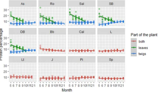
Overall, I found that the leaves of broadleaved species had the highest amount of CP than any other group with an average of 15.9% (+/- 4.9%), recorded in summer. In fact, this group contained a statistically higher amount of CP than twigs (of the same group) during summer (+9.8%) and autumn (+4.3%) (p<0.01 and p<0.01 respectively). CP recorded in leaves, were also found to be significantly higher if compared to the group so-called “both” (p<0.01), which consisted in twigs and leaves together (Fig. 7).
In the group “both” I did not find any seasonality trend, despite the higher protein content during summer (p<0.01) and autumn (p<0.01) than the twigs only.
Fig. 7: Monthly change in CP among the samples’ components in each species (aspen=As, rowan=Ro, Salix=Sal, silver
birch=SB, downy birch=DB, bilberry=Bb, heather=Cal, lingonberry=L, Labrador tea=Lt, juniper=J, pine=Pi and spruce=Sp). Plants were grouped based on the browser’s behaviour: both (i.e. include leaves and twigs for evergreen trees, shrubs and broadleaved shrubs), twigs and leaves (i.e. categories obtained by the separation of samples collected
from broadleaved trees).
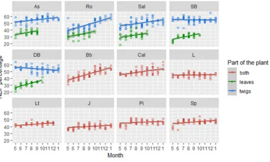
The analysis done on the NDF sample’s content established that leaves had an average 12% (+/-4.8%) lower NDF than the group “both”, containing leaves and twigs (p<0.01). Twigs on its own were the group with the highest NDF content (Fig. 8), having an average 7 % higher NDF than the samples containing both leaves and twigs (p<0.01).
A lower value of NDF was found in twigs during the vegetational season (i.e., summer and autumn), but once this season was over, it turned up to be significantly higher (p<0.01). For the samples with both twigs and leaves, I recorded a significantly lower NDF content during summer (p<0.01), which became higher in autumn.
27
Similarly, but to a major degree, seasonal change in NDF content was found also in leaves, which had lower values during summer if compared to autumn (p<0.01).
Fig. 8: Monthly change in NDF among the samples’ components in each species (aspen=As, rowan=Ro, Salix=Sal, silver
birch=SB, downy birch=DB, bilberry=Bb, heather=Cal, lingonberry=L, Labrador tea=Lt, juniper=J, pine=Pi and spruce=Sp). Plants were grouped based on the browser’s behaviour: both (i.e. include leaves and twigs for evergreen trees, shrubs and broadleaved shrubs), twigs and leaves (i.e. categories obtained by the separation of samples collected
from broadleaved trees).
3.3 Effect of latitude and habitat
Overall, the mean value of water content found in NM during summer (p<0.01) and autumn (p=0.05) to be significantly (and closely to be significant in autumn) higher than the one found in OM. The non-significant difference was found during winter (p=0.82) between the two areas.
When looking more closely at the latitude effect on water content, I found that the significant difference existing between NM and OM was restricted to the broadleaved trees species in the two areas (p <0.01), while for all the other groups the area did not affect water content.
Regarding CP, latitude was found to have statistically significant interaction with the season (p<0.01) and also with species (p<0.01). Based on the pairwise analysis run on the interaction between season and area, I revealed that the mean values of protein for each area were found to be close to significant difference only during winter (p=0.05), where OM had in average higher protein. Furthermore, when I looked at the species-area interaction, heather (p=0.01), lingonberry (p<0.01) and juniper (p<0.01) showed a strongly significant difference in mean values between the two areas, Salix (p=0.07) was close to being significant, whilst for all the other species was not recorded any statistically significant difference.
28
According to a three-way ANOVA, the latitude effect on NDF was overall not significant (p=0.53) for the species interaction, as well for the season interaction (p=0.44). However, a pairwise analysis was done for better understanding of the scenario. The mean values for NDF in NM and OM resulted to be slightly significant during summer (p<0.05) and autumn (p<0.05), where NDF was lower in NM in both cases. My results suggested no difference in NDF values between NM and OM , except of heather (p=0.05), bilberry (p=0.01) and downy birch (p<0.05) that higher NDF values in OM compared to NM.
According to my model, the interaction of protein measured in the 12 plant species and habitat type was not significant (p=0.25), likewise the interaction between season and habitat (p=0.98). The absence of a habitat effect is shown in Fig. 9 where all the habitat types seem to present a similar seasonal CP trend within each species. Similarly to what I saw for the CP, the model run on NDF demonstrated that the interaction between species and habitat, as well as the interaction between season and habitat, was not found to be statistically significant (p=0.99 and p=1.0 respectively) (Fig. 10). Note that for this specific analysis I have selected habitats which presented at least 3 measurements per species. All the habitat with less than 3 monthly measurements per species were excluded.
Fig. 9: Habitat effect on protein content, for all the 12 species sampled(aspen=As, rowan=Ro, Salix=Sal, silver birch=SB, downy
birch=DB, bilberry=Bb, heather=Cal, lingonberry=L, Labrador tea=Lt, juniper=J, pine=Pi and spruce=Sp). Habitat type here listed are clear-cut planted (CCp), coniferous mixed forest (CFm), coniferous pine forest (CFp), coniferous
29
Fig. 10: Habitat effect on NDF content, for all the 12 species sampled(aspen=As, rowan=Ro, Salix=Sal, silver birch=SB, downy
birch=DB, bilberry=Bb, heather=Cal, lingonberry=L, Labrador tea=Lt, juniper=J, pine=Pi and spruce=Sp). Habitat type here listed are clear-cut planted (CCp), coniferous mixed forest (CFm), coniferous pine forest (CFp), coniferous
spruce forest (CFs), deciduous forest (DF), edge (E), mire (M), mixed forest (MF) and road edge (R).
3.4 Twig size
Twigs of shrubs species had too small diameters, which made impossible the comparison of their nutritional content based on their average diameter. Hence, in this section I decided to analyse only twigs of trees species which presented a wide variation of diameter measurements, spacing from 0.1 to 4 mm.
30
Twig size did not affect CP and NDF content when all the species were analysed together. However, a different scenario showed up when I included species in the model. I observed that for aspen (r2 = 0.26, F = 20.19, p < 0.
001), silver birch (r2 = 0.16, F = 12.36, p < 0. 001) and downy birch (r2 = 0.20, F = 14.42, p < 0.001) the CP
content and the average diameter measured in the terminal section of twigs were positively related (Fig. 11). The relationship in rowan (p = 0.81), Salix (p = 0.20) pine (p = 0.34) and spruce (p = 0.74) was found to be non-significant, because the CP content remained stable with the increment of the terminal radial section of the twigs. Regarding NDF for most of the broadleaved species such aspen (r2 = 0.14, F = 9.83 , p < 0.05), rowan (r2 = 0.28, F =21.64, p < 0.001), Salix (r2 = 0.15, F = 12.89, p < 0.001) and silver birch (r2 = 0.06, F = 4.59, p < 0.05) the NDF level increased with the increase of diameter. Contrarily, pine (r2 = 0.29, F = 28.63, p < 0.001) decrease its NDF with the increase in diameter.
For downy birch (p = 0.18) and spruce (p = 0.46) the change in terminal radial section of the twigs did not affect significantly the protein content in twigs, which remained constant (Fig. 12).
31
My experiment produced five main key findings. Firstly, overall seasonality variation was recorded in all three nutritional components analysed; CP and water decreased from summer to winter, whereas NDF increased. Broadleaved species were more affected than evergreen species, showing a large variation in all values during the summer, which then decreased during winter. A different situation was found for evergreen, where the seasonal variation recorded was very small for some species (e.g. CP in pine and NDF in spruce) and non-existing for others (e.g. lingonberry, Labrador tea and juniper). Secondly, the seasonal NDF-CP ratio showed a negative correlation between the two nutrients only for broadleaf, while for evergreen species the seasonal NDF-CP ratio was not significant. Thirdly, most of the high protein content was primarily found in leaves of broadleaved species during the vegetative season. During winter, however, pine and Labrador tea showed higher values for CP than the ones found in broadleaved twigs. The fourth finding showed whether for some species the twig size affected the NDF and CP levels. Aspen, silver and downy birch increased their protein content with the increase of the diameter, while aspen, Salix, rowan and silver birch raised the NDF levels with the increase of the twigs’ diameter. Finally, the fifth result concerned the habitat and latitude effect. No significant effect of habitat onto NDF and CP was found, while latitude affected water content and CP but not NDF.
4.1 Seasonality and latitudinal effect on nutritional content
WATERThe main functions of water in the leaves are the transportation of nutrients and maintenance of a stable temperature under sunlight. As I hypothesized, when looking at the seasonal variation in water I found that water content was affected differently between groups. Broadleaved species were the group most affected by the seasonal variation for this element. In fact, from a morphological perspective broadleaved species have bigger leaf surfaces than evergreens, but leaves are thinner which increases transpiration and conducive to the collection of water (Villar et al., 2013). For these reasons, more water needs to be stored in their leaves which explains why I found higher water percentage in broadleaves. Contrarily, evergreen species have leaves covered in wax and posses with pit-like stomata, which prevent transpiration and improve water retention (Matyssek, 1986). Therefore, the effect of seasonality was not significant for evergreen species.
32
A different result was the higher amount of water content found in shrubs during winter when compared to their values recorded in summer and autumn. However, I believe that this finding can be explained due to the frozen layer of water condensation which is formed during the night and persist through the winter days.
Water content was different between the two study areas (i.e. NM and OM). To be able to understand the latitude’s effect on water content, I had to analyse meteorological data collected during the whole length of the study from the weather stations nearby the two study areas (Florida A for OM and Järnäsklubb for NM). As shown in Appendix 4, monthly rainfall and monthly average air temperature were non-significant (p = 0.95 and p = 0.51 respectively), however, relative humidity it was significantly higher in NM (p < 0.05). It has been shown that higher relative humidity (as well as rainfall) could decrease the evaporative demand which implies higher water retention in plant tissues (Bradley et al., 1987). This may explain why species in NM showed on average higher water percentages than in OM. However, to better support this conclusion I should have also measured the water content in the soil which highly influences the water content in plants (Ritchie, 1998). This should be considered in future studies.
PROTEIN
Similarly to what I found for water content, overall CP too was affected by the seasons. Interestingly, evergreen species did not show any significant seasonal change in the protein, whereas broadleaved species had a consistent change between seasons. This result did not confirm my second hypothesis (i.e. wehther seasonal variation in CP should be consistent in all species).
Nitrogen content in the leaves is represented by the proteins produced during photosynthesis (Evans, 1989). Thus, the amount of nitrogen is approximately proportional to the chlorophyll content. Because broadleaved species shred their leaves, preceded by a gradual reduction in chlorophyll levels across the seasons, CP content in the leaves can also be expected to decline throughout the year. On the other hand, it has been found that nutrient remobilization (i.e., nitrogen and phosphorus) in evergreen species is mainly driven by the growing demand (Milla et al., 2005). I therefore were expecting to see a seasonal variation in CP, consistent for all the species. However, according to what I found, remobilization of nutrients (as the redistribution of N) seems to occur mainly in branches (Nambiar and Fife, 1991), and usually when the environmental availability of nutrient in the soil is low as well as during the growth of new organs (Millard, 1994). In addition, some evergreen plants (e.g., pine) do not seem to be capable of withdrawing N from deposits in their needles. For this reason, evergreen species keep the overall level of CP steady in the terminal shoots (which are subject to most of the browsing impact), and thereby ‘hiding’ the seasonal variation of CP in the plant. Even though I have not found any significant difference in CP between groups, when looking at species resolution, nitrogen content per unit dry weight was highest in Salix during summer, while Labrador tea followed by pine had the highest amount of CP in winter (Table 2). This could explain why conifers are usually preferred by browsers in winter while broadleaf species are favoured during summer (Gill, 1992). Furthermore, bilberry was found to have a higher protein content during summer and autumn than the other two species (lingonberry and heather) which belonged to the same family of
33
Ericaceae; this could explain their importance as staple food item for ungulates. Within evergreen trees species, the CP in pine was found to be significantly higher than Juniper and spruce during winter. The comparison between downy birch and silver birch did not show any significant difference in CP throughout the year. According to my results, latitude affected CP. Heather, lingonberry and juniper were found to have lower CP in NM than in OM. Unfortunately, with the information collected, I was not able to find an explanation for this result. During the fieldwork in OM I realized that the availability and the height of shrubs were much lower in this area when compared to NM further north. Furthermore, the composition and abundance of the ungulate community differ between the two sites. In the north, Cervid densities tend to be lower with the main species being moose, roe and red deer, whereas in the southern area the density of ungulates is much higher, largely due to high numbers of fallow deer and red deer. Thus, the presumably higher foraging pressure on the forest field layer might affect the growth of ericaceous shrubs such as lingonberry and heather, leading, perhaps, to foliage containing more chlorophyll (and as consequence CP). A similar scenario was recorded by Moe et al. (2018) in browsed bilberry. However, more studies are needed to investigate this question.
NDF
Looking through the literature available on NDF, it is generally reported as a rough estimator of animal’s intake of DM (i.e. as NDF increase DM intake will decrease) and the time of rumination (González-Hernández and Silva-Pando, 1999). I must not forget that cellulose and hemicellulose are the main fuel for ruminants, typically providing up to 80% of their energy (Barboza et al., 2008). So, at higher levels of NDF, the richer the DM in fibre will be, and lower DM will be needed to satisfy requirements. On the other hand, I need to keep in mind that NDF alone does not give us any information related to fibre quality (Vogel et al., 1999). In fact, NDF content includes lignin which is essentially an indigestible compound (Jung et al., 1997). It has been shown that usually when fibre content increases, digestibility decreases but the concentration of secondary metabolites that possibly inhibit digestibility may also decrease (Palo et al., 1992). Therefore, I have used these guidelines to base my interpretation for the NDF analysis’ outcome.
Overall, NDF showed an opposite trend to the one recorded for CP and water, with a general increase of NDF concentration per unit of DM moving from summer to winter. Once again, the change in seasons strongly affected broadleaf species, but not evergreen species that retained constant levels of NDF throughout the year. The seasonal transition recorded, showed that during summer broadleaves had a much lower NDF than evergreens, but the difference between groups then became marginal during autumn. In winter, however, the broadleaves showed a higher NDF than evergreen. According to Chapin (1980) evergreen species have a particular strategy to maintain the foliage, which consists of reducing the seasonal investment in carbon and other nutrients. On the contrary, it has been recorded that leaf development through the growing season in broadleaves, show an increase in the lamina thickness, tissues maturity and photosynthesis efficiency (Dickson, 1989). This explains why seasonality does not affect evergreens as much as the broadleaf plants.
34
For the NDF values, the latitude effect was not significant. Davi et al. (2006) demonstrated that high temperatures can increase autotrophic and heterotrophic respiration, decreasing as a consequence the gross primary production, within the same species. Therefore, I would expect a decrease in NDF values if the average temperature had been higher in OM. In this case, even though the average seasonal air temperature was slightly higher in OM, the overall statistical analysis did not reveal a significant difference in temperature between the two areas.
NDF‐CP Ratio
As reported by Tamminga et al. (1990),the NDF-CP ratio can vary widely between different forage species, also in my study a non-clear relationship was recorded when all the species were analysed together. Despite this, when plant’ groups were inspected separately, the ratio between NDF and CP was highly significant and explained 47% of the seasonal variation between the two nutrients.
The relationship found in broadleaves was mainly linked to the strong but opposite seasonal trend of CP and NDF, that was similarly followed by all the species belonging to this group; in this group the NDF-CP ratio explained the 62% of the seasonal variation. This principle can be applied also for the evergreen species. In fact, the ratio was non-significant which may have been due to an inconsistent seasonal pattern in NDF and CP within the species belonging to the same plant’ group.
4.2 Browsing options and their nutritional values
As I mentioned in the previous chapter, chlorophyll and CP are proportionally related. This led us to the hypothesis that CP should be found with higher concentration in leaves compared to twigs during the vegetative season. In fact, according to the analysis’ results on the browsing options (i.e. twigs, leaves, and twigs and leaves together), I found that the leaves had much higher CP content than any other browsing option. Contrarily, leaves of broadleaf species had a much lower NDF content than the twigs and twigs and leaves together. Twigs, however, were found to contain the highest amount of NDF but lowest levels of CP throughout the whole year. A similar result was reported by the Council (2007) showing that the buds and leaves are usually higher in protein and lower in lignin content, acid detergent fibre (ADF) and tannins than twigs.
Opposite to what I had hypothesized, based on the result of twigs radial section and their nutrient content, I was able to detect a clear pattern only in evergreen trees (i.e., pine and spruce). In both species, CP remained steady with the increase of the average diameter. An analogous result was found for NDF in spruce, but pine twigs with larger diameter showed slightly lower values for NDF. Oppositely, one study done on pine between the relationship of twig diameter and nutrients was found, showing that NDF content increased with increasing twig diameter, while CP decreases (Jia et al., 1995).
A different scenario was found for broadleaf trees. In fact, apart from downy birch, the broadleaved species increased their NDF content with the increase of twig’s diameter. However, for protein, only aspen, silver and downy birch increased CP with increasing in diameter, while rowan and Salix remained stable. Studies done on