Congestion Management at the Network Edge

M¨

alardalens H¨

ogskola

Thesis for the Degree of Bachelor of Science

in Engineering

Computer Network Engineering

Congestion Management at the

Network Edge

Author:

Oscar Daneryd

Supervisor:

Conny Collander

Examiner:

Mats Bj¨

orkman

September 17, 2014

Contents

6.3 Quality of Service vs Quality of Experience . . . 15

6.4 No knobs . . . 15

7 Method 16 7.1 Tail Drop . . . 16

7.2 Random Early Detection (RED) . . . 16

7.3 CoDel . . . 18

7.4 FQ CoDel . . . 18

7.5 PIE . . . 19

8 Solution 21 8.1 CeroWRT . . . 21

8.1.1 Installation and Configuration . . . 22

8.3 Testing Hardware . . . 23

8.4 Testing Procedure . . . 24

9 Results 28 9.1 Web Browsing With Delay . . . 28

9.2 Real-Time Response Under Load . . . 30

9.2.1 Taildrop . . . 31 9.2.2 CoDel . . . 32 9.2.3 FQ CoDel . . . 33 9.2.4 PIE . . . 34 9.2.5 ARED . . . 35 9.2.6 SFQ . . . 36 9.2.7 Comparison . . . 37 9.2.8 ECN . . . 39 9.3 Recommendations . . . 39

9.4 Problems during testing . . . 39

9.4.1 Further Work . . . 40

10 Conclusion 41

11 Summary 42

1

Abstract

In the Internet of today there is a demand for both high bandwidth and low delays. Bandwidth-heavy applications such as large downloads or video streaming compete with more delay-sensitive applications; web-browsing, VoIP and video games. These applications represent a growing share of Internet traffic.

Buffers are an essential part of network equipment. They prevent packet loss and help maintain hight throughput. As bandwidths have increased so have the buffer sizes. In some cases way to much. This, and the fact that Active Queue Management (AQM) is seldom implemented, has given rise to a phenomenon called Bufferbloat.

Bufferbloat is manifested at the bottleneck of the network path by large flows creating standing queues that choke out smaller, and usually delay-sensitive, flows. Since the bottleneck is often located at the consumer edge, this is where the focus of this thesis lies.

This work evaluates three different AQM solutions that lower delays without requiring complicated configuration; CoDel, FQ CoDel and PIE. FQ CoDel had the best performance in the tests, with the lowest consistent delays and high throughput. This thesis recommends that AQM is implemented at the network edge, preferably FQ CoDel.

1.1

Abstract in Swedish

I dagens Internet finns det ett behov av b˚ade h¨og bandbredd och l˚aga f¨ordr¨ojningar. Applikationer som anv¨ander mycket bandbredd, t.ex. videostr¨omning, m˚aste dela n¨atet med f¨ordr¨ojningsk¨ansliga applikationer. Exempel p˚a dessa ¨ar websurfande och datorspel. Dessa applikationer representerar en v¨axande del an Internettraffiken. Buffers ¨ar en viktig komponent i n¨atverksutrustning. De motverkar paketf¨orluster och m¨ojligg¨or en h¨og genomstr¨omning. H¨ogre bandbredder har lett till st¨orre buf-frar. I vissa fall oproportionerligt stora bufbuf-frar. Detta i kombination med att Aktiv K¨ohantering (AQM) s¨allan implementeras ger upphov till fenomenet Bufferbloat. Bufferbloat uppenbarar sig i flaskhalsen p˚a en l¨ank genom att stora fl¨oden av trafik skapar st˚aende k¨oer som stryper trafiken fr˚an mindre, oftast f¨ordr¨ojningsk¨ansliga, fl¨oden. Fokus ligger p˚a konsumentn¨at d˚a de oftast inneh˚aller flaskhalsen.

Denna uppsats har utv¨arderat tre AQM-l¨osningar som s¨anker f¨ordr¨ojningar utan komplicerad konfiguration; CoDel, FQ CoDel och PIE. FQ CoDel presterade b¨ast i de utf¨orda testerna, med l˚aga f¨ordr¨ojningar och h¨og genomstr¨omning. Denna uppsats rekommenderar att AQM implementeras i konsumentn¨at, f¨orslagsvis med FQ CoDel.

2

Purpose

The purpose of this thesis is to explore the problem of Bufferbloat in relation to consumer and small business networks. A few of the proposed solutions to this problem will be evaluated as well as their applicability. The main technical solution that will be examined is the use of AQM and how this affects the experience of the network user.

Due to the time allotted, the work will be focused on queue management at the network edge. There is more to Bufferbloat than just the lack of AQM, unmanaged buffers and queues can be located anywhere. They can hide in the application itself, in the protocol and device drivers, even in the networking hardware. This is beyond the scope of this thesis. The delay inside the Internet itself, caused by things like over-subscription, peering issues and physical limitations, like the speed of light, is also outside the scope of this thesis. Even thought a lot of the problems and perhaps even the solutions are relevant to the Internet at large, the main focus lies inside the network edge.

The feasibility of implementing the solutions will be explored to determine if it could be done for (or by) the average user. This is an important part since configuring network equipment can be difficult and most users would prefer not having to do it at all. This is a current topic but not very well known. Therefore the purpose of this thesis is also to inform and educate people on the subject, especially those interested in networking.

3

Background

When considering topics for my thesis I was at the onset interested in latencies. I had just finished reading the book ”Flash Boys” by Michael Lewis about High-Frequency Trading (HFT). In HFT you are not only concerned with milliseconds, even microseconds can make or break a trade. When a company is willing to spend 100s of millions of US dollars to lay a slightly straighter fiber optic cable between Chicago and New York just to shave off a few milliseconds you realize just how important low delays can be. While it is a very interesting subject, I realized that access to both hardware and software would be very limited. It also wasn’t really close to anything I had worked with before, making me unsure of where to start.

Moving up from nanosecond switching at Layer 1 and 2 I arrived at Quality of Service (QoS) which was a more familiar topic. In the course ”Optimizing Converged Networks”, and in other courses as well, I had studied and applied the concepts of QoS. Reading about the need for QoS I stumbled upon the problems associated with Bufferbloat and its prevalence on the Internet. Especially in consumer equipment. I had never considered this problem before. While WRED with DSCP markings from well behaved applications and automatic classifications would work in a large internal corporate network, something I had studied and knew about, I had never considered what the situation would be for a regular consumer or at a small business. Since this was a relatively new topic (especially the proposed solutions) it caught my interest. And since it also affects me personally, and everyone else that use the Internet, it became even more interesting.

4

Relevant Work

While the topic was not completely new[1][2], it had recently gained more widespread attention and several proposals on how to deal with it was being put forward and worked on. Jim Gettys, known for his work on the X Window System and the HTTP1.1 specification, popularized the term Bufferbloat and is working on raising awareness of the issue[3][4]. The Bufferbloat project was started in order to consolidate the efforts put into finding and exploring solutions to Bufferbloat[5]. Also included in the Bufferbloat project is the work on the AQM techniques CoDel and FQ CoDel and the routing-platform CeroWRT.

Part of the concepts behind CoDel was first envisioned in a unpublished paper by Kathleen Nichols and Van Jacobson, both well known in the Internet community, called ”RED in a different Light”[6] where another AQM technique called Random Early Detection (RED) was modified to be completely self-tuning. A couple of years later CoDel was proposed by the same duo[7]. Both CoDel and FQ CoDel have been defined in IETF RFC drafts[8][9] for standardization. Implementations of them have also been included in the Linux kernel. Both as a result of work done by Eric Dumazet at Google.

Inspired by the concepts behind CoDel, Cisco has proposed a modification to the PI algorithm called Proportional Integral controller Enhanced (PIE)[10] which has also been defined in an IETF RFC draft[11].

CeroWRT is a Linux routing platform based on OpenWRT that is used as a testing platform for the research done on Bufferbloat. CeroWRT is maintained by David T¨aht who also worked on the Linux implementation of CoDel and FQ CoDel and is an active proponent of its use as a solution to Bufferbloat.

There have been several papers published and presentations held at conferences on the topic of Bufferbloat where proposed solutions have been evaluated and tested[12][13][14]. Both CoDel and PIE, but especially FQ CoDel, have been shown to dramatically reduce Bufferbloat, resulting in low latencies and high link utilization. There is also active discussions on the dedicated Bufferbloat and IETF AQM mailing lists on the topic.

5

Problem Formulation

The Internet of today is very different from a couple of decades ago and so are the applications using it. With an increase in availability, reliability and speed of access, the content on the Internet has changed. App stores and the delivery of video and music through downloads and streaming is increasingly replacing physical media, putting demand on the download speed of the connection. More and more services are also provided in ”The Cloud” such as backup services for personal files and online photo and video libraries. For social media sites, user created (and uploaded) content such as audio, video and pictures is integral to their business model. All of these services utilize the users upload speed. Higher speeds arguably provide a better user experience.

But there is another category of applications that does not dependent on a high download and upload speed in the same way. These applications generally send small and few packets that instead need quick delivery and a low probability of failure. These are called interactive applications. This category instead relies on the latency of the connection. In other words, the length of the delay between when an action is taken, and the expected response is presented, determines the quality of the user experience. These applications include things like voice and video chat, video games, but also the web and the technologies driving it.

While a web page might take a long time to load because its big, it could also be because the DNS packets that translate the domain names used on the page and the HTTP packets that request and deliver the content spend a long time in transit, even though they are small. This is caused by a long Round Trip Time (RTT). The RTT is the time it takes for a packet to travel from its source to its destination, and then back to the source again. A voice call over a link with a long RTT would experience delays in the delivery of the sound, possibly leading to users accidentally talking over each other. Voice calls are also susceptible to jitter, a high variance in RTT, leading to distorted or dropped sound. The same principles also applies to video chat. In online video games or in other interactive applications where commands from the keyboard, mouse and other input methods needs to be sent over the Internet, a large delay can be very frustrating for the user.

6

Analysis

Unfortunately bandwidth-intensive applications are very likely to cause delays for interactive ones. Since both types of applications are important to users, a perfect solution would have to provide for both without compromises.

The following sections describe in detail the technologies that affect the delays in the network.

6.1

Hardware

Buffers are an essential part of networking equipment. They allow for bursts of inbound traffic that exceed the outbound capacity of the link. These bursts include the transient bursts of conversation startup and the statistical multiplexing of traffic from different sources. The packets are enqueued in the buffer, and are dequeued on a first in first out (FIFO) basis as the outgoing link allows. When the buffer is full, all new incoming packets are dropped until there is room for more packets. Having a buffer ensures that the bottleneck link is maximally utilized during these conditions and tries to minimize packet loss. Since there can only be one slowest link in a path, as seen by a flow, there is only one bottleneck.

To ensure that the links can handle these bursts, the size of the buffers need to be adequate. These short-lived bursts generally disperse in one round trip time (RTT) so a good size would need to be at least the Bandwidth-Delay-Product (BDP): BW ∗ RT T = BDP . The BDP represents the maximum amount of data that can be in flight between endpoints. Since the RTT can vary between flows, as can the the bandwidth for some technologies, such as WiFi, the optimal buffer size can be hard to determine. Thanks to Moore’s Law, computer memory have both increased in capacity and decreased in price so that as bandwidths has increased, buffer sizes have increased. Also to accommodate so called Long Fat Networks (LFN), links with a very high BDP such as trans-continental fiber or satellite links,

and with the idea that packet loss is always bad, companies chose to err on the side of caution when setting buffer sizes.

But this is also prevalent in consumer and general network equipment. As previously mentioned, the availability of cheap memory gives manufacturers the opportunity to create products that can deliver huge bursts of traffic and perform

great in select benchmarks with high utilization and close to zero packet loss. But if these buffers are left unmanaged, performance, using delay as a metric, will suffer.

Protocols have different ways of trying to utilize as much as possible of the available resources. The Transmission Control Protocol (TCP) has a built in congestion control and tries to match its windows to the BDP while applications using the User Datagram Protocol (UDP) has to try to adjust its send rate on its own. This presents a problem as the bottleneck is (usually) somewhere in the network and the send rate is determined by the endpoints. Because of factors such as changing link rates as determined by Layer 1 and 2 protocols or redirection of traffic, the size of the bottleneck might change during transmission. This mismatch in the perception of the BDP can lead to the endpoints putting too much data in flight. If the receiver in a TCP conversation advertises a window that is bigger than the BDP, for example a long-lived connection with a 30 packet window for a 20 packet BDP, the extra packets sent does not affect the throughput and the 10 extra packets in this example will create a constant standing queue at the bottleneck with those 10 packets only creating delay[7].

This standing queue combined with the huge unmanaged buffers is Bufferbloat.

6.2

Software

UDP is a transport layer datagram protocol. It provides a minimum of protocol features and is therefore simple and provides low overhead. It is unreliable in that it cannot guarantee packet delivery, or even an indication that the delivery was successful. It provides no congestion control or ordering of packets, leaving these tasks to the application layer. Since it provides low overhead it is often used for time-sensitive applications such as VoIP. A missing packet in a VoIP conversation might not even be useful any more if it were to be resent, making such features superfluous.

Even though UDP does not have build-in congestion control it is highly recom-mended it is implemented in the application using it. This is so it does not choke the flows of other protocols and gain an unfair advantage in packet delivery[15]. TCP is a transport layer protocol that is part of the IP suite. It is the most used used transport protocol on the Internet. TCP provides ordered and reliable

delivery, error checking and congestion control. To limit the scope of this thesis, only topics relating to the congestion management of TCP will be studied.

TCP uses two windows to manage the amount of data sent onto the network. The receive window (rwnd ) is an indication of how much data the receiver in a TCP conversation can receive and process. This amount is defined by the Window Scale Option as a value between 64KB and 1GB.[16] The second window is the congestion window (cwnd ). The cwnd regulates how much data the the sender can send before receiving an ACK. The smallest value of rwnd and cwnd ultimately decides the window size used, i.e. how much data that can be sent.

There are four algorithms that governs the size of the cwnd.

Window Size

ssthresh1

ssthresh2 ssthresh3

Time

Triple Duplicate ACK RTO Timeout

Slow Start

Congestion Avoidance

Fast Retransmit

Fast Recovery

Figure 1: The standard TCP algorithms

6.2.1 Slow Start

Slow start is first used to increase the cwnd after a completed three-way handshake. The initial window (IW) is set to a maximum of IW = 4 ∗ SM SS depending on Sender Maximum Segment Size (SMSS) and is increased by one SMSS for

each received ACK. This essentially leads to exponential growth of the window (delayed ACKs will slow down the rate). Unless a loss is detected during Slow Start, the window continues to grow until it reaches a set threshold (ssthresh) where congestion avoidance takes over. If a loss is detected the Slow Start process starts over[17].

6.2.2 Congestion Avoidance

During congestion avoidance, the sender in not allowed to increase the cwnd by more than SMSS every RTT. A common formula for this is

cwnd += SM SS ∗ SM SS cwnd

which leads to a linear increase of cwnd. If a loss is detected the value of ssthresh is reduced according to

ssthresh = max(F lightSize

2 , 2 ∗ SM SS)

where FlightSize is the amount of data currently traveling between the endpoints. This effectively halves the ssthresh and sends cwnd back into Slow Start with a starting size of SMSS[17].

6.2.3 Fast Retransmit

When an out-of-order segment arrives the receiver immediately transmit a duplicate ACK indicating the expected sequence number. When the sender receives 3 duplicate ACKs, it assumes a segment has been lost and immediately resends lost data without waiting for the Retransmission Timeout (RTO) to expire (the RTO is calculated based on the Round Trip Time (RTT) but is always rounded up if <1 second). The logic is that since the 3 duplicate ACKs must have been generated by later packets that actually arrived, the congestion is over and it is safe to resend[17].

6.2.4 Fast Recovery

Since a loss occurred, cwnd would have to be reset and start over with Slow Start. Instead Fast Recovery takes over. ssthresh is set to

ssthresh = max(F lightSize

and after the lost segment is retransmitted, cwnd is set to cwnd = ssthresh + 3 ∗ SM SS

(the three segments that the receiver already has since it sent the duplicate ACKs for them) and is increased by SMSS for each additional duplicate ACK. During this time new unsent data can be sent if cwnd and rwnd allow it. When the lost segment is acknowledged, cwnd is set to ssthresh and congestion avoidance begins[17].

6.2.5 Other TCP improvements

There are several other improvements that has been made to TCP that might indirectly affect the cwnd.

Round-Trip Time Measurement The RTT for a packet used to be calculated using a sample taken once every window. Since this can lead to inaccurate measurements, especially for large windows, the TCP Timestamp Option was proposed. A timestamp is placed in each segment that is then replied back in an ACK. Simply subtracting the replied value from the current time gives the RTT[16].

Selective Acknowledgement (SACK) To help the Fast Retransmit/Recovery algorithms deal with multiple losses in a window worth of time, SACKs are used. If a segment is lost or an out-of-order segment arrives, this option notifies the sender of which segments (up to 3) were last received. This informs the sender of the segments that the receiver currently have in its receive queue so that it can resend the missing segments[18].

Protect Against Wrapped Sequence Numbers (PAWS) The TCP

se-quence number is a 32bit value. If this number were to wrap around during a TCP conversation it could falsely indicate duplicate segments. If it were to arrive within the current window it could supply the application with the wrong data since the checksum would still be correct. This it not a problem at slow speeds but at 1Gbit speeds it would wrap around in 17 seconds and at 10Gbit in 1,7 which is

well within the time a segment might spend in a queue. To solve this the PAWS algorithm is used. PAWS looks at the timestamp option in the TCP header and if the vale is less than the value of a segment that was recently received, it can be discarded[16].

Explicit Congestion Notification (ECN) Packet drops works as a natural indication of congestion since the router might simply not have enough resources to do anything but ignoring, and thus dropping, the packet. But packets are sent for a reason and unnecessary packet loss should be avoided. An alternative to packet drops is to mark the packet to indicate congestion. When AQM is used, packets are dropped before the router is completely congested so handling the packet is still possible.

In IP and TCP this is done using the ECN header in the IP packet. The last two bits of the old ToS octet in the IP header is used to indicate if it is an ECN-Capable Transport (ECT) and if it has had a Congestion Experience (CE) in the path. When a router in the path start sensing a congestion coming on and decides to drop a packet, it first looks at the IP header of the packet to see if it has the ECT flag set. If it does the router has the option to, instead of dropping the packet, send it as usual but with the CE flag set.

When a packet arrives at a host with CE set in the IP header, the receiver sets the ECN-Echo (ECE) flag in the TCP header of its returning ACK-packet. A host that receives an ECE packet reacts as it would for a dropped packet (except of course resending the packet) and send a reply with the Congestion Window Reduce (CWR) flag set in the next TCP segment[19].

6.3

Quality of Service vs Quality of Experience

When talking about Quality of Service (QoS) in reference to networks, the general concept concerns a series of quantifiable values that can be measured and compared to a set of requirements. QoS is affected by things like throughput, delay, jitter, errors and the order of delivery, and QoS is used to make sure the values of these variables are at an acceptable level. This is usually done with different types of reservations of resources for the desired traffic. But for most users these values do not mean anything, and they certainly would not want to configure them. The average Internet user would not call up his ISP and complain about out-of-order packet delivery, high RTTs or unacceptable levels of jitter. Either the Internet is fast or slow.

A better name for the end-users subjective perception of how well the network works is Quality of Experience. This would also include the users ability to use their applications in a satisfactory way and the amount of configuration needed to do so.

6.4

No knobs

The technical knowledge required to configure a router is a something most people have neither time nor interest to acquire. Manually tuning TV-stations with a knob or having to program whatever application you might need for your computer in BASIC is a thing of the past. And a small business would probably prefer to keep IT related costs and issues at a minimum.

Therefore, pretty much everything you can buy in terms of consumer electronics is nowadays Plug and Play, some even contain no instruction manual beyond a sheet of paper showing you how to turn it on. This includes home routers. Even some enterprise equipment can hold your hand through a short configuration that is essentially set and forget. A home router that you buy today will provide every client with an IP address through DHCP, have its default SSID-name and Pre-Shared Key printed on the back and this is all most users usually need.

A technical solution to the aforementioned problems would then have to be without configuration requirements, invisible to the user and work in a wide variety of network configurations and with varying traffic patterns without having a negative effect on performance.

7

Method

7.1

Tail Drop

Tail Drop is the most basic form of queue management and is the default in most equipment. It never drops packets until the queue is full, and then the device simply drops all new incoming packets until it has space available in the queue again. It does this indiscriminately from all flows and no matter the packet. A consequence of this is that since a lot of packets are dropped, TCP backs off and reduce its send rate.

If packets from many different TCP flows are dropped at essentially the same time, they slow down their send rate at the same time, producing an oscillating traffic pattern leading to low bandwidth utilization. This phenomenon is called global synchronization.

7.2

Random Early Detection (RED)

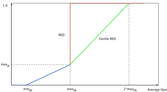
RED uses random dropping of packets before it is enqueued in order to control the queue size[20]. A consequence of the drops being random is that the probability of a drop is proportional to the bandwidth a flow uses. RED measures the average queue length to get a picture of the congestion. An instantaneous measurement of the full queue size would not take bursty traffic that only temporarily fills the buffer into account and thus makes unnecessary drops affecting throughput.

The packet dropping probability is calculated using the formula

p = pb

1 − packets since last dropped packet ∗ pb where

pb = max probability(average queue size − min threshold) max threshold − min threshold

and

average queue size = (1−queue weight)∗previous average+queue weight∗queue length The variables in these equations are set to user-configurable values. The original

max threshold set to at least twice the size of min threshold and queue weight = 0.002.

When the average queue size surpasses the minimum threshold, RED starts dropping packets and keeps dropping with increased probability until the maximum threshold is reached at which point all new packets are dropped. A modification to RED has been made called ”Gentle RED” that linearly increases the drop probabil-ity from max probabilprobabil-ity up to 1.0 between max threshold and 2 ∗ max threshold to prevent the instant jump to full dropping mode.

The values of the thresholds need to be configured based on available queuing space, bandwidth and typical RTT. The queue weight needs to be lowered in high speed networks so that the average queue length is updated more often and the maximum drop probability have several different recommended values. To reduce the configuration requirements, another modification has been made called Adaptive RED (ARED)[21] that dynamically tunes these values to try and reach a target average queue size. This target queue size still needs to be manually configured.

Drop Probability

Average Queue maxp

minth maxth 2*maxth

RED

Gentle RED 1.0

7.3

CoDel

The usage of queue length as a metric of congestion is problematic. The length depends of how and when you measure it. If you for example use the average length on a well-behaved burst of traffic that disperses in one RTT, it would falsely indicate a standing queue with a length of just under half the burst size. It also provides an inaccurate picture of the congestion if it is measured on a link with varying speed, such as WiFi.

The idea behind CoDel is to try to control the delay itself that is caused by the queue. This delay can easily be measured by giving each packet a time-stamp when it is enqueued and comparing it to the time it is dequeued. This sojourn time is measured during an interval based on the maximum experienced RTT (starting at 100ms). The goal is to control the minimum delay (5% of the RTT) in this interval. The minimum delay is used to separate a bad queue from a good queue. A good queue is a queue that will disperse during one RTT. A minimum delay of 0 would indicate that there is no standing, or bad, queue.

When the delay is consistently above the set minimum delay during the interval, packets are dropped at the head of the queue. If any packet in the interval is below the minimum delay, the timer is reset. Packets are dropped with increasing frequency if the delay remains or increases. The delay between drops is calculated using 1/√x where x is the number of drops since dropping started. CoDel does not drop packets if doing so would leave the queue with less than one MTUs worth of packets since this could have a negative effect on the throughput.

7.4

FQ CoDel

Instead of using one queue for all flows in a buffer, FQ CoDel tries to give each flow its own queue. The flows are separated by hashing a 5-tuple value from the packet (default is src/dest port/ip and protocol) together with a random number. Because of hash collisions flows might end up in the same queue, but the probability is generally low. These principles are similar to those used in Stochastic Fair Queuing (SFQ). Each separate queue is then controlled by its own instance of CoDel in

much the same way as CoDel works on its own.

1024 queues are created by default and they are served in a Round Robin (RR) fashion by a scheduler based on Deficit Round Robin (DRR). The scheduler

separates the queues into new and old. New queues are queues that do not build up a standing queue, i.e. they are empty within one iteration of the scheduler while old queues still have data in them. Each queue starts out with a quantum, a byte deficit of 1514 bytes (MTU of Ethernet plus the 14 byte header). During every round of the scheduler, the CoDel algorithm is run on the queue and it is allowed to dequeue at least quantum bytes worth of packets. It continues until the deficit reaches a negative at which point quantum bytes is added to the deficit and the scheduler continues on to the next queue.

Each of the new queues are either emptied or have their quantum worth of packets dequeued after which they are moved to the list of old queues. The scheduler then moves on to the list of old queues and does the same thing. If an old queue is emptied it is removed entirely and is not added again until a new packet that matches its hash arrives, at which point it is added back as a new queue.

7.5

PIE

PIE is an algorithm similar to CoDel proposed by Cisco. PIE is based on the PI algorithm[22] but has been reworked to use queuing latency instead of queue length as a metric of congestion. PIE does not need to use timestamps or any type of packet manipulation and since it drops packets before it is enqueued, PIE uses less memory and resources than CoDel which may simplify its implementation in some hardware.

Like the RED algorithm, PIE calculates a drop probability to determine if a newly received packet should be randomly dropped or enqueued. The drop probability p is calculated using

p = p + α ∗ (current delay − ref erence delay) + β ∗ (current delay − old delay) every update interval.

α and β are set to a value between 0 and 2 where a typical value for α would be 0,125 and 1,25 for β. The α part of the function is influenced by the deviation from the reference delay while the β part indicates whether the delay is increasing or decreasing. In order to maintain stability and have the ability to respond to fast changes, the algorithm tunes the values of α and β according to the previous value of p. If the drop probability is low, so are the values of α and β. As p grows past certain set thresholds (1% and 10%), α and β are increased.

The value of the current queue delay is calculated using Little’s Law[23]: current delay = queue length

average departure rate

The reference delay is set to 20ms by default in the Linux implementation which is the delay the algorithm strives to achieve.

8

Solution

There have been several papers published evaluating the effectiveness of the previously mentioned queuing disciplines. A lot of them using the ns-2 Network Simulator or full sized desktop computers as routers. These tests serve well to provide a controlled environment in which to conduct comparative testing, but might not provide an accurate image of reality. The physical characteristics of technologies as well as slightly non-standard implementations can be hard to simulate. So to provide a real-world scenario it was decided to conduct the testing on a residential DSL-connection using a consumer router. This is not an as controlled environment as a lab or simulation but effort has been made to make the tests and results reproducible.

8.1

CeroWRT

OpenWrt is an open source routing platform for embedded devices. It is Linux-based and optimized for small size. It supports a wide range of hardware and has a large library of software supported by an active community.

Thanks to its wide support of hardware and software, OpenWRT has provided a platform for several other projects. CeroWRT is one of them. CeroWRT was started by the Bufferbloat project to serve as a testing platform for experimentation and evaluation of proposed Bufferbloat solutions. It comes pre-installed with software, patches and scripts to deal with Bufferbloat as well as a web-based GUI for configuration.

CeroWRT has pre-compiled builds for a few platforms from Netgear. The router used was the WNDRMACv2 which is a combined 802.11n wireless access point and 5-port gigabit router. It has a 16MB flash memory and 128MB of RAM.

8.1.1 Installation and Configuration

To install a custom firmware one can either use the web-based GUI to upload the file or use TFTP. Here TFTP was used. The router is started with the power button while holding down the reset button on the bottom until the power LED starts flashing green. This starts a TFTP-server that will accept a valid firmware file and write it to flash. No major initial configuration was made beyond disabling the open WiFi-interfaces and changing passwords. The firmware used was CeroWRT 3.10.50-1.

The configuration changes made during testing were made in the GUI under the tabs Network ->SQM.

The modem was not integrated into the router and instead uses a 100Mbit connection to the router. This means that at speeds below 100Mbit, the Bufferbloat would be manifested in the modem which is not configurable in any meaningful way. To circumvent this, bandwidth shaping has to be employed. The connection speed was measured using speedtest.net where the best results were 15.8Mbit/s download and 1.7Mbit/s upload. To make sure the bottleneck was placed in the router, the values configured for testing were 14Mbit/s down and 1.5Mbit/s up.

8.2

Testing Software

To simulate congestion on the router, netperf was employed. netperf is a network performance measuring tool originally developed by HP. Its main use is the mea-surement of bulk data transfer speed over TCP and UDP. netperf uses a simple client-server model where a user decides which test it wants to run and connects to a server daemon running somewhere on the network. Data is transfered and the speed is measured.

Automation helps in making testing more consistent, easier and faster. netperf-wrapper was developed in conjunction with the Bufferbloat project to help with this. It uses netperf, iperf and ping to measure response times while generating heavy traffic. Specifically the Real-time Response Under Load (RRUL) test is interesting when testing for Bufferbloat. It generates 4 TCP streams of download traffic and 4 TCP streams of upload traffic to saturate the link while using ICMP and UDP packets to measure latencies. To avoid any possible QoS employed by the ISP, the RRUL test without packet marking was used while testing.

For the netperf-wrapper to work properly, netperf needs to be compiled with the --enable-demo option. This is not done by default so netperf had to be recompiled

before testing.

8.3

Testing Hardware

To perform the planned tests, a server on the Internet was needed to run the tests against. Unfortunately, and quite understandably since bandwidth is not free, there is a lack of public netperf servers on the Internet. Fortunately, cloud computing is very affordable nowadays so Amazon Web Services (AWS) was used

to run a netperf server. Microsoft Azure was also evaluated but since they don’t allow ICMP traffic, the testing procedures would have had to be changed.

AWS provides a free tier of their services for evaluation purposes. This provides a basic instance in their Elastic Compute Cloud (EC2) and a certain amount of data storage and transfer. This was insufficient as the maximum throughput turned out to be around 2Mbit/s. The cheapest tier, with the requirements of higher bandwidth and what they call ”Enhanched Networking”, was c3.large which was used during testing.

Setting up a virtual machine in Amazon EC2 is pretty straightforward. A resource tier and OS image is selected and also where the server should be located. The closest site was selected, in this case Ireland. The Amazon Linux AMI image used is included in the free tier and includes drivers for ”Enhanched Networking”. The VM was accessed using SSH and the only thing that needed to be installed on the server was netperf.

The computer used was a HP Elitebook 8560w laptop with CentOS 7 installed.

8.4

Testing Procedure

The netperf server was started on the VM instance with the -4 flag to only use IPv4. The server listens for connections on the default port 12865.

$ n e t s e r v e r −4

On the client side netperf-wrapper was used with the command:

$ n e t p e r f −wrapper −4 −H IP −t NAME r r u l n o c l a s s i f i c a t i o n where -4 means IPv4, -H indicates the server IP, -t is a descriptive name for the graphs and rrul noclassification is the name of the test to run.

To perform the tests without ECN markings on the packets, the service had to be disabled on both client and server. In both the Amazon distribution and CentOS 7, the default value for the net.ipv4.tcp.ecn variable is 2 (and for Linux in general). This means that the host will only enable ECN if the incoming connection requests it. The value 1 indicates that ECN is used on both incoming and outgoing connections and was used for the tests performed with ECN enabled. 0 means that the service is disabled.

To ensure that the value was set, the following command was executed: $ cat / p r o c / s y s / n e t / i p v 4 / t c p e c n

0

The ECN settings for the AQM also had to be set. This was done in the CeroWRT GUI under Network ->SQM ->Queue Discipline. ECN was enabled for inbound packets but disabled for outbound packets as per default.

The page used to test web-page loading times was www.aftonbladet.se since it consists of a wide variety of pictures and ads from different domains, requiring DNS lookups and HTTP requests to their respective sites. The Chrome Benchmarking Extension was used to measure load time.

Figure 6: The Chrome Benchmarking Extension

To artificially add delay to packets, the tc tool was used together with netem on the router:

$ t c q d i s c add dev g e 0 0 r o o t netem d e l a y 100ms

To limit the bandwidth, a simple QoS script in /etc/config/qos was set on the router to match all traffic and limit its bandwidth.

c o n f i g i n t e r f a c e ’ wan ’ o p t i o n c l a s s g r o u p ’ D e f a u l t ’ o p t i o n download ’ 1 0 0 0 ’ o p t i o n e n a b l e d ’ 1 ’ o p t i o n u p l o a d ’ 1 0 0 0 0 ’ c o n f i g c l a s s i f y o p t i o n t a r g e t ’ P r i o r i t y ’ o p t i o n comment ’ a l l ’

9

Results

All the tests were performed on three separate occasions. This was done to rule out any mistakes made and also to rule out any interference by server loads on Amazon EC2 and the Internet. The last test was made late night/early morning and this is the testing session that is presented here. There were some slight modifications between sessions but nothing that affected the results in a major way.

9.1

Web Browsing With Delay

The first test made was to illustrate how delay can affect the web-browsing experience. Delay was added in 50ms increments and the load time noted.

Figure 7: The effect of added delay on page load time

In Figure 7 you can clearly see the relationship between network delay and page load time. Just 400ms of added delay leads to an almost fourfold increase in page load time.

The main explanation for these results is that loading a modern web page is not one connection to one server. When these tests were made, loading the front page of aftonbladet.se required around 60 DNS requests and almost 200 TCP connections

to different servers. Most of these connections are short-lived and do not even leave Slow Start. Despite this, they still need to be set up with the three-way-handshake and then send its packets, all of which are affected by the delay of the connection.

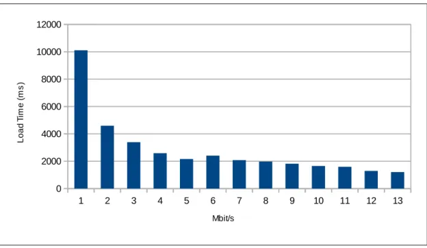
When on the other hand the bandwidth is increased as seen in Figure 8, you run into diminishing returns quickly. Already at between 4-5Mbit/s the loading times start to even out.

Figure 8: The effect of increased bandwidth on page load times

These results are very interesting, especially when considering how Internet connections are usually marketed. Bandwidth has become synonymous with speed. If you want a faster Internet experience you buy a faster (as in bandwidth) connection. These results show that delay is an important factor when discussing Internet speed.

9.2

Real-Time Response Under Load

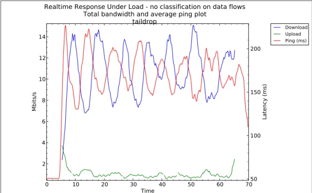
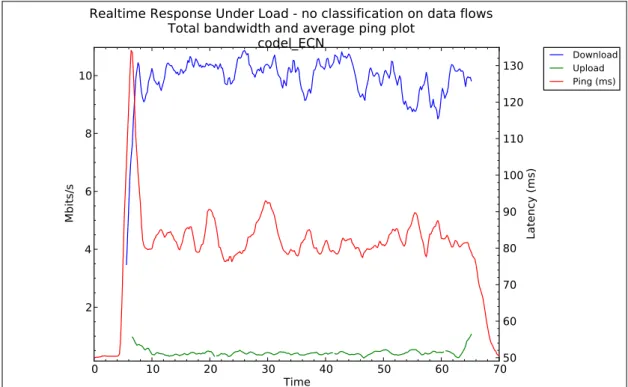
Latencies and throughput were measured while using six different queuing disci-plines. Taildrop, CoDel, FQ CoDel, PIE, ARED and SFQ. The default values for each of the algorithms were used. The first graph in each section shows the latency and packet losses while giving a rough image of the throughput[24]. The latency is measured from google.com which stays between 8-9ms under uncongested conditions. The second graph gives a more detailed look of how the latencies vary with the throughput. Here the latencies are from the test server, which is between 50-51ms under normal conditions.

9.2.1 Taildrop 2468 -240 2263 -220 2057 -200 1851 -180 1646 -160 1440 -140 1234 -120 1029 -100 823 -80 617 -60 411 -40 206 -20 0 0 -206 20 -411 40 -617 60 -823 80 -1029 100 -1234 120 -1440 140 -1646 160 -1851 180 -2057 200 -2263 220 -2468 240 P i n g t i m e ( m s ) N e t w o r k T h r o u g h p u t ( K B y t e s / s )

Ping times to host google.com correlated with packet loss and network throughput RR_D

T O O L / T O B I O E T I K E R

Bufferbloat Research Project J. Plenz / L. Ribisch / F. Ruhland

Router TX Router RX

Latency: Median (min: 8.4, max: 221.8)

Packet Loss (average: 6.1%)

(ms) Latency outliers: max: 243.9, min: 8.0

Figure 9: The median Ping time to google.com during RRUL using Taildrop

0 10 20 30 40 50 60 70 Time 2 4 6 8 10 12 14 Mbits/s Download Upload Ping (ms) 50 100 150 200 Latency (ms)

Realtime Response Under Load - no classification on data flows

Total bandwidth and average ping plot

taildrop

Local/remote: localhost.localdomain/ec2-54-77-11-144.eu-west-1.compute.amazonaws.com - Time: 2014-08-25 05:26:40.853305 - Length/step: 60s/0.20s

9.2.2 CoDel 1708 -250 1366 -200 1025 -150 683 -100 342 -50 0 0 -342 50 -683 100 -1025 150 -1366 200 -1708 250 -2049 300 -2391 350 -2732 400 P i n g t i m e ( m s ) N e t w o r k T h r o u g h p u t ( K B y t e s / s )

Ping times to host google.com correlated with packet loss and network throughput RR_D

T O O L / T O B I O E T I K E R

Bufferbloat Research Project J. Plenz / L. Ribisch / F. Ruhland

Router TX Router RX

Latency: Median (min: 8.0, max: 235.7)

Packet Loss (average: 7.8%)

(ms) Latency outliers: max: 305.0, min: 7.8

Figure 11: The median Ping time to google.com during RRUL using CoDel

0 10 20 30 40 50 60 70 Time 2 4 6 8 10 Mbits/s Download Upload Ping (ms) 50 60 70 80 90 100 110 120 130 Latency (ms)

Realtime Response Under Load - no classification on data flows

Total bandwidth and average ping plot

codel_ECN

Local/remote: localhost.localdomain/ec2-54-77-11-144.eu-west-1.compute.amazonaws.com - Time: 2014-08-25 05:55:19.569779 - Length/step: 60s/0.20s

9.2.3 FQ CoDel 1903 -30 1586 -25 1269 -20 952 -15 634 -10 317 -5 0 0 -317 5 -634 10 -952 15 -1269 20 -1586 25 -1903 30 -2220 35 -2538 40 -2855 45 -3172 50 P i n g t i m e ( m s ) N e t w o r k T h r o u g h p u t ( K B y t e s / s )

Ping times to host google.com correlated with packet loss and network throughput RR_D

T O O L / T O B I O E T I K E R

Bufferbloat Research Project J. Plenz / L. Ribisch / F. Ruhland

Router TX Router RX

Latency: Median (min: 8.4, max: 27.7)

Packet Loss (average: 0.8%)

(ms) Latency outliers: max: 48.1, min: 8.0

Figure 13: The median Ping time to google.com during RRUL using FQ CoDel

0 10 20 30 40 50 60 70 Time 2 4 6 8 10 12 Mbits/s Download Upload Ping (ms) 52 54 56 58 60 Latency (ms)

Realtime Response Under Load - no classification on data flows

Total bandwidth and average ping plot

fq_codel_ECN

Local/remote: localhost.localdomain/ec2-54-77-11-144.eu-west-1.compute.amazonaws.com - Time: 2014-08-25 05:42:36.490294 - Length/step: 60s/0.20s

Figure 14: Throughput and latencies to the test server during RRUL using FQ CoDel

9.2.4 PIE 1963 -300 1636 -250 1309 -200 982 -150 654 -100 327 -50 0 0 -327 50 -654 100 -982 150 -1309 200 -1636 250 -1963 300 -2290 350 -2618 400 P i n g t i m e ( m s ) N e t w o r k T h r o u g h p u t ( K B y t e s / s )

Ping times to host google.com correlated with packet loss and network throughput RR_D

T O O L / T O B I O E T I K E R

Bufferbloat Research Project J. Plenz / L. Ribisch / F. Ruhland

Router TX Router RX

Latency: Median (min: 8.8, max: 255.0)

Packet Loss (average: 11.7%)

(ms) Latency outliers: max: 349.2, min: 8.2

Figure 15: The median Ping time to google.com during RRUL using PIE

0 10 20 30 40 50 60 70 Time 2 4 6 8 10 Mbits/s Download Upload Ping (ms) 60 80 100 120 140 Latency (ms)

Realtime Response Under Load - no classification on data flows

Total bandwidth and average ping plot

pie_ECN

Local/remote: localhost.localdomain/ec2-54-77-11-144.eu-west-1.compute.amazonaws.com - Time: 2014-08-25 06:09:22.558173 - Length/step: 60s/0.20s

9.2.5 ARED 2228 -120 1857 -100 1485 -80 1114 -60 743 -40 371 -20 0 0 -371 20 -743 40 -1114 60 -1485 80 -1857 100 -2228 120 -2599 140 -2970 160 -3342 180 -3713 200 P i n g t i m e ( m s ) N e t w o r k T h r o u g h p u t ( K B y t e s / s )

Ping times to host google.com correlated with packet loss and network throughput RR_D

T O O L / T O B I O E T I K E R

Bufferbloat Research Project J. Plenz / L. Ribisch / F. Ruhland

Router TX Router RX

Latency: Median (min: 8.1, max: 107.2)

Packet Loss (average: 14.7%)

(ms) Latency outliers: max: 159.3, min: 7.8

Figure 17: The median Ping time to google.com during RRUL using RED

0 10 20 30 40 50 60 70 Time 2 4 6 8 10 12 Mbits/s Download Upload Ping (ms) 60 80 100 120 140 Latency (ms)

Realtime Response Under Load - no classification on data flows

Total bandwidth and average ping plot

red_ECN

Local/remote: localhost.localdomain/ec2-54-77-11-144.eu-west-1.compute.amazonaws.com - Time: 2014-08-25 10:17:15.274872 - Length/step: 60s/0.20s

9.2.6 SFQ 1903 -100 1713 -90 1523 -80 1332 -70 1142 -60 952 -50 761 -40 571 -30 381 -20 190 -10 0 0 -190 10 -381 20 -571 30 -761 40 -952 50 -1142 60 -1332 70 -1523 80 -1713 90 -1903 100 -2094 110 -2284 120 P i n g t i m e ( m s ) N e t w o r k T h r o u g h p u t ( K B y t e s / s )

Ping times to host google.com correlated with packet loss and network throughput RR_D

T O O L / T O B I O E T I K E R

Bufferbloat Research Project J. Plenz / L. Ribisch / F. Ruhland

Router TX Router RX

Latency: Median (min: 8.6, max: 90.9)

Packet Loss (average: 0.0%)

(ms) Latency outliers: max: 118.3, min: 8.5

Figure 19: The median Ping time to google.com during RRUL using SFQ

0 10 20 30 40 50 60 70 Time 2 4 6 8 10 12 Mbits/s Download Upload Ping (ms) 50 60 70 80 90 100 110 120 Latency (ms)

Realtime Response Under Load - no classification on data flows

Total bandwidth and average ping plot

sfq_ECN

Local/remote: localhost.localdomain/ec2-54-77-11-144.eu-west-1.compute.amazonaws.com - Time: 2014-08-25 06:14:41.699125 - Length/step: 60s/0.20s

9.2.7 Comparison

Taildrop performed worst in all categories. It created long delays and large amounts of jitter and Global Synchronization is clearly visible in Figure 10. Worth mentioning is that since no traffic shaping was performed, it shows a slightly larger average throughput than the rest.

Download Upload Ping (ms)

0 5 10 15 20 Mbits/s codel_ECN fq_codel_ECN pie_ECN red_ECN sfq_ECN taildrop 50 100 150 200 250 Latency (ms)

Realtime Response Under Load - no classification on data flows

Box plot of totals

Local/remote: localhost.localdomain/ec2-54-77-11-144.eu-west-1.compute.amazonaws.com - Time: 2014-08-25 05:55:19.569779 - Length/step: 60s/0.20s

Figure 21: Box plot of total Upload speed, Download speed and Ping times. The values inside the box represent 50% of the values with the red line being the median value while the values within the whiskers represent 25% each. The plus-signs represent the outliers.

All five algorithms were able to lower the delays when compared to Taildrop. The best results were had by FQ CoDel. Since the flows are separated and each get their own CoDel instance, the algorithm can focus and make decisions based on the characteristics of a single flow. The FQ part of the algorithm provide byte-level fairness between flows based on the quantum while the DRR mechanism mix the traffic flows. Thanks to these properties it was able to keep utilization high with few packet drops and low latencies.

CoDel and PIE performance were similar. Both PIE and CoDel had trouble keeping the latencies down in the beginning of the tests. After the initial spike, CoDel manages to keep even utilization and latencies while PIE had some oscillating traffic patterns. Considering the similarities, it is possible that a FQ version of PIE would perform similar to FQ CoDel.

ARED managed the highest throughput but also the highest delays. This might be because the bandwidth shaping was configured manually as opposed to the scripts used by the GUI. The ARED testing was plagued by packet drops which caused the graphing tools to misbehave and made getting consistent results difficult. The large red rectangle in Figure 17 should be ignored and the graph is mainly included as a reference.

SFQ managed to lower the delay with no packet loss as show in Figure 19 . But in Figure 20 there are a lot of missing code points in the upload, indicating packet loss. Since SFQ is only a packet scheduler, the queue length or delay caused is not managed. 50 100 150 200 250 300 Latency (ms) 0.0 0.2 0.4 0.6 0.8 1.0 Cumulative probability Ping (ms) - codel_ECN Ping (ms) - fq_codel_ECN Ping (ms) - pie_ECN Ping (ms) - red_ECN Ping (ms) - sfq_ECN Ping (ms) - taildrop

Realtime Response Under Load - no classification on data flows

ICMP CDF plot

Local/remote: localhost.localdomain/ec2-54-77-11-144.eu-west-1.compute.amazonaws.com - Time: 2014-08-25 05:55:19.569779 - Length/step: 60s/0.20s

Figure 22: Cumulative Distribution Function (CDF) used to compare latencies. The graph show how probable it is that a certain latency is present in the measurement.

9.2.8 ECN

During testing, ECN was enabled at both endpoints and the router. All the tests were also performed with ECN support turned off everywhere but no measurable difference in throughput and latency were detected.

Even though ECN goes hand in hand with an AQM, enabling it does not do much in the real world seeing as it requires support not just by the network equipment but also by both endpoints. ECN support was introduced to the Windows operating systems in Windows Server 2008 and Windows Vista but it is disabled by default. It is also disabled by default in OS X. As previously mentioned, server mode ECN (ECN only used if requested on incoming connections) is enabled by default in the Linux kernel since 2009.

A study made in 2011 showed that of the 1 million most popular websites (according to Alexa) only 12.7% use ECN markings.[25] This is an improvement compared to an earlier study from 2008 where only 1.07% supported ECN, and in the year 2000, around 8% of web servers would even refuse connections from ECN capable clients.[26]

Nowadays there should be no harm in enabling ECN, and it will help reduce packet loss and avoid retransmissions if supported.

9.3

Recommendations

The recommendations based on the facts and results presented in this thesis perfectly mirror those proposed in the current draft of the IETF recommendations for AQM.[27] An AQM system should be implemented at the consumer network edge to help reduce Bufferbloat. This should be completely transparent to the user and should therefore require no configuration. Ideally ECN would be used but this would require support at the endpoints.

9.4

Problems during testing

As this is a relatively fresh subject, implementing these solutions require some technical expertise, even for testing purposes. The CeroWRT project is currently limited to just a few routers which presented a problem in the beginning of the work. In the beginning of the project, the WNDR3700v1 was available and prepared to

be used for testing. Then when the time came to start experimenting it turned out that it was the WNDR3700v2 version that was supported. As the only difference was that the v2 had twice the flash memory, effort was put into trying to compile CeroWRT with a smaller size. Unfortunately the build system failed repeatedly during compilation. Part of the problem was that the package repositories were being migrated to a new site which lead to a lot of version discrepancies and compile errors. Previous experience of compiling OpenWRT were of no help as CeroWRT had a slightly different build procedure using scripts which might have exacerbated the issues. In the end a new router was acquired, the WNDRMACv2, with both twice the flash memory and RAM.

The ARED algorithm is not included in the CeroWRT SQM GUI and had to be configured manually. This might have been the cause of the large packet losses during testing. This also made graphing the results hard as the script collecting the data threw up errors and sometimes segmentation faults during large packet losses.

The SFQ results seem weird considering the lack of packet loss, even though the results were reproducible both with and without ECN.

9.4.1 Further Work

Since FQ CoDel has such a large advantage over a single CoDel or PIE queue, it would be very interesting to test a FQ version of PIE. It has been mentioned in mailing list discussions and talks[28] but no public version is currently available.

This work only performed measurements on unmarked traffic. This was done to provide the fairest comparison since not all applications will/can be accurately marked. But there are application that need close to guaranteed 0 packet loss and it would be interesting to see how the CoDel and PIE algorithms would perform under schemes such as Class Based Queuing (CBQ) and weight based algorithms.

It would also be interesting to perform further testing on other routing platforms and hardware.

10

Conclusion

A thorough examination of four Active Queue Management techniques has been performed. The results show that AQM in general provides better performance using both delay and throughput as a metric than no queue management. While AQM is just one part in the battle against Bufferbloat, it provides a large measurable difference and most importantly a noticeable difference for the user.

The AQM that had the best results in the tests performed during this thesis work was FQ CoDel. In itself it fulfills the criteria of a ”no knobs” and high performance AQM, making it a good fit as a default AQM in a consumer router. Even thought FQ CoDel performs well when implemented in software, an implementation of the CoDel algorithm in hardware would increase its attractiveness even further. Especially in larger networks.

While FQ CoDel is included in the Linux kernel and doesn’t need CeroWRT specifically, it still requires some configuration to get it working on your average (Linux-based) home router. It is also not zero-configuration when you consider that the modem, both for cable and DSL, is usually separate from the router. Since these modems are often very basic, and seldom have alternative firmwares available, they are out of reach for queue management. This requires traffic shaping at the router to ensure that the bottleneck is placed in the router. This is an extra step that defeats the ”no knobs” goal. This is also quite resource-intensive in Linux and might limit the total throughput. Further testing would be recommended to be done using routers with a built-in modem. This might be difficult as firmware support for the modem hardware is often sparse.

But the main problem is the lack of awareness. A large-scale push for AQM would need the full support of the Internet community, equipment manufacturers and Internet Service Providers. Since AQM benefits everyone, this will hopefully not present a large hurdle.

11

Summary

To satisfy the demands of todays Internet users, ISPs have to provide both high throughput and low delays. Service providers use bandwidth as a selling point while delays are largely ignored.

Bufferbloat is the cause of most delays experienced by users. Bufferbloat is caused by overly large buffers and unmanaged queues in networking equipment. The equipment available for purchase or provided by the ISP is ill-equipped to deal with this problem.

Three different proposed solutions to the Bufferbloat problem have been de-scribed and tested. The work on CoDel and FQ CoDel which came out of the Bufferbloat project and PIE from Cisco. A test-setup consisting of a home-router on a residential DSL-connection was set up to evaluate the solutions. The delay experienced by traffic flows while the router was under heavy load to try to in-duce Bufferbloat was measured, first using no queue management and then the three queue management algorithms. All three provided lower delays and high throughput with FQ CoDel coming out on top. The ARED AQM and the packet scheduler SFQ were also included as references.

The conclusion reached is that some sort of AQM should be implemented at the network edge. While still under development, FQ CoDel seems like a very promising AQM to use against Bufferbloat.

12

References

[1] John Nagle. Congestion control in ip/tcp internetworks. Request For Com-ments RFC896, IETF, January 1984.

[2] John Nagle. On packet switches with infinite storage. Request For Comments RFC970, IETF, December 1985.

[3] Jim Gettys and Kathleen Nichols. Bufferbloat: Dark buffers in the internet. Queue, 9(11):40:40--40:54, November 2011. URL: http://doi.acm.org/10.

1145/2063166.2071893, doi:10.1145/2063166.2071893.

[4] CACM Staff. Bufferbloat: What’s wrong with the internet? Commun. ACM, 55(2):40--47, February 2012. URL: http://doi.acm.org/10.1145/2076450. 2076464, doi:10.1145/2076450.2076464.

[5] Bufferbloat project, August 2014. URL: http://www.bufferbloat.net. [6] Van Jacobson, Kathy Nichols, Kedar Poduri, et al. Red in a different light,

1999.

[7] Kathleen Nichols and Van Jacobson. Controlling queue delay. Commun. ACM, 55(7):42--50, July 2012. URL: http://doi.acm.org/10.1145/2209249. 2209264, doi:10.1145/2209249.2209264.

[8] V. Jacobson K. Nichols. Controlled delay active queue management. Internet Draft draft-nichols-tsvwg-codel-02, IETF, March 2014.

[9] T. Hoeiland-Joergensen at al. Flowqueue-codel. Internet Draft draft-hoeiland-joergensen-aqm-fq-codel-00, IETF, March 2014.

[10] Rong Pan, P. Natarajan, C. Piglione, M.S. Prabhu, V. Subramanian, F. Baker, and B. VerSteeg. Pie: A lightweight control scheme to address the bufferbloat problem. In High Performance Switching and Routing (HPSR), 2013 IEEE 14th International Conference on, pages 148--155, July 2013. doi:10.1109/

HPSR.2013.6602305.

[11] R. Pan et al. Pie: A lightweight control scheme to address the bufferbloat problem. Internet Draft draft-pan-aqm-pie-01, IETF, februari 2014.

[12] Y. Gong, D. Rossi, C. Testa, S. Valenti, and M.D. T¨aht. Fighting the bufferbloat: On the coexistence of {AQM} and low priority conges-tion control. Computer Networks, 65(0):255 -- 267, 2014. URL: http:// www.sciencedirect.com/science/article/pii/S1389128614000188, doi: http://dx.doi.org/10.1016/j.bjp.2014.01.009.

[13] Toke Høiland-Jørgensen. Battling bufferbloat: An experimental comparison of four approaches to queue management in linux. Master’s thesis, Roskilde University, 2012.

[14] Greg White and Dan Rice. Active queue management algorithms for docsis 3.0. Cable Television Laboratories, Inc, 2013.

[15] L. Eggert et al. Unicast udp usage guidelines for application designers. Best Current Practice RFC5405, IETF, Novemeber 2008.

[16] V. Jacobson et al. Tcp extensions for high performance. Proposed Standard RFC1323, IETF, May 1992.

[17] M. Allman et al. Tcp congestion control. Draft Standard RFC5681, IETF, September 2009.

[18] M. Mathis et al. Tcp selective acknowledgment options. Proposed Standard RFC2019, IETF, October 1996.

[19] K. Ramakrishnan et al. The addition of explicit congestion notification (ecn) to ip. Proposed Standard RFC3168, IETF, September 2001.

[20] Sally Floyd and V. Jacobson. Random early detection gateways for congestion avoidance. Networking, IEEE/ACM Transactions on, 1(4):397--413, Aug 1993. doi:10.1109/90.251892.

[21] Sally Floyd, Ramakrishna Gummadi, Scott Shenker, et al. Adaptive red: An algorithm for increasing the robustness of red’s active queue management. Preprint, available at http://www. icir. org/floyd/papers. html, 2001.

[22] C.V. Hollot, V. Misra, D. Towsley, and W.-B. Gong. On designing im-proved controllers for aqm routers supporting tcp flows. In INFOCOM 2001.

Twentieth Annual Joint Conference of the IEEE Computer and Communica-tions Societies. Proceedings. IEEE, volume 3, pages 1726--1734 vol.3, 2001. doi:10.1109/INFCOM.2001.916670.

[23] Little’s law. Wikipedia, August 2014. URL: http://en.wikipedia.org/ wiki/Little%27s_law.

[24] Rrd graphing tool, August 2014. URL: http://git.plenz.com/ bufferbloat/tree/graph.

[25] Steven Bauer et al. Measuring the current state of ecn support in servers, clients, and routers, February 2011. URL: http://www.caida.org/workshops/isma/ 1102/slides/aims1102_sbauer.pdf.

[26] Dax Kelson. 8% of the internet unreachable!, September 2000. URL: http: //lkml.iu.edu//hypermail/linux/kernel/0009.1/0329.html.

[27] F. Baker et al. Ietf recommendations regarding active queue management. Internet Draft draft-ietf-aqm-recommendation-08, IETF, August 2014. [28] Rong Pan. A follow up on the pie queue management algorithm 86th

ietf, March 2013. URL: http://www.ietf.org/proceedings/86/slides/ slides-86-iccrg-5.pdf.