Department of Forest Resource Management
Assessing the accuracy for area-based tree
species classification using Sentinel-1
C-band SAR data
Alberto Udali
Master Thesis project • 30 credits
Master Thesis in Forest Science
Arbetsrapport / Sveriges lantbruksuniversitet, Institutionen för skoglig resurshushållning,• 504 • ISSN 1401-1204
Assessing the accuracy for area-based tree species
classifi-cation using Sentinel-1 C-band SAR data
Alberto Udali
Supervisor: Henrik Persson, Swedish University of Agricultural Sciences, De-partment of Forest Resource Management
Assistant supervisor: Eva Lindberg, Swedish University of Agricultural Sciences, Depart-ment of Forest Resource ManageDepart-ment
Examiner: Johan Fransson, Swedish University of Agricultural Sciences, De-partment of Forest Resource Management
Credits: 30 credits
Level: A2.E
Course title: Master Thesis in Forest Science
Course code: EX0921
Programme/education: Forest Science
Course coordinating department: Department of Forest Resource Management
Place of publication: Umeå Year of publication: 2019
Title of series: Arbetsrapport / Sveriges lantbruksuniversitet, Institut-ionen för skoglig resurshushållning
Part number: 504
ISSN: 1401-1204
Online publication: https://stud.epsilon.slu.se
Keywords: Sentinel-1, tree species, random forest, linear discrimi-nant analysis, classification
Forest type (FTY) and tree species classification (SPP) over the Remn-ingstorp test site were performed using ground-based field observations and remote sensing data sources. The field inventory for the forest estate and for the surrounding natural reserve of Eahagen was carried out in 2016. The re-mote sensing data used were C-band Synthetic Aperture Radar (SAR) data from Sentinel-1. Dual polarization backscatter values were extracted for the period October 2017 - February 2019 and the area-based method was applied. The metrics obtained, i.e. monthly mean backscatter, were used to perform classification by machine learning models’ random forest (RF) and linear dis-criminant analysis (LDA). The models were evaluated with the leave-one-out cross-validation method and the classification outcomes were compared with reference values in terms of confusion matrixes. The best performing model was LDA with an overall accuracy of 88% for FTY and 61% for SPP, whereas RF achieved values of 84% for FTY and 56% for SPP. It was concluded that C-band SAR data can be used for FTY and SPP classification, but further investigation is needed to determine which factors affect the backscatter in order to obtain more accurate classifications.
Keywords: Sentinel-1, tree species, random forest, linear discriminant analysis,
classification
List of Tables 7 List of Figures 8 1 Introduction 9 1.1 Background 9 1.2 Previous studies 11 1.3 Research questions 12
2 Materials and Methods 13
2.1 Study area 13 2.2 Field data 14 2.3 Satellite data 16 2.4 Data extraction 18 2.5 Multi-temporal images 19 2.6 Methods of classification 23 2.7 Accuracy assessment 24 3 Results 26 3.1 Random Forest 26
3.2 Linear Discriminant Analysis 28
4 Discussion 30
5 Conclusions 34
References 36
Appendix 41
Table 1: Tree species considered in the study. 15
Table 2: IW-GRD images specifications. 18
Table 3: Number of acquisitions per time frame. 18
Table 4: Variance values for the VH-polarization mean backscatter (dB) for each class. 22
Table 5. Confusion matrix combinations. 25
Table 6: Overall accuracy values for FTY and SPP. 26
Table 7: RF3-VH VV confusion matrix. 27
Table 8: RF5-VH VV confusion matrix. 27
Table 9: Overall accuracy values for FTY and SPP. 28
Table 10: LDA3-VH VV confusion matrix. 28
Table 11: LDA5-VH VV confusion matrix. 29
Table 12: Confusion matrix for Coniferous and Deciduous classification. 31 Table 13: Results comparison with previous studies in the literature. 31
Table A. 1: RF3-VH. 41 Table A. 2: RF3-VV. 41 Table A. 3: RF5-VH. 41 Table A. 4: RF5-VV. 42 Table A. 5: LDA3-VH. 42 Table A. 6: LDA3-VV. 42 Table A. 7: LDA5-VH. 43 Table A. 8: LDA5-VV. 43
List of Tables
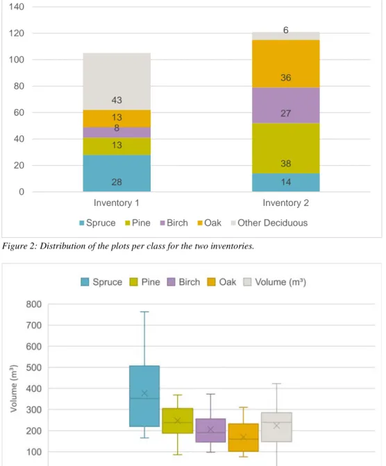
Figure 1: Location and map of the study area. 14 Figure 2: Distribution of the plots per class for the two inventories. 16 Figure 3: Illustration of the spread in volume for the same species but for different plots in
Inventory 1. 16
Figure 4: Schematic of the mean value extraction for each raster stack. 19 Figure 5: Backscatter trend through the time series. 20 Figure 6: Backscatter trend for the deciduous species. 21 Figure 7: Backscatter trend for the coniferous species. 21 Figure 8: Illustration of the spread in backscatter for the same species but for different plots
for February 2018. 22
Figure 9: Illustration of the spread in backscatter for the same species but for different plots
for February 2019. 23
Figure 10: Comparison of the overall accuracy results. 29
1.1 Background
Monitoring natural resources and how these are used and exploited is fundamental in today’s world, e.g., common-pool resources such as water systems, the global atmosphere and forests (Ostrom, 2009). At global level one of the main interests of forests is to know the status and the extent of those, as well as the biomass and the main forest type. In order to keep these kind of information updated, the role of satellite images is crucial to monitor the land use and changes (Nemani and Running, 1996). At local level (regional or property) more detailed information is necessary to assess the status of a forest, and some pieces are provided by National Forest Inventories (NFIs) and, at property level, by management plans.
Forest species composition is important when assessing, e.g., forest biodiversity which includes diversity within species and between species, and ecosystems con-sidering also functions and processes, structures and services (Innes and Koch, 1998). It can become significant for forest owners that are interested in game and hunting to know what tree species are prevalent in their property that might attract more wildlife and adjust those proportions according to the management strategies for their properties. On the other hand, knowing the forest composition can influ-ence the management plan in a significant way when dealing with biodiversity and conservation purposes (Lindenmayer et al., 2000), leading to good practices known as Sustainable Forest Management. As reported by the Forest Resources Assess-ment in 2015, although the public interest is still focused on forest change, e.g., degradation and deforestation, many other forests have changed in other ways, not immediately visible to the general public, such as in composition and density, and climate change is predicted to create substantial shifts in tree species distribution
future. The species composition of a forest will then influence its future composition and how the landscape and ecosystem will respond and look in the future; knowing a forest’s actual composition can greatly influence the management solutions when dealing with natural dynamics and climate change dynamics (Gustafson and Keene, 2014).
The use of remote sensing (RS) techniques in forestry has developed during the last decade or two when it comes to obtain information about forests over a large scale (i.e., the Amazonian forest or the Boreal shield) and keep those information updated, not only to assess quantitative variables such as the more classic forest parameters, height (H), volume (VOL), basal area (BA), diameter (D), above-ground biomass (AGB), but also to estimate more qualitative data such as species biodiversity (Innes and Koch, 1998), habitat loss and degradation, climate change effects and the spread of invasive species (Pettorelli et al., 2014). As for forestry, RS based images have been used since the 1940s with mainly the application of stereo-photogrammetry from aerial images (Korpela, 2004), but nowadays more data are becoming available and accessible from other sources. Airborne RS can provide, together with aerial photo-interpretation and field sampling, precise and reliable information on forests. Moreover, airborne sources can provide ecologically important parameters (e.g., LAI), improved accuracy for species composition, canopy cover and gap closure (King, 2000). In areview paper by Yu et al. (2015), they provide a solid comparison between different RS sources when used to retrieve forest parameters (i.e., AGB, VOL, BA, D and H)at plot level. In the paper they confirm that measurements con-ducted via RS-based information can range their performances from quite accurate to very accurate overall. Therefore, not all RS sources are apparently suitable to retrieve the same type of information: e.g., space borne images can cover larger areas, if compared to airborne images.
The number of tree species classification studies using RS has increased over the last 40 years, with focus on the use of laser data and optical multispectral systems, or the two combined, compared with the use of radar to separate tree species (Fassnacht et al., 2016). This is mainly because of the better accuracy (Yu et al., 2015) that the data provide, or even though because used for longer time, e.g., in the case of aerial stereo-photogrammetry. Nevertheless, the increasing and renewed in-terest in using Radio Detection and Ranging (RADAR) data related to forestry and species classification is addressed as one of the challenges for future studies.
1.2 Previous studies
Synthetic aperture RADAR (SAR) is used to create two-dimensional images or three-dimensional reconstructions of objects, such as landscapes (Kirscht and Rinke, 1998), and it is the most used type of data when dealing with forest. The majority of the SAR studies related to forestry are focused on the discrimination between broad forest types, associated to land cover classification, rather than to species level. The information provided by SAR are mainly related to the canopy structure and its water content (Fassnacht et al., 2016).
This kind of information related to the behavior of the canopy, how the different elements interact with the signal can be assessed and quantified by the radar backscatter. This can be influenced by two main kind of factors: one category is related to the instrument and the other is related to the scattering objects. Several authors report about the different interactions between canopy architecture and the backscatter. Dostálová et al. (2016) report how the signal reflection is affected by the different species branch geometry and canopy structure. Also, the leaves shape can provide information to facilitate the separation of species (Rignot et al., 1994). Moreover, not only the specific crown architecture has a strong influence, but as well can be said for the different phenology of tree species. Frison et al. (2018) demonstrated that there is a visible correlation between the radar backscatter coef-ficient between polarizations and seasonality, and this is especially related to the phenology of the different species. Furthermore, Rüetschi, et al. (2018), proved that there is an opposite behavior between coniferous and deciduous trees regarding an-nual monitoring of the backscatter in winter and summer, i.e. leaf-on and leaf-off conditions.
Concerning the species classification, this can produce overall good results with different techniques (Santoro et al., 2017). More success has been achieved through classification of forest types compared to single species. Dostálová, et al. (2018) reached an overall accuracy of 85% when classifying the forest type (between non-forest, coniferous and broadleaf forest classes) in temperate non-forest, and their estima-tions decreased to 65% for boreal forests. Although not having the same type of classification, Rüetschi et al. (2018) achieved a similar overall accuracy (86%) in a similar scenario, with comparable characteristics. Even though using a different ra-dar source such as GF-3 and POLSAR, Zhou et al. (2018) report about a forest type classification run in Northern China between four forest classes (coniferous, broad-leaf, mixed and other forest) with an overall accuracy of 90%.
1.3 Research questions
The objective of this thesis is to evaluate the radar backscatter for tree species clas-sification by assessing the accuracy for area-based tree species clasclas-sification using C-band SAR data, and if a more detailed type of classification among different spe-cies inside a stand can be reliable and accurate, and to which extent.
2.1 Study area
The study area selected is the Remningstorp forest estate and the nearby nature re-serve Eahagen in southern Sweden (58°30’N, 13°40’E). According to the estate management plan of 2008, the prevailing tree species in the area are Norway Spruce (Picea abies L.), Scots Pine (Pinus sylvestris L.) and Birch (Betula spp.), with a minor presence of other deciduous species. The estate has been used as a test site for SLU since the mid 1980s.
Eahagen is a natural reserve neighboring the estate and is rich in biodiversity for broadleaves tree species. The main species present in the area are Pedunculate Oak (Quercus robur), Wych Elm (Ulmus glabra), Norway Maple (Acer platanoides), Small-Leaved Lime (Tilia cordata), European Ash (Fraxinus excelsior), Hornbeam (Carpinus betulus), and in less proportion there might be found also Wild Cherry (Prunus avium), Alder (Alnus glutinosa), Betula spp. and Aspen (Populus tremula).
Figure 1: Location and map of the study area.
2.2 Field data
The field inventory on Remningstorp was carried out in 2016. The sampling design was systematic sampling out of a random starting point with field plots placed out in a grid to ensure a representative sample of the species composition on the estate. This dataset is mainly constituted of Norway Spruce, Scots Pine and Birch. An ad-ditional inventory was carried out in the adjacent nature reserve Eahagen to com-plement the dataset with broadleaf tree species. For this inventory, the location of the plots’ center was flexible, since the aim of the inventory was to find plots that were dominated by a single tree species within homogenous stands (Lindberg 2017; Persson et al., 2018). The plots were then reviewed individually and only the ones with at least 80% in volume of the same species were kept (Goncalves, 2017). The plots which did not fulfil this requirement were not used.
The field data in the present study was less extensive for some of the classes con-sidered, and therefore additional subjective plots were manually placed to gain suf-ficiently number of plots per tree species (Rogan et al., 2010; Olofsson et al., 2014). The plots and data concerning the second dataset were included to supplement the less represented classes. The forest management plan of Remningstorp was queried for stands that were constituted of at least 80% of the target species and where the
total volume was more than 200 m3. Within these stands, plots were placed out
sub-jectively using volume and species distribution as reference with support of aerial photos. The centers of the plots were located in areas of the stands dominated by a single tree species. Moreover, the points were put with more than 30 m between each other, since each observation was then used to build a buffer of 12 m to use for the extraction of the backscatter.
The species targeted in this study are listed in Table 1 and regrouped into the forest type (FTY) and into species (SPP) categories for the two classifications.
Table 1: Tree species considered in the study.
Tree species Scientific name FTY SPP
Norway Spruce Picea abies L. Coniferous Spruce Scots Pine Pinus sylvestris L. Coniferous Pine
Birch Betula spp. Deciduous Birch
Ash Fraxinus excelsior Deciduous Other Deciduous
Alder Alnus glutinosa Deciduous Other Deciduous Aspen Populus tremula Deciduous Other Deciduous
Oak Quercus robur Deciduous Oak
The distribution of the plots among the two inventories is shown in Figure 2. The first inventory, from Lindberg (2017), is shown as Inventory 1 and the second one, placed with aerial photo-interpretation, is called Inventory 2. A total of 226 plots were used, 105 belonging to Inventory 1 and 121 to Inventory 2.
The backscatter signal can be strongly influenced by the stem volume, therefore the saturation threshold of 200 m3 was established, to minimize the effect to which the
C-band SAR backscatter is subjected (Santoro et al., 2013; Sinha et al., 2015; Huang et al., 2018). In Figure 3, the volume distribution according to the different species present in Inventory 1 is reported. SAR backscatter is also predicting stem volume, therefore, it is important that all species have plots from almost the entire range of stem volumes. Hence, this guarantees that the methods used will not learn classifi-cation due to volume influence instead of species’ own backscatter.
Figure 2: Distribution of the plots per class for the two inventories.
Figure 3: Illustration of the spread in volume for the same species but for different plots in Inventory 1.
2.3 Satellite data
RADAR data have been used in research related to forestry since the 1990s at least (Benallegue et al., 1995), but more continuous information has been available since
28 14 13 38 8 27 13 36 43 6 0 20 40 60 80 100 120 140 Inventory 1 Inventory 2
the start of the more recent space programs, like the Sentinel program from the Eu-ropean Space Agency (ESA) in 2014, making possible to build observations based on time series of images.
The Sentinel-1 mission is composed of a constellation of two satellites, Sentinel-1A and Sentinel-1B, which share the same orbit; both of them carry a C-band Synthetic Aperture Radar (SAR) instrument collecting data continuously, day and night, in all-weather conditions, providing data in dual polarization capability. Each satellite has an orbit of 12 days and the instruments can work with different resolution (down to 5 m) and coverage (up to 400 km). The first satellite, Sentinel-1A, was launched on April 2014 and the Sentinel-1B was launched on April 2016. The 12-days orbit of the two satellites permits to have new data and radar images every 6 days in average since the two instruments share the same orbit but 180° phase shifted, al-lowing the continuous land monitoring.
In order to understand the backscatter behavior of different tree species, a multi-seasonal time series of SAR acquisitions was selected. Multiple SAR images grouped into a time series can reveal temporal signatures (Rüetschi et al., 2018) and monitor the phenology of the species (Ahern et al., 1993; Proisy et al., 2000). Sen-tinel-1 acquisitions were taken from October 2017 to February 2019 from the Co-pernicus Hub platform and processed in the Sentinel Application Platform (SNAP) from ESA (ESA, 2014). SNAP is an open source common architecture for ESA Toolboxes ideal for the exploitation, processing and analysis of Earth Observation data.
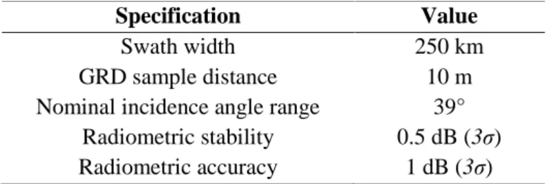
With the purpose of avoiding the backscatter to be influenced by the different factors related to the instrument, such as the frequency of the wavelength, the polarization and the incidence angle, images from the same satellite orbit were taken for the whole considered period. The orbit considered over the study area was No. 73 and the acquisition mode used was the Interferometric Wide Swath (IW). With this method the satellite captures three sub-swaths using Terrain Observation with Pro-gressive Scans SAR (TOPSAR) technique, which helps to build an homogeneous quality image throughout the whole swath (De Zan and Monti Guarnieri, 2006). Ground Range Detected (GRD) data were used, multi-looked and projected to ground range using Earth ellipsoid WGS84. In Table 2 the IW-GRD specifications are listed.
Table 2: IW-GRD images specifications.
Specification Value
Swath width 250 km GRD sample distance 10 m Nominal incidence angle range 39°
Radiometric stability 0.5 dB (3σ) Radiometric accuracy 1 dB (3σ)
Compared to previous studies, the following approach was used; to best cover the considered period, different time frames were taken in consideration (February 2018 and 2019, May 2018, August 2018 and October 2017 and 2018) and all available acquisitions for those were used. Only these time frames were considered because these were the ones that would enhance the different backscatter behavior between coniferous and deciduous trees (Dostálová et al., 2016; Dostálová et al., 2018). For each image, both polarizations were used (VH and VV). In total, 31 images were downloaded and processed in SNAP. In Table 3 the number of images included in each time frame is reported.
Table 3: Number of acquisitions per time frame.
Time frame No. of acquisitions
October 2017 5 February 2018 5 May 2018 5 August 2018 5 October 2018 6 February 2019 5 Total 31
2.4 Data extraction
The main methodology applied to this case study could be described as an applica-tion of the area-based method, explained in the paper by White et al. (2013). Gen-erally, the method consists of two stages. In the first stage, data from the remote sensing source are acquired for the entire area of interest. Measures at tree-level are carried out in the sample plots and predictive or classification models are developed. In the second stage, the models are applied for the entire raster based on the data obtained in the first stage.
2.5 Multi-temporal images
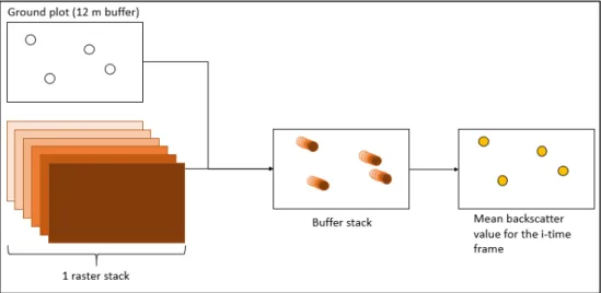
In a first step, all SAR acquisitions were calibrated and geocoded (Figure 4). These operations were run in the SNAP application and, at the end, a raster file of the backscatter signal (in dB) was saved for each image.
The average backscatter value for the plots was extracted using the statistical soft-ware R. All the information collected through the field survey for the plots, is valid for the buffer area in which the plot is included. After correcting the extent and co-registered the images, six raster stacks were built, one for each time frame. These raster stacks, consisting in a collection of raster layer objects with the same spatial extent and resolution, were used as temporary list of files to store the data and used for both SAR polarizations. These operations were performed separately for the VH-polarization and then for the VV-VH-polarization. Each stack was then clipped to the buffer polygon and the mean backscatter values were extracted for each buffer (Fig-ure 4). After this, a monthly mean was calculated as representative for the entire time frame, resulting in a total of six means for all the 226 plots (Figure 5).
Figure 5: Backscatter trend through the time series.
It is possible to see that the two polarizations contribute in different ways to describe the backscatter; where the VV does not show any particular variation throughout the whole time period considered, the VH shows some differences through time. More-over, the variation between VV-values appears to be lower than the variation among the VH-values. Overall, a drop in the backscatter signal can be observed in February 2018 and can be found both in VV and VH, but does not seem to be cyclical since it is not repeating in February 2019.
It is reasonable to assume that the VH-polarization carries the majority of infor-mation useful to achieve a correct classification, as pointed out by Dostálová et al. (2018). In Figure 6, the VH-polarization for the deciduous species listed in Table 1 and their backscatter in the time period is reported.
-19 -17 -15 -13 -11 -9 -7
Oct17 Feb18 May18 Aug18 Oct18 Feb19
B ac k s c at ter ( dB ) Time (month)
Spruce VH Spruce VV Pine VH
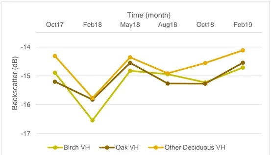
Figure 6: Backscatter trend for the deciduous species.
It is possible to appreciate where some differences in values are more pronounced. Especially in October 2017, May 2018 and in February 2019, the mean values look distinct among the three deciduous categories, but this distinction do not operate through the entire time series and do not qualify as enough to set a clean distinction, e.g., the Birch backscatter suffered a huge drop in February 2018. In Figure 7, the coniferous species are plotted; although with different mean values, the two species show similar behavior and tendency throughout time.
-17 -16 -15 -14
Oct17 Feb18 May18 Aug18 Oct18 Feb19
B ac k s c at ter ( dB ) Time (month)
Birch VH Oak VH Other Deciduous VH
-18 -17 -16 -15 -14 -13
Oct17 Feb18 May18 Aug18 Oct18 Feb19
B ac k s c at ter ( dB ) Time (month) Spruce VH Pine VH
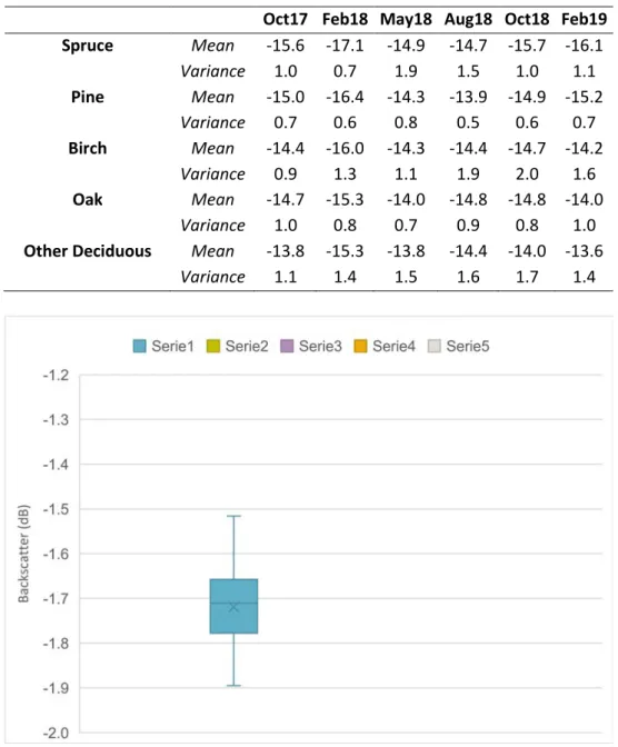
One general observation can be made by looking at the variance inside the catego-ries and how the values vacatego-ries inside the interval. In Table 4, the variance values together with the mean backscatter values for each month are reported. Moreover, from Figures 6 and 7, it is reasonable to assume that the differences between the different species are enhanced in February 2018 and February 2019. The backscatter for the two time frames has been plotted in Figures 8 and 9.
Table 4: Variance values for the VH-polarized mean backscatter (dB) for each class.
Oct17 Feb18 May18 Aug18 Oct18 Feb19
Spruce Mean -15.6 -17.1 -14.9 -14.7 -15.7 -16.1 Variance 1.0 0.7 1.9 1.5 1.0 1.1 Pine Mean -15.0 -16.4 -14.3 -13.9 -14.9 -15.2 Variance 0.7 0.6 0.8 0.5 0.6 0.7 Birch Mean -14.4 -16.0 -14.3 -14.4 -14.7 -14.2 Variance 0.9 1.3 1.1 1.9 2.0 1.6 Oak Mean -14.7 -15.3 -14.0 -14.8 -14.8 -14.0 Variance 1.0 0.8 0.7 0.9 0.8 1.0
Other Deciduous Mean -13.8 -15.3 -13.8 -14.4 -14.0 -13.6
Variance 1.1 1.4 1.5 1.6 1.7 1.4
Figure 8: Illustration of the spread in backscatter for the same species but for different plots for Feb-ruary 2018.
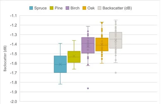
Figure 9: Illustration of the spread in backscatter for the same species but for different plots for Feb-ruary 2019.
Overall it is possible to observe that the classes’ backscatter range overlap with each other, making not clear distinction. Moreover, a single SAR monthly series of ac-quisitions is not enough to determine the tree species, but more acac-quisitions are nec-essary.
2.6 Methods of classification
The methods used to make the classification for this study were Random Forest (RF) and Linear Discriminant Analysis (LDA). The two models are listed as in the top three most used classification models in Fassnacht et al. (2016). Both methods can be run in R: RF is an ensemble method for classification and regression that operates by constructing a multitude of decision trees based on a training dataset and giving as output the mode of the classes (classification) or the mean prediction (regression) of the individual trees (Ho, 1995; Ho, 1998; Breiman, 2001). Whereas, LDA is a generalization of Fisher’s linear discriminant used to find a linear combination of features able to characterize or separate two or more classes of objects or events (Fisher, 1936; McLachlan, 1992).
𝐶𝐶𝐶𝐶𝐶𝐶𝐶𝐶𝐶𝐶 ~ 𝑥𝑥1+ 𝑥𝑥2+ ⋯ + 𝑥𝑥𝑛𝑛 (1)
Where Class is the generic expression for the two classification values (forest type or species classification), and xn describes the n-variables that have been used by the
relation to estimate the classification. What the function aims to do is to describe a qualitative attribute (tree species) based on quantitative attributes (different backscatter values through time).
2.7 Accuracy assessment
RF in RStudio was applied by first maintaining the default settings with two varia-bles tried at each split (mtry=2) and a forest size of 500 trees (ntree=500), and then tuned to improve the result by changing the number of variables to try and the num-ber of trees: the tuning process proceeds by searching the optimal value of mtry for RF that minimize the out-of-bag error (OOB), which is a method of measuring the prediction error for machine learning models that uses bagging to sub-sample the data sample used for training the mode. Then the model was trained by using the “train” function contained in the caret package for RStudio. With this, it was possi-ble to get a first estimation of the model performance based on a training set: this was generated using the leave-one-out cross-validation (LOOCV) approach. This approach was used for both models in both their training/tuning phase and in their final application. The LOOCV is a particular case of leave-p-out cross-validation with p=1. This involves using p observations as the test set and the remaining as the training set for the model.
For each model, the classifications’ outcomes were confronted with the real values and evaluated with a confusion matrix, that allowed a clear visualization of the clas-sifications’ performance of the algorithm (Stehman, 1997; Sammut and Webb, 2011). The data used to build the confusion matrix were the ones belonging to the initial dataset provided by Lindberg (2017); these were the ones systematically col-lected in the field. The second dataset, positioned using aerial photo-interpretation of the management plan, was only used to provide more information to the model to be trained for the classification. A total of twelve classifications were made, which are reported below in Table 5.
Table 5. Confusion matrix combinations.
Method Classification Polarization
used Abbreviation Random Forest FTY VV RF3-VV VH RF3-VH VH VV RF3-VHVV SPP VV RF5-VV VH RF5-VH VH VV RF5-VHVV Linear Discrimi-nant Analysis FTY VV LDA3-VV VH LDA3-VH VH VV LDA3-VHVV SPP VV LDA5-VV VH LDA5-VH VH VV LDA5-VHVV For each one of the classifications, also according to the good practices described in Olofsson et al. (2014), user’s accuracy, producer’s accuracy and overall accuracy were calculated and reported. The user’s accuracy gives a proportion for which the considered class has been either correctly classified or oversteps its bounds and clas-sifies other cover types. Essentially, the user’s accuracy describes the accuracy from the point of view of a map user and tells how often the class on the map will actually be present on the ground. The producer’s accuracy describes the ratio of the field data for the given class that was correctly classified and, hence, tells how often real features on the ground are correctly shown on the classified map or the probability that a certain land cover of an area on the ground is classified as such. Finally, the overall accuracy gives the proportion of the data correctly classified over the total number of observations.
The first subchapter describes the results obtained from the application of the RF model, the second subchapter defines the results from the application of LDA.
3.1 Random Forest
In Table 6, the overall accuracy results for applying the model to predict FTY and SPP values are reported.
Table 6: Overall accuracy values for FTY and SPP.
Overall accuracy
Polarization FTY SPP
VV 0.60 0.29
VH 0.80 0.50
VH VV 0.84 0.56
By observing the accuracy values for the different classifications, it is possible to appreciate that the VH-polarization carries most of the information useful. This is more enhanced when comparing VH FTY and SPP results. The confusion matrices of both classifications for the VH- and VV-polarization combined are reported in Tables 7 and 8. The rest of the confusion matrices produced by the RF classifications are attached in the Appendix.
Table 7: RF3-VH VV confusion matrix.
Classification
Field data Spruce Pine Deciduous Sum User’s accuracy
Spruce 18 1 3 22 0.82 Pine 6 9 0 15 0.60 Deciduous 4 3 61 68 0.90 Sum 28 13 64 105 Producer’s accuracy 0.64 0.69 0.95 Overall accuracy 0.84
The classification resulted with an overall accuracy of 0.84 and achieved high values for producer’s and user’s accuracy for the Deciduous class equal or higher than 0.90. For both the Coniferous species the values do not surpass 0.70, except for Spruce user’s accuracy that reaches 0.82.
Table 8: RF5-VH VV confusion matrix.
Classification Field data Spruce Pine Birch Oak Other
Deciduous Sum User’s accuracy Spruce 20 2 1 1 2 26 0.77 Pine 5 10 1 1 2 19 0.53 Birch 0 1 1 0 6 8 0.13 Oak 2 0 1 9 14 26 0.35 Other Deciduous 1 0 4 2 19 26 0.73 Sum 28 13 8 13 43 105 Producer’s accuracy 0.71 0.77 0.13 0.69 0.44 Overall accuracy 0.56
For the Coniferous species, both producer’s and user’s accuracy resulted in higher values than in the previous classification, except for Spruce and Pine user’s accuracy that passed from 0.82 to 0.77 and 0.60 to 0.53, respectively. From the results related to the Deciduous species, the emerging scenario is not clear and precise. The species more affected by this classification is the Birch, achieving only 0.13 for both the accuracies.
3.2 Linear Discriminant Analysis
The overall accuracy results for FTY and SPP are reported in Table 9.
Table 9: Overall accuracy values for FTY and SPP.
Overall accuracy
Polarization FTY SPP
VV 0.63 0.31
VH 0.85 0.56
VH VV 0.88 0.61
As for RF, the results from LDA show the same trend but with higher values in accuracy for both FTY and SPP. For the SPP classification using the dual-polariza-tion, the value is 5% higher than RF and reaches 0.61, which is close to the overall accuracy reached in FTY using only the VV-polarization backscatter.
As for RF, the model results and real values were computed into a confusion matrix and accuracy values were calculated. The confusion matrices for the VH- and VV-polarization are reported in Tables 10 and 11, whereas the others are attached in the Appendix.
Table 10: LDA3-VH VV confusion matrix.
Classification
Field Data Spruce Pine Deciduous Sum User’s accuracy
Spruce 20 0 0 20 1.00 Pine 3 11 3 17 0.65 Deciduous 5 2 61 68 0.90 Sum 28 13 64 105 Producer’s accuracy 0.71 0.85 0.95 Overall accuracy 0.88
Compared to RF, the classification for FTY reached a higher value in accuracy. User’s accuracy for Spruce reached 1.00. Producer’s and user’s accuracy for Decid-uous species reached the same values as with RF.
Table 11: LDA5-VH VV confusion matrix.
Classification:
Field data Spruce Pine Birch Oak Other
Deciduous Sum User’s accuracy Spruce 21 0 0 0 0 21 1.00 Pine 5 12 1 1 1 20 0.60 Birch 0 0 0 1 10 11 0.00 Oak 1 1 2 9 10 23 0.39 Other Deciduous 1 0 5 2 22 30 0.73 Sum 28 13 8 13 43 105 Producer’s accuracy 0.75 0.92 0.00 0.69 0.51 Overall accuracy 0.61
The accuracy results for the Coniferous species maintained the same trend shown for FTY, with Pine producer’s accuracy increasing to 0.92. As pointed out for SPP classification with RF, the classification among the Deciduous species has not shown extremely good results in producer’s accuracy. Different plots have been mis-classified into Other Deciduous instead of their correct value (Birch and Oak), but overall the same for RF SPP and LDA SPP. The overall accuracy values of all the classification performed, showed in Tables 6 and 9, are compared and plotted in Figure 10. 60% 63% 29% 31% 80% 85% 50% 56% 84% 88% 56% 61% 0% 10% 20% 30% 40% 50% 60% 70% 80% 90% 100% RF3 LDA3 RF5 LDA5
Overall accuracy
VV VH VH VVThe results in accuracy produced by the two models confirm that the VH-polariza-tion contains most of the informaVH-polariza-tion necessary to perform a classificaVH-polariza-tion (Dostálová et al., 2018). Although, by comparing the results, it is possible to state that some of the information is redundant between the VH- and VV-polarization. In fact, the difference expressed by the analysis of the dual-polarization backscatter signal compared to the single polarization VH is not extreme (RF3 4%, RF5 6%, LDA3 3%, LDA5 5%). The outcomes produced are fairly similar and therefore com-parable, since they have been obtained with the same approach. These results are reported in Figure 10.
Comparing both classifications (FTY and SPP), LDA showed slightly better results in accuracy than RF (never below 5%). This can be explained by the structure of the dataset where every observation contained twelve variables that could have been used to perform the classification, in the case of VH- and VV- polarization. Moreo-ver, RF performs better with larger dataset compared to the one used for this study, but always tend not to overfit the results (Breiman, 2001).
Regarding the classification run for FTY, which resembles most for the forest type kind of classification, the results can be compared to previous studies present in the literature. Rüetschi et al. (2018) reached an overall accuracy of 86% in classifying deciduous and coniferous species, with fairly high producer’s and user’s accuracy (both higher than 84%). Even higher than the ones achieved by Dostálová et al. (2018). One of the study sites used in this second study has been the same used for this present study and the results obtained are much higher (7 to 11%). If the results for Spruce and Pine shown in Tables 7 and 10 were recombined into a Coniferous class, the confusion matrix for it would look as follow. Both RF and LDA would give the same output.
Table 12: Confusion matrix for Coniferous and Deciduous classification. Classification
Field data Coniferous Deciduous Sum User’s accuracy
Coniferous 34 3 37 0.92
Deciduous 7 61 68 0.90
Sum 41 64 105
Producer’s accuracy 0.83 0.95 Overall accuracy 0.90
A summary of the values for the three studies is reported in Table 13. The values related for Dostálová et al. (2018) were the ones related to the study area in central Europe named Neusiedl Lake that reported highest success.
Table 13: Results comparison with previous studies in the literature.
Coniferous Deciduous User’s accuracy Producer’s accuracy User’s accuracy Producer’s accuracy Overall accuracy Rüetschi et al. (2018) 0.84 0.88 0.88 0.84 0.86 Dostálová et al. (2018) 0.85 0.73 0.46 0.69 0.77 Present study 0.92 0.83 0.90 0.95 0.90 Overall the results in accuracy produced are in line with the previous studies found in the literature. Moreover, the results achieved for FTY they fit in the range of confidentiality used for the production of land-cover maps, where this can vary be-tween 80% and 95% (Fassnacht et al., 2016; Thomlinson et al., 1999).
The difference in results may have been the result of the different approaches and models applied. For the computation made for this study, a mean value among the pixels of the same plot was selected. Instead, in previous studies, the single pixel was selected as spatial unit and, therefore, used for the calculations (Dostálová et
As for the species classification (SPP), the results reported from the two models were not above the land-cover maps’ threshold. Of the two studies mentioned be-fore, only Rüetschi et al. (2018) provided a classification for the tree species present in the area. The species taken into considerations were Spruce, Beech and Oak. The first and third species were also present in this study. In the literature there was no other study that presented a tree species classification with five classes, so it was not possible to compare the results obtained from this study with previous ones. If compared with Rüetschi’s results (77%), the overall accuracy is far lower (61% for LDA5), but some other differences can be found out in the outputs between RF and LDA. Some of these can be pointed out by looking at the accuracy results for the Birch class, where the values for producer’s accuracy and user’s accuracy are below 15% in both models. The dispersion of the plots was towards the other broadleaf’s classes for the majority, causing a low value of accuracy. A slight decrease in accu-racy value for Oak is visible both in LDA5 and RF5 for all polarizations, with a more pronounced one if comparing user’s accuracy for RF5-VH and RF5-VH VV (from 40% to 35%). The same trend can be observed for the accuracy related to Birch in LDA5-VH and LDA5-VH VV (from 14% to 0%). The values overall are similar between the two classifications, with a more enhanced producer’s accuracy for Spruce and Pine in LDA5 in all polarizations. These considerations are also sup-ported by Figures 8 and 9 where the backscatter is described for each species for Feb19 and Feb18. Even when able to entirely separate between coniferous and de-ciduous trees, the backscatter can no longer be used to adequately separate tree spe-cies within the same forest type.
Despite the difference between the choice of model and approach, the radar backscatter can be highly influenced by factors related to the instrument itself and by factors related to the object of investigation. It was already presented how the parameters related to the instruments were kept constant in all images’ acquisitions (i.e., incidence angle, orbit and polarizations used). Therefore, some variations might have occurred to the objects of investigation during the time period consid-ered. In the specific case of vegetation, the penetration depth of the waves depends on moisture, density and geometric structure of the plants (leaves and branches). A change in moisture content generally provokes a significant change in the dielectric properties of natural materials. The dielectric constant is a measure of the electric properties of surface materials and consists of two parts (permittivity and conduc-tivity) that are both highly dependent on the moisture content of the material con-sidered. An increase in moisture is associated with an increase in radar reflectivity, which changes with temperature, humidity and pressure (Humboldt State University, 2015; ESA, 2019). These factors have not been taken into consideration for this work, but their relationship with the radar backscatter has been investigated and presented in the literature (Rüetschi et al., 2018); e.g., for the deciduous species
considered (Oak and Beech) the backscatter was increasing with the decreasing of the temperature, and Spruce’s backscatter was decreasing with the decreasing of temperature showing that the two different forest types reacts differently when one factor, i.e., temperature, varies. The temperature could have influenced then the can-opy components’ water content, but not only. There is also a factor related to inter-specific and intrainter-specific variability to consider. Different trees have different phe-nology and different geometric characteristics, moreover even among the same spe-cies or the same population it is possible to find differences, e.g., in the timing of the leaf development and the starting of the growing season.
A final consideration has to be made regarding the backscatter saturation threshold due to the biomass. In Figure 3, the volume against the species and how this actually affects all the tree species used in the study is shown. As pointed out, the C-band SAR backscatter gets quickly saturated by the biomass compared to other wave-lengths (Sinha et al., 2015; Huang et al., 2018). For the final classification and ac-curacy assessment, the volume saturation is not influencing any particular species since each species is sharing the same range of volume with the others. For each tree species, at least a small portion of plots is trespassing the saturation threshold.
As conclusion of this work there are few considerations to point out, starting with the choice of the models. Overall, LDA performed better than RF, but the accuracy results were not far from each other. The difference was made by the number of samples needed by each model, where the actual number of observations used was not probably enough for RF. In the literature, different machine learning methods are available to be used and applied and few studies have been concentrating on comparing different models’ results.
The main findings, related to the research objectives stated in Section 1.3, can be summarized with the following points.
1. The area-based approach adopted has definitely produced good results at the end. The forest type classification overall accuracy for both RF3-VH VV and LDA3-VH VV surpassed 80%, with high values for both pro-ducer’s and user’s accuracy. This kind of classification can provide enough accuracy for the creation and use of forest maps related to the main category of the stands.
2. Less accurate, but still positive are the overall accuracy results for SPP where LDA5-VH VV reached 61% compared to RF5-VH VV at 56%. In very simplified systems, i.e. where the number of tree species is limited, this kind of classification could possibly result with higher accuracy. 3. The SPP classification performance did not provide enough accuracy to use
the results for the creation of a forest map. The producer’s and user’s accu-racy results for the different species ranged from 0.00 to 1.00, resulting not reliable enough to produce a land-cover map.
Forest type classification performed better compared to tree species classification because of the high variability of a large number of potentially complicating factors. To improve the accuracy results for SPP the most promising approach would be to combine SAR and different RS sources, e.g., satellite or aerial images. Since the trees’ geometry can vary even among the same species, more effort should be put
in classifying tree species, or categories, according to biophysical and structural pa-rameters. The combination of radar data with different wavelength could possibly provide a new direction of research.
Only pure species plots have been used for this study with the established threshold of 80% in volume. Forest landscape is not composed by pure stands, but it is made, normally, by clusters of trees of the same species. Future research should address this topic, if these kind of classification (both FTY and SPP) could be carried out in mixed stands, i.e. where there is not a dominant species.
The use of C-band SAR data to perform forest type and tree species classification is valid, although there is still room for improvement in this field of research. More has to be assessed in the near future related to experimenting new classification al-gorithms, use of new techniques and technology development. Proceeding ahead, it is possible to hope that radar data can reach pixel ground resolution up to 1 m or 2 m allowing researchers to obtain more accurate estimations and to provide more reliable classifications. Moreover, there is room for research related to factors that are influencing the radar backscatter, as mentioned in Section 4 (Discussion). Espe-cially the influence of temperature and volume are key topic for future development of the knowledge in this sector.
Ahern, F. J., Leckie, D. J. and Drieman, J. A. (1993) “Seasonal changes in relative C-band backscatter of northern forest cover types,” IEEE Transactions on
Geoscience and Remote Sensing, 31(3), pp. 668–680. doi: 10.1109/36.225533.
Breiman, L. (2001) “Random Forests,” Machine Learning, 45(1), pp. 5–32. doi: 10.1023/A:1010933404324.
Dostálová, A. et al. (2016) “Influence of forest structure on the Sentinel-1 backscatter variation-analysis with full-waveform lidar data,” European Space
Agency, (Special Publication) ESA SP, SP-740. Available at:
https://www.researchgate.net/profile/Alena_Dostalova2/publication/323006284_In
fluence_of_Forest_Structure_on_the_Sentinel-1_Backscatter_Variation-
_Analysis_with_Full- Waveform_LiDAR_Data/links/5a7c2c37aca27233575bbcd4/Influence-of-Forest-Structure-on-the-S (Accessed: March 29, 2019).
Dostálová, A. et al. (2018) “Annual seasonality in Sentinel-1 signal for forest mapping and forest type classification,” International Journal of Remote Sensing. Taylor & Francis, 39(21), pp. 7738–7760. doi: 10.1080/01431161.2018.1479788. ESA (2014) Copernicus Hub. Available at: https://scihub.copernicus.eu/.
ESA (2019) Radar Course 2: Parameters affecting radar backscatter.
Fassnacht, F. E. et al. (2016) “Review of studies on tree species classification from remotely sensed data,” Remote Sensing of Environment, 186, pp. 64–87. doi: 10.1016/j.rse.2016.08.013.
Fisher, R. A. (1936) “The Use of Multiple Measurements in Taxonomic Problems,”
Annals of Eugenics, 7(2), pp. 179–188. doi: 10.1111/j.1469-1809.1936.tb02137.x.
Frison, P. L. et al. (2018) “Potential of Sentinel-1 data for monitoring temperate mixed forest phenology,” Remote Sensing, p. 2049. doi: 10.3390/rs10122049. Goncalves, A. C. (2017) “Multi-Species Stand Classification: Definition and Perspectives,” in Forest Ecology and Conservation. doi: 10.5772/67662.
Gustafson, E. and Keene, R. (2014) Predicting Changes in Forest Composition and
Dynamics - Landscape-scale Process Models, Climate Change Resource Center.
Available at: www.fs.usda.gov/ccrc/topics/process-models.
Ho, T. K. (1995) Random Decision Forests. Available at: http://ect.bell-labs.com/who/tkh/publications/papers/odt.pdf (Accessed: April 26, 2019).
Ho, T. K. (1998) “The Random Subspace Method for Constructing Decision Forests,” IEEE Transactions on Pattern Analysis and Machine Intelligence, 20(8), pp. 832–844. doi: 10.1109/34.709601.
Huang, X. et al. (2018) “Assessment of forest above ground biomass estimation using multi-temporal C-band Sentinel-1 and Polarimetric L-band PALSAR-2 data,”
Remote Sensing, 10(9). doi: 10.3390/rs10091424.
Humboldt State University (2015) Radar Images. Available at:
http://gsp.humboldt.edu/olm_2015/Courses/GSP_216_Online/lesson7-2/interpreting-radar.html.
Innes, J. L. and Koch, B. (1998) “Forest biodiversity and its assessment by remote sensing,” Global Ecology and Biogeography, 7(6), pp. 397–419. doi: 10.1046/j.1466-822X.1998.00314.x.
King, D. J. (2000) “Airborne remote sensing in forestry: Sensors, analysis and applications,” Forestry Chronicle, pp. 859–876. doi: 10.5558/tfc76859-6.
Kirscht, M. and Rinke, C. (1998) “3D reconstruction of buildings and vegetation from SAR images,” in Proceedings of IAPR Workshop on Machine Vision
Applications, pp. 228–231. Available at:
photogrammetry.” Available at: https://helda.helsinki.fi/bitstream/handle/10138/20665/individu.pdf?sequence=2
(Accessed: April 14, 2019).
Lindberg, E. (2017) Remningstorp inventering 2016.
Lindenmayer, D. B., Margules, C. R. and Botkin, D. B. (2000) “Indicators of Biodiversity for Ecologically Sustainable Forest Management,” Conservation
Biology, 14(4), pp. 941–950. doi: 10.1046/j.1523-1739.2000.98533.x.
MacDicken, K. G. (2015) “Global Forest Resources Assessment 2015: What, why and how?,” Forest Ecology and Management. Elsevier, 352, pp. 3–8. doi: 10.1016/J.FORECO.2015.02.006.
McLachlan, G. J. (1992) Discriminant analysis and statistical pattern recognition. Wiley.
Nemani, R. R. and Running, S. W. (1996) “Satellite Monitoring of Global Land Cover Changes and their Impact on Climate,” in Long-Term Climate Monitoring by
the Global Climate Observing System. Dordrecht: Springer Netherlands, pp. 265–
283. doi: 10.1007/978-94-011-0323-7_14.
Olofsson, P. et al. (2014) “Good practices for estimating area and assessing accuracy of land change,” Remote Sensing of Environment. Elsevier Inc., 148, pp. 42–57. doi: 10.1016/j.rse.2014.02.015.
Ostrom, E. (2009) Understanding institutional diversity. Available at: https://www.google.com/books?hl=en&lr=&id=LbeJaji_AfEC&oi=fnd&pg=PR11 &dq=Elinor,+Ostrom+(2005).+Understanding+Institutional+Diversity.+Princeton, +NJ:+Princeton+University+Press&ots=kw6BYNirXL&sig=88_y125lwEyC_LH EU_9khDv7O_M (Accessed: April 15, 2019).
Persson, M. et al. (2018) “Tree Species Classification with Multi-Temporal Sentinel-2 Data,” Remote Sensing. Multidisciplinary Digital Publishing Institute, 10(11), p. 1794. doi: 10.3390/rs10111794.
Pettorelli, N. et al. (2014) “Satellite remote sensing for applied ecologists: opportunities and challenges,” Journal of Applied Ecology. Edited by E. J. Milner-Gulland, 51(4), pp. 839–848. doi: 10.1111/1365-2664.12261.
using ERS SAR observations,” IEEE Transactions on Geoscience and Remote
Sensing, 38(1 II), pp. 540–552. doi: 10.1109/36.823949.
Rignot, E. J. M. et al. (1994) “Mapping of forest types in Alaskan boreal forests using SAR imagery,” IEEE Transactions on Geoscience and Remote Sensing, 32(5), pp. 1051–1059. doi: 10.1109/36.312893.
Rogan, J. et al. (2010) “Improving forest type discrimination with mixed lifeform classes using fuzzy classification thresholds informed by field observations,”
Canadian Journal of Remote Sensing, 36(6), pp. 699–708. doi: 10.5589/m11-009.
Rüetschi, M., Schaepman, M. E. and Small, D. (2018) “Using multitemporal Sentinel-1 C-band backscatter to monitor phenology and classify deciduous and coniferous forests in Northern Switzerland,” Remote Sensing, 10(1), pp. 1–30. doi: 10.3390/rs10010055.
Sammut, C. and Webb, G. I. (2011) Encyclopedia of machine learning. Springer. Available at: https://link.springer.com/referencework/10.1007%2F978-0-387-30164-8 (Accessed: April 26, 2019).
Santoro, M. et al. (2013) “Estimates of forest growing stock volume for sweden, central siberia, and québec using envisat advanced synthetic aperture radar backscatter data,” Remote Sensing, 5(9), pp. 4503–4532. doi: 10.3390/rs5094503. Santoro, M., Wegmüller, U. and Cartus, O. (2017) “Information Content of Multi- Spectral Sar Data Task 3 Report Multi-Spectral Processing and Analyses Theme: Retrieval of Forest Biomass.”
Sinha, S. et al. (2015) “A review of radar remote sensing for biomass estimation,”
International Journal of Environmental Science and Technology, 12(5), pp. 1779–
1792. doi: 10.1007/s13762-015-0750-0.
Stehman, S. V. (1997) “Selecting and interpreting measures of thematic classification accuracy,” Remote Sensing of Environment, 62(1), pp. 77–89. doi: 10.1016/S0034-4257(97)00083-7.
Thomlinson, J. R., Bolstad, P. V and Cohen, W. B. (1999) “Coordinating Methodologies for Scaling Landcover Classifications from Site-Specific to Global:
White, J. C. et al. (2013) “A best practices guide for generating forest inventory attributes from airborne laser scanning data using an area-based approach,” Forestry
Chronicle, pp. 722–723. doi: 10.5558/tfc2013-132.
Yu, X. et al. (2015) “Comparison of laser and stereo optical, SAR and InSAR point clouds from air- and space-borne sources in the retrieval of forest inventory attributes,” Remote Sensing, 7(12), pp. 15933–15954. doi: 10.3390/rs71215809. De Zan, F. and Monti Guarnieri, A. (2006) “TOPSAR: Terrain Observation by Progressive Scans,” IEEE Transactions on Geoscience and Remote Sensing, 44(9), pp. 2352–2360. doi: 10.1109/TGRS.2006.873853.
Zhou, X. et al. (no date) “Research of forest type identification based on multi-dimensional POLSAR data in Northeast China,” spiedigitallibrary.org. Available at: https://www.spiedigitallibrary.org/conference-proceedings-of- spie/10767/107670K/Research-of-forest-type-identification-based-on-multi-dimensional-POLSAR/10.1117/12.2318932.short (Accessed: April 24, 2019).
Table A. 1: RF3-VH.
Classification
Field data Spruce Pine Deciduous Sum User’s accuracy
Spruce 16 1 3 20 0.80 Pine 7 9 2 18 0.50 Deciduous 5 3 59 67 0.88 Sum 28 13 64 105 Producer’s accuracy 0.57 0.69 0.92 Overall accuracy 0.80 Table A. 2: RF3-VV. Classification
Field data Spruce Pine Deciduous Sum User’s accuracy
Spruce 3 0 0 3 1.00 Pine 3 0 4 7 0.00 Deciduous 22 13 60 95 0.63 Sum 28 13 64 105 Producer’s accuracy 0.11 0.00 0.94 Overall accuracy 0.60 Table A. 3: RF5-VH. Classification
Field data Spruce Pine Birch Oak Deciduous Other Sum accuracy User’s
Spruce 17 1 1 1 2 22 0.77 Pine 9 10 2 1 3 25 0.40 Birch 0 1 1 0 11 13 0.08 Oak 1 0 0 8 11 20 0.40 Other Deciduous 1 1 4 3 16 25 0.64 Sum 28 13 8 13 43 105
Appendix
Table A. 4: RF5-VV.
Classification
Field data Spruce Pine Birch Oak Deciduous Other Sum User’s accuracy Spruce 7 3 0 1 3 14 0.50 Pine 7 3 3 6 4 23 0.13 Birch 6 3 1 0 6 16 0.06 Oak 5 4 3 2 13 27 0.07 Other Deciduous 3 0 1 4 17 25 0.68 Sum 28 13 8 13 43 105 Producer’s accuracy 0.25 0.23 0.13 0.15 0.40 Overall accuracy 0.29 Table A. 5: LDA3-VH. Classification
Field data Spruce Pine Deciduous Sum User’s accuracy
Spruce 17 1 2 20 0.85 Pine 6 11 1 18 0.61 Deciduous 5 1 61 67 0.91 Sum 28 13 64 105 Producer’s accuracy 0.61 0.85 0.95 Overall accuracy 0.85 Table A. 6: LDA3-VV. Classification
Field data Spruce Pine Deciduous Sum User’s accuracy
Spruce 3 0 0 3 1.00 Pine 0 1 1 2 0.50 Deciduous 25 12 63 100 0.63 Sum 28 13 64 105 Producer’s accuracy 0.11 0.08 0.98 Overall accuracy 0.64
Table A. 7: LDA5-VH.
Classification
Field data Spruce Pine Birch Oak Deciduous Other Sum User’s accuracy
Spruce 17 1 1 0 1 20 0.85 Pine 8 11 1 1 0 21 0.52 Birch 0 0 2 0 12 14 0.14 Oak 2 0 2 10 11 25 0.40 Other Deciduous 1 1 2 2 19 25 0.76 Sum 28 13 8 13 43 105 Producer’s accuracy 0.61 0.85 0.25 0.77 0.44 Overall accuracy 0.56 Table A. 8: LDA5-VV. Classification
Field data Spruce Pine Birch Oak Deciduous Other Sum accuracy User’s
Spruce 6 3 0 1 3 13 0.46 Pine 6 5 2 4 9 26 0.19 Birch 4 2 1 1 4 12 0.08 Oak 8 3 0 4 10 25 0.16 Other Deciduous 4 0 5 3 17 29 0.59 Sum 28 13 8 13 43 105 Producer’s accuracy 0.21 0.38 0.13 0.31 0.40 Overall accuracy 0.31