The role of banking sector performance for renewable energy consumption

(1)

Master

_{'s thesis • 30 credits}

Environmental Economics and Management- Master's programme

The role of banking sector performance for

renewable energy consumption

-

a panel study for 124 countries between

the years 1998 -2012

(2)

The role of banking sector performance for renewable

energy consumption - a panel study for 124 countries

between the years 1998 - 2012

Elin Näsström

Supervisor:

Examiner:

Franklin Amuakwa Mensah, Swedish University of Agricultural Sciences, Department of Economics

Jens Rommel, Swedish University of Agricultural Sciences, Department of Economics Credits: Level: Course title: Course code: Programme/Education: 30 credits

Second cycle, A2E Master thesis in Economics EX0907

Environmental Economics and Management-Master's programme 120,0 hp

Course coordinating department: Department of Economics Place of publication: Year of publication: Name of Series: Part number: ISSN: Online publication: Key words: Uppsala 2019

Degree project/SLU, Department of Economics 1236

1401-4084

http://stud.epsilon.slu.se

bank sector, banking performance, CO2 emissions, energy investments, energy security, financial development, renewable energy, renewable energy consumption, panel data, income groups

Swedish University of Agricultural Sciences Faculty of Natural Resources and Agricultural Sciences

(3)

Abstract

Renewable energy has in recent years become an important component of world energy

consumption since it holds the characteristics of decreasing carbon oxide emissions while at the same time being able to meet the future increase in energy demand. To secure future universal access to modern energy, large investments in renewable energy technology are required. For these investments, financing needs to be assured which puts the banking sector at the front position when determining renewable energy consumption. To determine the drivers of renewable energy, researchers have investigated the role of both growth and financial development in relation to renewable energy consumption. The literature is however limited as no one has previously studied the role that the commercial banking sector holds for renewable energy consumption.

This thesis estimates the impact of five banking sector performance variables (return on asset, market capitalisation, asset quality, managerial inefficiency and financial stability) on renewable energy consumption for a global panel consisting of 124 countries over the period 1998-2012 by using a two-step system-GMM panel model. It also considers three homogenous subpanels which are constructed based on the income group classification of sample countries (high-, middle-, and low-income countries). The results show statistical significant effects of banking sector performance on renewable energy consumption for the global panel as well as for the three income groups. For high income countries, an increase in bank size together with improved asset quality and managerial efficiency have positive effects on renewable energy consumption. For middle and low income countries, a high return on asset, an increase in bank size and financial stability are positive determinants of renewable energy consumption. The results in this thesis highlights the importance of a well-functioning bank sector to achieve the investment in renewable energy needed to meet future energy demand simultaneously as decreasing CO2 emissions.

(4)

Sammanfattning

Världen står inför stora utmaningar gällande att säkra global tillgång till modern energi. Samtidigt kräver alarmerande rapporter om klimatets allt sämre tillstånd en omedelbar minskning av koldioxidutsläppen. Detta har medfört att förnybar energi vuxit till en allt viktigare energikälla och konsensus råder kring att det krävs en snabb energiomställning från fossila bränslen till förnybar energi. För att kunna säkra en sådan omställning krävs stora investeringar, vilka i sin tur kräver finansiering. Behovet av tillgång till finansiering skapar intresse kring banksektorns roll för att kunna öka andelen energikonsumtion från förnybara källor.

Studier har undersökt förnybar energikonsumtion både i relation till tillväxt och finansiell utveckling. Ingen har dock tidigare studerat banksektorns inverkan på hur mycket av energikonsumtionen som består av förnybar energi. Denna uppsats syftar till att undersöka hur banksektorn påverkar konsumtion av förnybar energi genom att estimera fem variabler (avkastning på investeringar, marknadskapitalisering, kvalitét på tillgångar, bankens styrning samt finansiella sektorns tillstånd) relaterade till bankers- och banksektorns prestation. I studien används paneldata med observationer för 124 länder mellan åren 1998 - 2012). Den ekonometriska metod som används är system-GMM (”system general method of moments”) och flertalet tester (CD-test och Unit root-test) utförs för att säkerställa resultatens trovärdighet. Datat delas även in i tre subgrupper baserat på ländernas inkomstklassificering. Hög-, medel- och låginkomstländer analyseras separat för att kunna urskilja policyrelevanta skillnader mellan grupperna.

Uppsatsen kommer fram till att banksektorns prestation har en statistisk signifikant betydelse för konsumtionen av förnybar energi globalt såväl som för+ de tre inkomstgrupperna. När banker innehar större marknadsandelar påverkas andelen energi som konsumeras från förnybara källor positivt för alla grupper. Ökad avkastning på investeringar samt förbättrat finansiellt klimat påverkar andelen förnybar energi i medel- och låginkomstländer positivt men verkar inte ha någon effekt på förnybar energikonsumtion i höginkomstländer. Studien visar att ökad kvalitét på tillgångar påverkar andelen förnybar energi positivt i höginkomstländer såväl som globalt, medan andelen förnybar energi i medel- och låginkomstländer påverkas negativt. Då bankers interna styrning förbättras ökar andelen energi som konsumeras från förnybara källor i höginkomstländer samt globalt. Sammantaget visar studien att en välfungerande banksektor spelar en betydande roll i omställningen från fossila bränslen till förnybar energi.

(5)

List of graphs

Graph 1: Renewable energy consumption as a share of total final energy consumption over time ... 2

List of tables

Table 1: Description of variables and statistics ... 14

Table 2: Cross-section dependence test ... 16

Table 3: Unit root test ... 18

Table 4: Cross-section dependence test per income group ... 19

Table 5: Impact of banking sector performance on renewable energy consumption ... 22

Table 6: Number of countries and observation per category ... 23

Table 7: Impact of banking sector performance on renewable energy consumption for high income countries ... 24

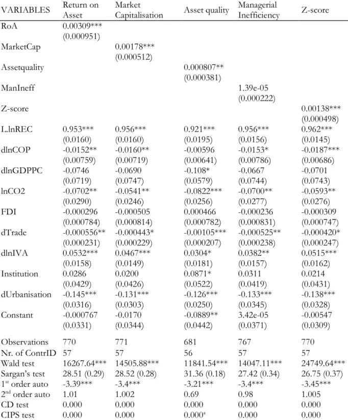
Table 8: Impact of banking sector performance on renewable energy consumption for middle income countries ... 26

Table 9: Impact of banking sector performance on renewable energy consumption for low income countries ... 27

(7)

1 Introduction

Electricity generation from renewable sources has grown rapidly over the recent years (Moomaw et al., 2011). One example is that in 2000, Solar Photovoltaics1_{accounted for 1 TWh of the world's}

electricity generation, a number that had grown to 435 TWh by 2017. Nevertheless, in 2017, the share of modern renewable energy in total final energy consumption had not reached more than 10.3 percent (International Energy Agency, 2018). To accomplish the 2 ℃ goal set out in the Paris agreement, the continuous conversion in energy from fossil fuels to renewable energy sources is crucial. As a way of estimating the effects of global warming, the International Energy Agency has developed three different forward looking scenarios, all of which predicts different effects that the global warming will implicate for the future. To attain what they call the sustainable development scenario, global CO2 emissions will have to peak at around 2020 and be followed by a steep decline.

By 2040, global CO2 emissions will have to be at half of the levels they are at today (International

Energy Agency, 2019).

While there is need for a considerable decrease in CO2 emissions, the global energy demand is

predicted to continue to grow over the coming years. Despite of the continuous growth in energy supply it is estimated that 650 million people will be without access to energy by 2030 (International Energy agency, 2018). About 90 percent of this increase is assessed to be driven by developing countries, motivating number seven of the Sustainable Development Goals which is to achieve universal access to modern energy by 2030 (The 2030 Agenda for Sustainable Development, 2015). Renewable energy targets energy security since it can play an important role in reducing a country’s dependence on imported energy products (like oil and gas). Through reduced emissions of greenhouse gases, renewable energy can also play an important role in helping to address climate change issues (Sadorsky, 2009a). The response to this dual problem will however entail large investments in renewable energy technology, investments that requires financing. It is estimated that in order to reach the sustainable development scenario, global annual investments in renewable energy will have to increase by 97 percent compared with the investment levels of today (International Energy Agency, 2018).

1.1 Problem

The cost of renewable energy has decreased during recent years and continues to fall (McCrone et al., 2018). This is true also for the price of energy storage as battery prices have fallen steeply during

1_{Photovoltaics are a method for generating electric power by using solar cells to convert energy from the}

(8)

the past decade (Henbest et al., 2018). A challenge related to renewable energy extraction has to do with securing a stable energy supply when relying on the nature for the generation of energy. Cheap batteries mean that wind and solar will increasingly be able to run when the wind is not blowing and the sun is not shining. According to a report published by BloombergNEF, battery prices has already fallen by 79 percent compared to prices in 2010, with a prediction of a continuous decrease of 67 percent from today’s prices until 2030 (Henbest et al., 2018).

Graph 1: Renewable energy consumption2_{as a share of total final energy consumption over time}

Source: World Bank, 2019

At the same time as prices in both renewable energy and storage has fallen, oil prices peaked in 2018 compared to the past four years (International Energy agency, 2018). This trend together with reforms and subsidies to promote energy generation from renewable sources are important mechanisms for investments in renewable energy to increase. Policy and other support mechanisms still play an important role in underpinning returns and limiting risks for project developers, indirectly bolstering the availability of finance that is required for investments in renewable energy technology (McCrone et al., 2018). The fact is, that the rapid worldwide expansion of renewable energy has largely been driven by support policies from governments or multilateral institutions. Typically, these aim to address market failures in an effort to promote the uptake of renewable

2_{Renewable energy includes hydro, biomass, wind, solar, liquid biofuels, biogas, geothermal, marine and}

(9)

energy while achieving a number of other objectives, including energy diversification, the development of a local industry and job creation (Lucas et al., 2013).

With the falling prices in renewable technology and storage, one can wonder why there is still such a need of large government interventions for investments in renewable energy to take off. A lower renewable energy price compared to the price of traditional energy sources should be expected to lead to a higher share of energy consumption coming from renewable sources. Graph 1 show that this increase is globally occurring at a very slow pace. Only for low income countries can the average share of renewable energy consumption be said to have made a noticeable increase since 1990. These very modest trends can be explained by the high growth in energy demand over the same period (International Energy agency, 2018). It brings perspective to the proportion of efforts needed to meet the increased demand while lowering CO2 emissions. As can be viewed in Graph

1, low income countries in general have a substantially larger share of renewable energy consumption in relation to total energy consumption than high- and medium income countries. Since 2015, developing countries also exceeds the rest of the world regarding energy investments. Most of this is due to the wide expansion of solar power on the African continent (McCrone et al., 2018).

Substantial research has been made to understand the determinants of energy consumption with a recently increasing focus on the topics of renewable energy consumption and CO2 emissions

(Tamazian et al., 2009; Sadorsky, 2009a, 2009b; Menyah and Wolde-Rufael, 2010; Apergis and Payne, 2010; Menegaki, 2011; Destek and Aslan, 2017). Most commonly have the relationships between energy demand and growth or energy demand and financial development been studied. Islam et al. (2013) find that economic growth increases the demand for energy and that financial development leads to increased energy consumption in the long run. Similarly, Komal and Abbas (2015) and Shahbaz and Lean (2012) find long-run positive effects of financial development and economic growth increases energy consumption.

From a policy standpoint, research has showed that the consumption of renewable energy is a rather complex topic. In an attempt to estimate the effect of renewable energy consumption on economic growth, Bhattacharya et al. (2016) reaches a heterogeneous result with substantial differences in effects across countries. Few articles have looked into the effect that financial development has on consumption of renewable energy. Paramati et al. (2016) find that both foreign direct investment inflows and stock market development are promoting drivers for the generation and use of clean energy in 20 emerging markets over the period 1991-2012. Complementary, Tamazian et al. (2009) show that financial development and especially capital market and banking sector development decreases the environmental degradation by lowering CO2 emissions.

(10)

Financial development can be measured in a number of ways and little attention has been given to the specific role of the bank sector for renewable energy consumption. That a well-performing banking sector has an effect on the use of energy is confirmed in a study by Amuakwa-Mensah et al. (2018). In their article, they look into the relationship between banking performance variables and energy efficiency for 43 sub-Saharan African countries. They find significant results which show that improved banking performance foster energy efficiency. These findings are interesting when going forward with this thesis. If a well-functioning bank sector can foster more efficient energy use, it is likely that the same variables are also determinants when it comes to renewable energy consumption as a share of total final energy consumption.

1.2 Aim and delimitations

Due to the challenges faced by the world to both achieve universal energy access and to lower CO2

emissions, it is important to further investigate the relationship between financial development, and specifically the bank sector, and renewable energy consumption. The transition from generating energy through fossil fuels to renewable energy sources will demand a massive increase in investments directed towards production and storage of renewable energy. It is therefore likely that well-functioning capital markets and a high performing banking sector will stimulate renewable energy consumption. This thesis aims to contribute to the existing literature on financial development and renewable energy by estimating the effect of banking sector performance on renewable energy consumption. For that purpose, a bank-based dataset by Andrianova et al. (2015) will be used. The dataset contains data for 124 countries available for the years 1998-2012. After considering the whole sample, a subgroup analysis will be carried out based on income groupings. This will recognise differences in variable effects between the groups. Several indicators are used to measure banking performance. These are return on asset, market capitalisation, asset quality, managerial inefficiency and Z-score. Z-score measures the level of financial stability. To estimate the effect of banking performance on renewable energy consumption, the two-step system generalised method of moments (sys-GMM) technique is used. The sys-GMM technique deals with problems of simultaneity bias/endogeneity and serial correlation problems. Pesaran’s (2004) section dependence test together with unit root tests are performed. For variables that show cross-sectional dependence, the Pesaran's (2007) cross-cross-sectional augmented panel unit root test (CIPS) is performed. This test accounts for sectional dependence. For the variables that are cross-sectional independent (renewable energy consumption and financial solidity), the augmented Dickey fuller and Phillip-Perron tests are used as unit root tests.

(11)

This study will contribute to the research on the nexus of financial development and renewable energy consumption which has been given little attention in relation to the importance of the topic, if wanting to meet the future energy demand and at the same time lowering CO2 emissions. To fill

the gap in the literature this thesis will use banking sector indicators to establish the effect of the banking sectors performance on renewable energy consumption. As banks are the institutions through which the majority of credit is lent, it is of large interest to analyse the role that they play in the determination of renewable energy consumption. This thesis will be the first study to estimate this relationship as no one previously has looked at the specific role that the banks play in the consumption decision between energy from traditional or renewable sources. Findings suggest that interventions to improve the banking sector and strengthen credit markets will stimulate increases in renewable energy consumption as a share of total energy consumption globally as well as for the three income categories. By using a large sample and dividing the countries into groups by income level, the thesis is also able to point at interesting differences between the groups which can give important policy guidance when attempting to increase renewable energy consumption.

1.3 Structure of the report

The continuation of this thesis is structured as follows. Section 2 provides an overview of the existing literature on the dynamics of renewable energy consumption and financial development. The methodology is presented in section 3 and in section 4, the data and variables are described and tested. Section 5 presents and discusses the empirical findings. Finally, section 6 presents conclusions and suggestions for further studies within the research field.

(12)

2 Literature review

There has been little written on the effect of improved banking performance on renewable energy consumption. To give an overview of the existing research within the field, this section outlines the literature that forms the base on which this thesis is built on.

Kraft and Kraft (1978) found in a pioneering article that growth caused a growing energy demand in the United States between 1947-1974. Since then, the determinants of energy demand have been scrutinised, leading to a large pool of research both on the economic growth and energy consumption nexus (Akinlo, 2008; Bartleet and Gounder, 2010; Ozturk et al., 2010; Arouri et al., 2012; Karanfil and Li, 2015; Bhattacharya et al., 2016) and later on the nexus of financial development and energy consumption (Sadorsky, 2010; Shahbaz and Lean, 2012; Islam et al., 2013; Komal and Abbas, 2015; Kakar, 2016).

On the relationship of growth and energy consumption, the differentiated results within the field has led to the development of four hypotheses (Payne, 2010). These are the growth-, conservation-, feedback- and neutrality hypothesis. The growth hypothesis indicates a unidirectional causality from energy consumption to economic growth whereas the conservation hypothesis indicates the opposite causality that goes from economic growth to energy consumption. The feedback hypothesis is supported if there is bidirectional causality between energy consumption and economic growth and the neutrality hypothesis implies that there is no causal relationship between energy consumption and economic growth (Destek and Aslan, 2017).

Karanfil (2009) elaborates on the determinants of energy consumption stating that the causality between economic growth and energy consumption cannot be justified just by a simple bivariate model. Instead he suggests that one of the financial variables domestic credit to private sector, stock market capitalisation or liquid liabilities should be put into the model as well as exchange rate and interest rate, which could have an effect on energy consumption through energy prices. This conclusion by Karanfil (2009) has inspired researchers to study the link between financial development and energy consumption, something that has led to the formation of two separate hypotheses on what statutes the relationship.

The first of these two hypotheses is that financial development decreases energy consumption. This builds on the assumption that a well-established financial system increases the efficiency of the economy which leads to the usage of resources being more productive. It is therefore assumed that through efficiency gains, financial development can lead to a reduction in energy consumption (Shahbaz and Lean, 2012; Islam et al., 2013; Kakar, 2016). The second hypothesis states the contrary, that financial development increases energy consumption. This is based on the notion

(13)

that a well-functioning financial sector eases the financing process for consumers by lowering the borrowing cost (Karanfil, 2009; Sadorsky, 2011). Consumers will then borrow to invest in energy-intensive products.

When distinguishing renewable energy consumption from energy consumption as a whole, the majority of studies have been investigating the relationship between economic growth and renewable energy consumption (Sadorsky, 2009b; Apergis and Payne, 2010; Menegaki, 2011; Bölük and Mert, 2015; Bhattacharya et al., 2016; Adewuyi and Awodumi, 2017). Sadorsky (2009b) find that increases in real per capita income have a positive and statistically significant impact on per capita renewable energy consumption. Apergis and Payne (2010) find indications for a bidirectional causality between renewable energy consumption and economic growth in both the short- and long-run. This conclusion is supported by Bhattacharya et al. (2016) but dismissed by Menegaki (2011) as she does not find support for a statistically significant relationship between growth and renewable energy consumption when looking specifically at 27 European countries.

Attention has also been payed to other determinants of renewable and non-renewable energy consumption. Bartleet and Gounder (2010) and Shahbaz and Lean (2012) find a co-integration relationship between energy consumption, economic growth and variables such as employment, industrialisation and urbanisation. In the long run Shahbaz and Lean (2012) find that both industrialisation and urbanisation increase energy consumption. Sadorsky (2009a) looks at the effect of CO2 emissions and find it to be an important driver of renewable energy consumption.

On the contrary, Mehrara et al. (2015) reaches the conclusion that CO2 emission have a negative

significant effect on renewable energy consumption for middle eastern countries part of the Economic Cooperation Organization. Aside from CO2 emissions, Mehrara et al. (2015) finds that

political instability and violence, government effectiveness, urban population (% of total) and human capital (school enrolment) are the most robust drivers of renewable energy consumption for the countries within the Economic Cooperation Organization. This is something that Sadorsky (2009a) fail to consider and which can lead to the question if his estimations are biased suffering from endogeneity problems.

In another study on determinants of renewable energy, Omri and Nguyen (2014) applies the same approach as will follow in this thesis by dividing their sample into three income groups when determining which variables that have an effect on renewable energy consumption. They look specifically at variables per capita GDP, oil prices, trade openness and CO2 emissions, all of which

will also be included in this thesis. Conclusions from their study show that i) the impact of environmental degradation (CO2 emissions) is statistically significant across all panels, ii) oil prices

(14)

capita GDP significantly affect the renewable energy consumption only in the high- and low-income countries and iv) that changes in the trade openness variable have a statistically significant effect on the renewable energy consumption for all the panels with the exception of the high-income panel (Omri and Nguyen, 2014). That oil prices have a negative effect on renewable energy consumption would mean that crude oil and renewable energy have a complementary relationship rather than a supplementary relationship.

Very few studies have recognised the role of financial development related to renewable energy consumption. In one study, Paramati et al. (2016) estimates the effect of foreign direct investment and stock market growth on clean energy and concludes that these variables are drivers of both generation and use of clean energy. In a resembling article, Dogan and Seker (2016) estimate that trade and financial development can help countries to adopt and use new environmentally-friendly technologies which will in turn boosts renewable energy consumption. Even though there has not been any substantial research made on how financial variables affect renewable energy consumption, researchers have drawn conclusions which would suggest that the commercial banks and the banking sector has a vital part to play if aiming at increasing renewable energy consumption. Omri and Nguyen (2014), when discussing policy implications of their study, suggests that a decreased cost of credit would help stimulate renewable energy consumption. This would support the hypothesis of this thesis, that a well-performing bank sector increases renewable energy consumption.

Banking sector performance has previously been studied in relation to energy efficiency in the context of sub-Saharan Africa, where it has been proved to have a positive effect on energy efficiency (Amuakwa-Mensah et al., 2018). As suggested in their study, this thesis applies the neoclassical model used by Amuakwa-Mensah et al. (2018) to further examine the nexus between renewable energy consumption and financial development, specifically focusing on the role of the bank sector.

(15)

3 Method

The theoretical framework in this thesis assumes a neoclassical economic model where firms maximises their profits, following the work of Adom and Mensah (2016) and Amuakwa-Mensah et al. (2018).

3.1 Theoretical framework

Each firm seaks to maximise their profit by choosing the optimal level of input, which in this case is energy input. The model assumes Cobb-Douglas technology such that each firm maximises profit subject to Cobb-Douglas production technology.

𝑀𝑎𝑥_𝐸,𝑍 → 𝜋 = 𝑃𝑌 − 𝑃_𝑒𝐸 − 𝑍 (1)

Subject to: 𝑌 = 𝐴𝐸𝛼_𝑍𝛽 ₍₂₎

The variables 𝜋, 𝑃, 𝑌, 𝑃𝑒, 𝐸, 𝐴 and 𝑍 are firm’s profit, output price, output, price of energy input,

energy input, total factor productivity and composite input (with a price normalised to one) respectively. 𝛼 and 𝛽 indicate respective share of energy input and composite input in total production. The Lagrangian equation is used to solve the optimisation problem:

ℒ

= 𝑃𝑌 − 𝑃_𝑒𝐸 − 𝑍 + 𝜆(𝑌 − 𝐴𝐸𝛼_𝑍𝛽₎ ₍₃₎

The Lagrangian is differentiated with respect to energy (𝐸), composite input (𝑍) and the Lagrangian multiplier (𝜆). This gives the following first order conditions for the maximisation problem; 𝑑𝐿 𝑑𝐸 = −𝑃𝑒− 𝜆𝛼𝐴𝐸𝛼−1𝑍𝛽= 0 (4) 𝑑𝐿 𝑑𝑍 = −1 − 𝜆𝛽𝐴𝐸 𝛼_𝑍𝛽−1_{= 0} ₍₅₎ 𝑑𝐿 𝑑𝜆= 𝑌 − 𝐴𝐸𝛼𝑍𝛽 = 0 (6)

By solving the first order conditions one gets the optimal demand for energy and composite input required for the firm to achieve optimal profit for a given level of technology. As this thesis is studying the effects of banking performance on renewable energy, it will solely focus on optimal energy input. This is given as:

𝐸 = (𝛼_𝛽) 𝛼𝛽 𝛼𝛽+1₍1 𝑃𝑒) 𝛼𝛽 𝛼𝛽+1₍1 𝐴) 𝛼 𝛼𝛽+1_𝑌_𝛼𝛽+1𝛼 (7) This equation shows that the firm’s optimal demand for energy is inversely proportional to price and technology and increases with output. To include banking performance in the model, total

(16)

factor productivity can be described as a positive exponential function of financial performance (FP), foreign direct investment (FDI), trade openness (TO) and institutional quality (Instit) (Adom and Amuakwa-Mensah, 2016; Amuakwa-Mensah et al., 2018).

𝐴 = 𝑒𝑓(𝛽2𝐹𝑃,𝛽3𝐹𝐷𝐼,𝛽4𝑇𝑂,𝛽5𝐼𝑛𝑠𝑡𝑖𝑡) ₍₈₎

In the expression for energy demand (equation 7), 𝐴 can then be replaced by equation 8 yielding the following expression for energy demand:

𝐸 = (𝛼_𝛽) 𝛼𝛽 𝛼𝛽+1₍1 𝑃𝑒) 𝛼𝛽 𝛼𝛽+1₍ 1 𝑒𝛽2𝐹𝑃+𝛽3𝐹𝐷𝐼+𝛽4𝑇𝑂+𝛽5𝐼𝑛𝑠𝑡𝑖𝑡)) 𝛼 𝛼𝛽+1_𝑌_𝛼𝛽+1𝛼 (9) By taking the natural logaritm on both sides we get:

ln 𝐸 =_𝛼𝛽+1𝛼𝛽 ln (𝛼_𝛽) −_𝛼𝛽+1𝛼𝛽 ln 𝑃_𝑒−_𝛼𝛽+1𝛼 (𝛽₂𝐹𝑃 + 𝛽₃𝐹𝐷𝐼 + 𝛽₄𝑇𝑂 + 𝛽₅𝐼𝑛𝑠𝑡𝑖𝑡) +_𝛼𝛽+1𝛼 ln 𝑌 (10) Equation 10 can then, for simplicity, be written as:

ln 𝐸 = 𝛾0− 𝛾1ln 𝑃𝑒− 𝛾2𝐹𝑃 − 𝛾3𝐹𝐷𝐼 − 𝛾4𝑇𝑂 − 𝛾5𝐼𝑛𝑠𝑡𝑖𝑡 + 𝛾6ln 𝑌 (11)

Here 𝛾0 is the constant term on the right hand side of the equation and 𝛾1, 𝛾2, 𝛾3, 𝛾4, 𝛾5 and

𝛾₆ are the respective coefficients of cruide oil price, financial performance, foreign direct investment, trade openness, institutional quality and income.

3.2 Estimation methodology

Since it is the effect of banking performance on renewable energy consumption that is the subject of interest for this thesis, renewable energy will henceforth be used as the source of energy input. This follows by the assumption that energy demand is determined by equation 11, regardless of the source of energy input. Renewable energy is measured as the share of total final energy consumption that comes from renewable sources. This includes renewable energy consumption of all technologies: hydro, biomass, wind, solar, liquid biofuels, biogas, geothermal, marine and renewable wastes (International Energy Agency, 2018). Following equation 11, the empirical model is expressed as:

ln 𝑅𝐸𝑖𝑡 = 𝛾0+ 𝜆 ln 𝑅𝐸𝑖𝑡−1− 𝛾1ln 𝑃𝑒𝑡− 𝛾2𝐹𝑃𝑖𝑡− 𝛾3𝐹𝐷𝐼𝑖𝑡 − 𝛾4𝑇𝑂𝑖𝑡 − 𝛾5𝐼𝑛𝑠𝑡𝑖𝑡𝑖𝑡

+𝛾₆ln 𝑌_𝑖𝑡+ 𝜸𝑿_𝒊𝒕+ 𝜂_𝑖 + 𝑣_𝑡+ 𝜀_𝑖𝑡 (12)

Each 𝛾 takes on the previously described definitions whereas 𝜆 is the coefficient of the lagged dependent variable. 𝜸𝑿𝒊𝒕 symbolises the coefficient and vector of other control variables that can

(17)

trade and institutional quality. Other control variables that will be included in the econometric estimations are urbanisation, industry (value added), industrial growth and carbon oxide (CO2)

emissions. These are taken from the literature studying determinants of both energy consumption as well as renewable energy consumption (Sadorsky, 2009; Aguirre and Ibikunle, 2014; Shahbaz and Lean, 2012). When estimating country level data, it can be difficult to avoid endogeneity problems if only including control variables related to the economic state of a country. As mentioned, it has been proven that governing and institutional indicators show significant effect on a country’s environmental condition (Mehrara et al., 2015). In an attempt to avoid endogeneity and control for these country characteristics, control variables institutional quality and urbanisation (% of total population) will be included in the estimations.

The 𝜂𝑖 and 𝑣𝑡 respectively captures the country and time fixed effects and the error term is denoted

as 𝜀_𝑖𝑡. Bank performance is indicated by the variables return on asset, asset quality, bank capitalisation and managerial inefficiency. The Z-score is used to measure the stability of the financial system (Andrianova et al., 2015). In the following section 4, which covers information about the data used in this study, the variables used in the econometric estimations will be further defined and described.

3.3 Assumptions of the neoclassical economic framework

The neoclassical framework implies that the economy allocates resources most efficiently through markets, assuming that economic agents are rational and have perfect knowledge. In a market, an equilibrium will occur which maximises the benefits to economic agents given the law of diminishing returns, many agents buying and selling, and freedom to enter and leave the market. The basic message of neoclassical economics is that economic efficiency and economic progress are maximised by ensuring that markets work freely and competitively (Nicholson, 2005). For this to work, several assumptions have to be applied. Three assumptions that are central in neoclassical economics are; i) people have rational preferences among outcomes, ii) individuals maximise utility and firms maximise profits and iii) people and firms act independently on the basis of full and relevant information (Weintraub, 2002).

3.4 Econometric method

For our econometric estimations, equation 12 will be estimated by using the two-stage system general method of moments (system-GMM) technique. The system-GMM is useful since it allows for the lagged level of the renewable energy consumption as equation 12 exhibits. The lagged version of the dependent variable (renewable energy consumption) is included to capture the

(18)

persistence of renewable energy consumption. It is highly reasonable to expect that if a country had a high level of renewable energy consumption in one year, it would probably remain at a high level also the following year. To not include the lagged dependent variable would probably lead to a high correlation between the dependent variable and the error term, causing biased estimations. However, if the estimation were to be done using an ordinary least squares estimation, the included lagged dependent variable could lead to inconsistent estimates. That is due to the problems of autocorrelation of the residuals and endogeneity of the regressors. The system-GMM method uses a set of internal instrumental variables to solve the endogeneity problem of the regressors. There are two types of GMM estimators (difference and system) and they could both be alternatively considered in their one-step and two-step versions. Arellano and Bond (1991) initially suggested the one-step difference-GMM which introduced the set of internal instruments to solve the described inconsistencies of the ordinary least squares estimation. The set of instruments of the difference-GMM estimator includes all the available lags in difference of the endogenous variables and the strictly exogenous regressors. This method was however later pointed out to be suffering from bias, showing imprecise estimates (Blundell and Bond, 1998). Blundell and Bond (1998) instead introduced the system-GMM estimator. The system-GMM estimator, which is used in this study, includes not only the previous instruments of the difference-GMM but also the lagged values of the dependent variable. This solves the bias and imprecision by first assuming independent and homoscedastic error terms and then using the first-step residuals to construct consistent variance and covariance matrices in the second stage. This method can however, in finite sample cases, lead to a downward bias for the standard errors (Amuakwa-Mensah et al., 2018). The system-GMM is advantageous in that it helps solve the endogeneity problem arising from the potential correlation between the independent variable and the error term in dynamic panel data models. It is also favourable to use over the difference-GMM when working with unbalanced panel data such as in this thesis (Çoban and Topcu, 2013).

To avoid the problem of a downward bias in standard errors, this thesis will minimise the number of lags and then use the Sargan test to check instrumental validity. To test for serial correlation, I hypothesised serial correlation at first-order but no serial-correlation at second order. Each model will also have a cross-sectional dependence and stationary test of the residual term carried out. When the residual term from the model is stationary, it provides an evidence of the model goodness of fit (Sadorsky, 2013).

(19)

4 Data and tests

As defined in the previous section, the dependent variable in the econometric estimations will be renewable energy consumption. To estimate the effect of banking performance on renewable energy consumption, five banking sector variables will be used as the independent variables of interest. Each estimation will control for a lagged version of renewable energy consumption, crude oil price, per capita GDP, CO2 emissions, foreign direct investment, trade openness, industrial

value added, institutional quality and urbanisation. This section will further describe the dataset and variables used. It will also include relevant tests which are important to perform before continuing to the estimations.

4.1 Data and variable description

This study uses panel data covering 124 countries over the period 1998-2012. Data on banking performance are sourced from the International Database on Financial Fragility created by Andrianova et al. (2015). The International Database on Financial Fragility uses bank data from five types of financial institutions; commercial banks, co-operative banks, Islamic banks, real estate and mortgage banks. Data is collected from 23 287 banks where commercial banks accounts for about two thirds of the banking frequency (Andrianova et al., 2015). In this thesis, I use the five variables related to banks performance from the dataset by Andrianova et al. (2015) to estimate the relationship between the performance of the banks and consumption of renewable energy. These are return on asset, market capitalisation (bank size), Z-score (financial stability), asset quality (non-performing loans) and managerial inefficiency (cost to revenue ratio). Crude oil prices are from the BP Statistical Review of World Energy. Data on renewable energy and other macroeconomic variables are collected from the World Bank’s World Development Indicator (WDI), whereas the institutional variable proxy is sourced from Polity IV Project. The Polity IV Project is developed to monitor regime change and studying the effects of regime authority (Marshall, 2018). Some variables in the data, especially asset quality, institution and industry, contain missing values making the panel unbalanced. To make the panel as balanced as required to perform the estimations, some countries have been dropt from the sample.3_{Because of the large number of observation, this is}

not expected to have an impact on the estimated results.

3_{Seychelles, Russian Federation, Cote d'Ivoire, Hong Kong, Sao Tome and Principe, Djibouti, Angola,}

(20)

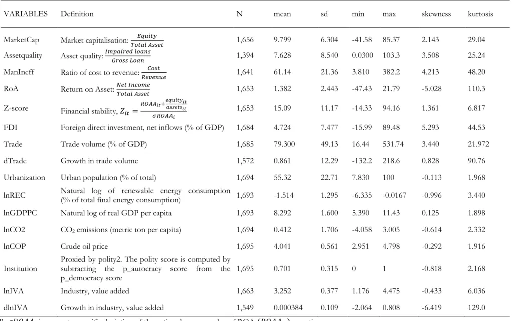
Table 1: Description of variables and statistics

VARIABLES Definition N mean sd min max skewness kurtosis

MarketCap Market capitalisation: _{𝑇𝑜𝑡𝑎𝑙 𝐴𝑠𝑠𝑒𝑡}𝐸𝑞𝑢𝑖𝑡𝑦 1,656 9.799 6.304 -41.58 85.37 2.143 29.04

Assetquality Asset quality: 𝐼𝑚𝑝𝑎𝑖𝑟𝑒𝑑 𝑙𝑜𝑎𝑛𝑠_{𝐺𝑟𝑜𝑠𝑠 𝐿𝑜𝑎𝑛} 1,394 7.628 8.540 0.0300 103.3 3.508 25.24

ManIneff Ratio of cost to revenue: _{𝑅𝑒𝑣𝑒𝑛𝑢𝑒}𝐶𝑜𝑠𝑡 1,641 61.14 21.36 3.810 382.2 4.213 48.20

RoA Return on Asset:𝑁𝑒𝑡 𝐼𝑛𝑐𝑜𝑚𝑒_{𝑇𝑜𝑡𝑎𝑙 𝐴𝑠𝑠𝑒𝑡} 1,653 1.382 2.443 -47.43 21.79 -5.028 110.3

Z-score _{Financial stability, 𝑍}_𝑖𝑡 ₌𝑅𝑂𝐴𝐴𝑖𝑡+𝑒𝑞𝑢𝑖𝑡𝑦𝑖𝑡_{𝑎𝑠𝑠𝑒𝑡𝑠𝑖𝑡}

𝜎𝑅𝑂𝐴𝐴𝑖

1,653 15.09 11.17 -14.33 94.16 1.361 6.817

FDI Foreign direct investment, net inflows (% of GDP) 1,684 4.724 7.477 -15.99 89.48 5.293 44.53

Trade Trade volume (% of GDP) 1,685 79.300 49.13 16.44 531.74 3.440 21.972

dTrade Growth in trade volume 1,572 0.861 12.29 -132.2 218.6 0.828 90.76

Urbanization Urban population (% of total) 1,694 55.32 22.71 7.830 100 -0.113 1.968

lnREC Natural log of renewable energy consumption _{(% of total final energy consumption)} 1,693 -1.514 1.295 -6.335 -0.0167 -0.996 3.440

lnGDPPC Natural log of real GDP per capita 1,693 8.292 1.600 5.390 11.43 0.125 1.898

lnCO2 CO2 emissions (metric ton per capita) 1,694 0.412 1.706 -4.058 3.005 -0.614 2.332

lnCOP Crude oil price 1,695 4.041 0.561 2.951 4.798 -0.292 1.916

Institution Proxied by polity2. The polity score is computed by subtracting the p_autocracy score from the

p_democracy score 1,695 0.701 0.315 0 1 -0.818 2.168

lnIVA Industry, value added 1,663 3.252 0.377 1.176 4.475 -0.433 6.036

dlnIVA Growth in industry, value added 1,549 0.000384 0.109 -2.064 0.808 -6.419 129.0

(21)

Renewable energy consumption is defined as the share of renewable energy in total final energy consumption. Total final energy consumption is in turn derived from energy balances statistics and is equivalent to total final end use consumption excluding non-energy use (World Bank, 2018). Regarding control variables used, Omri and Nguyen (2014) has studied the determinants of renewable energy consumption. They find CO2 emissions to be a significant determinant of

renewable energy consumption both when estimating global effects as well as for high, middle and low income groups. Crude oil price, per capita GDP and trade openness are also shown to have effects on renewable energy consumption but show heterogeneous results across the different income groups. In this thesis, CO2 emissions is expressed as CO2 emissions per capita (metric

tons). GDP serves as a measure of output and GDP figures are in 2011 US dollars. GDP has been divided by total population of each country to get a per capita GDP measure. Urbanisation and industrialisation will be included as control variables as both have been proved to have a significant effect on energy use and CO2 emissions (Sadorsky, 2013; Li and Lin, 2015).

Table 1 defines and presents the descriptive statistics for each variable. The top rows show the five variables that are used to describe banking sector performance. Market capitalisation is defined as the ratio between equity and total asset. The average market capitalisation for banks in the sample is 9.8 with a standard deviation of 6.3. Asset quality is the ratio between impaired loans and gross loans and can also be expressed as share of non-performing loans. It has a mean of 7.63 and a standard deviation of 8.54. Managerial inefficiency is the cost to revenue ratio and it is on average 61.14 with a standard deviation of 21.36. This high value shows that banks in the sample generally are inefficiently managed. A management which deploys its resources efficiently will look to maximise its income and reduce its operating costs. Therefore, a larger ratio implies a lower level of efficiency. Return on asset has a mean of 1.382 and a standard deviation of 2.443. Both asset quality and return on asset suggests a high variability for countries across years since the standard deviation is larger than the mean. Market capitalisation, asset quality and managerial inefficiency are all positively skewed with more in tails than a normal distribution. Return on asset also has larger tails than a normal distribution but is instead negatively skewed. The average Z-score, which measures financial stability, is 15.09 with a standard deviation of 11.17. The higher the Z-score, the more financially sound a country is (Andrianova et al., 2015). The distribution for Z-score is positively skewed with more in tails than a normal distribution.

For the whole sample, the log of the renewable energy consumption variable has a mean of -1.514 with a standard deviation of 1.295. This translates so that the share of renewable energy

(22)

consumption of total final energy consumption has a sample mean of 22 percent.4_Renewable

energy consumption is negatively skewed with a larger tail on the left than a normal distribution. Mean GDP per capita is about 3741 US dollars with a standard deviation of 5 US dollars. CO2

emissions has a mean of about 1.5 metric tons per capita and a standard deviation of 5.5 metric tons per capita. The institution variable measures on a scale from 0 to 1, where 0 indicates strongly autocratic institutions and 1 indicates strongly democratic institutions in a country.5_{The sample}

mean is 0.701 and the standard deviation is 0.315.

The variable foreign direct investment is expressed as percentages of GDP. On average, net foreign direct investment inflows are about 4.7 percent of GDP with a standard deviation of about 7.5 percent of GDP. Trade is expressed both as a percentage of GDP and in its growth form since it is the latter that will be used in the estimations. The average trade volume is 79.3 percent of GDP with a standard deviation of 49 percent. The growth form of trade has a mean of 0.86 percent and the standard deviation is 12.3 percent. Urbanisation is expressed as a percentage of total population and has a sample mean of 55 percent. The standard deviation is about 23 percent. Foreign direct investment and trade are positively skewed with larger tails than a normal distribution, while urbanisation is close of being normally distributed.

4.2 Cross-sectional dependence, unit root test and correlation matrix

Before preforming the empirical estimations, some tests are performed to ensure the reliance and consistence of the results presented in section 5 of this study. A cross-sectional dependence (CD) test is used to determine whether or not the variables of interest correlate across countries. To test for unit root, a unit root test is performed using three different methods (augmented Dick Fuller, Phillip-Perron and Pesaran’s CIPS test). When determining the correlation between pairs of variables, a correlation matrix is presented and evaluated.

4.2.1 Testing for the entire sample

To determine if the variables are correlated across countries the Pesaran’s (2004) cross-section dependence test is used. Researchers have pointed out that empirical variables are more likely to show cross-sectional dependence than to live up to the assumption of cross-sectional independence (Banerjee et al., 2004; Pesaran, 2015). De Hoyos and Sarafidis (2006) highlights the need of testing for cross-section dependence if T is small and N is large. That description fits the data used in this thesis where T=15 and N=113 after excluding countries exhibiting large counts

4_{Taking the log transformation of the figure -1.514 in Table 1.}

5_{Polity2 ranges from -10 to 10 in the Polity IV Project dataset. When used in this thesis it is transformed}

(23)

of missing values. Pesaran’s (2004) cross-sectional dependence test is used since it is valid under a wide class of panel data models (Sarafidis and Wansbeek, 2012).

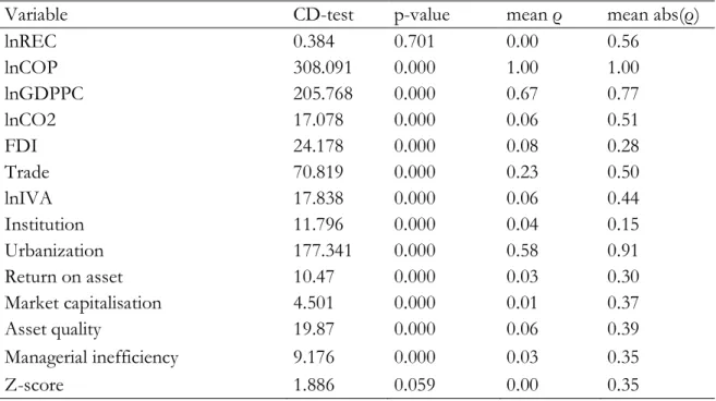
Table 2: Cross-section dependence test

Variable CD-test p-value mean ρ mean abs(ρ)

lnREC 0.384 0.701 0.00 0.56 lnCOP 308.091 0.000 1.00 1.00 lnGDPPC 205.768 0.000 0.67 0.77 lnCO2 17.078 0.000 0.06 0.51 FDI 24.178 0.000 0.08 0.28 Trade 70.819 0.000 0.23 0.50 lnIVA 17.838 0.000 0.06 0.44 Institution 11.796 0.000 0.04 0.15 Urbanization 177.341 0.000 0.58 0.91 Return on asset 10.47 0.000 0.03 0.30 Market capitalisation 4.501 0.000 0.01 0.37 Asset quality 19.87 0.000 0.06 0.39 Managerial inefficiency 9.176 0.000 0.03 0.35 Z-score 1.886 0.059 0.00 0.35

Notes: Under the null hypothesis of cross-section independence, CD ~ N(0,1) P-values close to zero indicate data are correlated across panel groups.

In Table 2, the result from the cross-section dependence test over the entire sample is displayed. In line with the projection by Banerjee et al. (2004) and Pesaran (2015) above, all variables except the dependent variable of renewable energy consumption show results rejecting the null hypothesis of cross-sectional independence. The Z-score variable show a weak tendency of cross-sectional independence where the null hypothesis only is rejected at a 10 percent significance level. The other variables strongly reject the null hypothesis of cross-sectional independence at the 1 percent significance level. The dependent variable of renewable energy consumption is the only variable being cross-sectional independent.

The unit root test is testing whether a variable is stationary at level or not. The variables need to be stationary such that mean, variance, autocorrelation, etc. all are constant over time before using the variables in econometric estimations. For the cross-sectional independent variables, the panel augmented Dick Fuller and Phillip-Perron tests are used to perform the unit root test. These tests are widely used since they account for individual unit root process and as such deals with heterogeneity. Both tests are used since even if the augmented Dick Fuller test show that variables are stationary, the Phillip-Perron test (which has more power) show that some variables only become stationary after first difference. For variables that are cross-sectional dependent, neither of these tests can be relied upon since they assume cross-sectional independence. Therefore, for the

(24)

variables showing cross-sectional dependence, the Pesaran (2007) cross-sectional augmented panel unit root test (CIPS) is used which accounts for cross-sectional dependence.

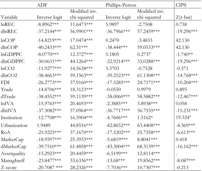
Table 3: Unit root test

ADF Phillips-Perron CIPS

Variable Inverse logit Modified inv. chi-squared Inverse logit Modified inv. chi-squared Z(t-bar)

lnREC -8.8962*** 11.6473*** 5.9897 -2.7508 0.738 dlnREC -37.2144*** 56.9901*** -36.7966*** 57.2459*** -19.296*** lnCOP -14.8219*** 17.0474*** 0.2470 -3.4833 42.130 dlnCOP -40.2433*** 62.31*** -38.444*** 59.0533*** 42.130 lnGDPPC -8.0770*** 12.3727*** 5.1805 0.2737 -1.740** dlnGDPPC -30.0631*** 44.1264*** -22.9214*** 33.0288*** -19.296*** lnCO2 -11.9277*** 14.5638*** 3.3703 -0.7528 -0.571 dlnCO2 -38.4663*** 59.1563*** -39.2523*** 61.1308*** -14.768*** FDI -26.2773*** 37.9160*** -17.5285*** 24.7171*** -10.204*** Trade -14.8706*** 18.3123*** -0.0550 0.9979 0.895 dTrade -38.4552*** 59.1139*** -38.0060*** 58.5882*** -12.467*** lnIVA -15.9765*** 20.4693*** -2.3885*** 3.8938*** 0.058 dlnIVA -37.3082*** 57.0964*** -36.7717*** 56.7535*** -15.231*** Institution -12.7708*** 16.5904*** -4.7606*** 1.5162* 19.324a Urbanization 1.9489 44.8516*** -42.8652*** 63.4408*** -4.369*** RoA -25.9225*** 37.1670*** -17.5202*** 25.7558*** -6.613*** MarketCap -18.9597*** 25.3933*** -5.6819*** 8.8041*** 0.418 dMarketCap -39.7510*** 61.4858*** -43.3004*** 68.3139*** -16.162*** Assetquality -15.2923*** 20.4459*** -6.5199*** 12.8114*** . ManagIneff -23.8477*** 33.6336*** -13.68*** 19.8562*** -8.087*** Z-score -20.7087 *** 28.2326*** -7.7036*** 10.7307*** -0.213

*** p<0.01, ** p<0.05, * p<0.1. a indicates that test wasn’t stationary at level nor at first difference.

The three columns in Table 3 presents the augmented Dick Fuller and Phillip-Perron as well as the Pesaran (2007) cross-sectional augmented panel unit root test (CIPS). Renewable energy consumption and the Z-score were the variables that, according to the above cross-section dependence test, showed cross-sectional independence. For these two variables, I regard the augmented Dick Fuller and Phillip-Perron as the indicator of unit root. From Table 3 we get that Z-score is stationary at level, while renewable energy consumption is stationary at first difference. The rest of the variables are evaluated based on the CIPS-test. It shows that foreign direct investment, urbanisation, return on asset and managerial inefficiency are stationary at level. Crude oil price, per capita GDP, CO2 emissions, trade, industry value added and market capitalisation are

(25)

not stationary at level and needs to be transformed into growth form before being put into the estimation model.6

For the variables used in the econometric estimation, a correlation matrix is presented in Table A2 in the appendix. It shows no high correlation between the pair of variables, indicating that the presence of multicollinearity in the econometric estimations is low.

4.2.2 Testing data for each income group.

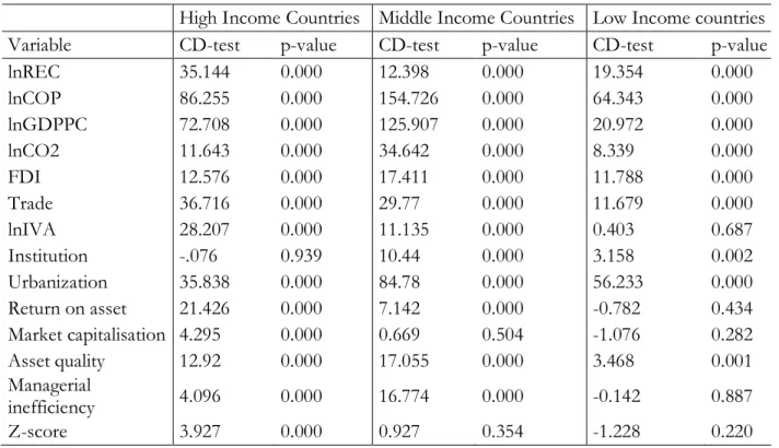
Table 4: Cross-section dependence test per income group

High Income Countries Middle Income Countries Low Income countries

Variable CD-test p-value CD-test p-value CD-test p-value

lnREC 35.144 0.000 12.398 0.000 19.354 0.000 lnCOP 86.255 0.000 154.726 0.000 64.343 0.000 lnGDPPC 72.708 0.000 125.907 0.000 20.972 0.000 lnCO2 11.643 0.000 34.642 0.000 8.339 0.000 FDI 12.576 0.000 17.411 0.000 11.788 0.000 Trade 36.716 0.000 29.77 0.000 11.679 0.000 lnIVA 28.207 0.000 11.135 0.000 0.403 0.687 Institution -.076 0.939 10.44 0.000 3.158 0.002 Urbanization 35.838 0.000 84.78 0.000 56.233 0.000 Return on asset 21.426 0.000 7.142 0.000 -0.782 0.434 Market capitalisation 4.295 0.000 0.669 0.504 -1.076 0.282 Asset quality 12.92 0.000 17.055 0.000 3.468 0.001 Managerial inefficiency 4.096 0.000 16.774 0.000 -0.142 0.887 Z-score 3.927 0.000 0.927 0.354 -1.228 0.220

Notes: Under the null hypothesis of cross-section independence, CD ~ N(0,1) P-values close to zero indicate data are correlated across panel groups.

Since part of the coming analysis is to estimate the different effects for the three income categories, Table 4 presents the results from Pesaran’s (2004) cross-sectional independence test for the different income groups. This shows some interesting findings in terms of which variables that are cross-sectional independent in each income group. For high income countries, all variables except the institution variable are cross-sectional dependent. The column for middle income countries prove that market capitalisation and Z-score are cross-sectional independent whilst the test for the other variables are rejecting the null hypothesis. For the low income counties, all banking performance variables (expect asset quality) are cross-sectional independent along with the industry variable. This result is consistent with previous work focusing on sub-Saharan Africa, being a

6_{The CIPS(Z(t-bar)) unit root test could not estimate for asset quality since data on the variable didn’t}

(26)

region that mainly consists of countries that, in this dataset, is defined as low income countries (Amuakwa-Mensah et al., 2018).

As for the entire sample, the result from the cross-section dependence test for the different income groups in Table 4 gives guidance for which unit root test that is to be relied upon for the different variables. Tables A3, A5 and A7 in the appendix present the results from the unit root tests for each income group. They provide us with some differences regarding which variables are stationary for which income groups. Table A3 indicate that for high income countries the growth form should be used for the variables crude oil price, CO2 emissions, per capita GDP, industry value added,

trade, market capitalisation and Z-score. For estimations covering middle income countries, Table A5 suggests that the growth form be used on variables crude oil price, per capita GDP, industry value added, trade and urbanisation. Table A7 indicate that for low income countries, the variables transformed into growth form before added into the estimations be crude oil price, CO2 emissions,

per capita GDP, industry value added and trade.

For each income group, a correlation matrix is presented in the appendix. Table A4, A6 and A8 describes the correlation coefficients between pairs of variables for high-, middle- and low income countries respectively. The correlation tests show no high correlation between the dependent variable and the independent variables of interest for any panel. By this, it can be assumed that the presence of multicollinearity in the econometric estimations is low.

(27)

5 Empirical findings and discussion

In order to analyse how banking sector performance effects renewable energy consumption, estimations will be carried out on a sample including all the countries in the dataset. Additionally, a subsample analysis will be performed for the three income groups of high-, middle- and low income countries. This will be followed by a discussion on the implications of the results found.

5.1 Impacts of banking sector performance on the global panel

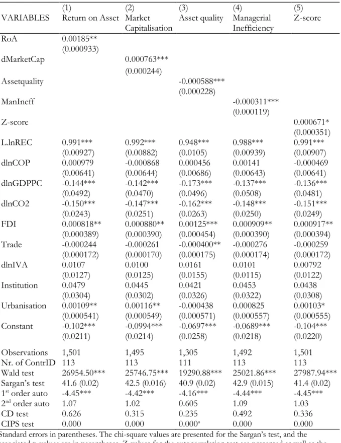
The columns (1) to (5) in Table 5 show the impact of each banking sector variable on the dependent variable renewable energy consumption. Each estimation is done using the system-GMM and the banking performance variables are included step-wise and estimated separately in each column. For the global panel, Table 5 show that all banking performance have a significant effect on the dependent variable, the share of renewable energy consumption. Return on asset and market capitalisation can be seen to increase the share of energy, in relation to total energy consumption, consumed from renewable sources. Asset quality, which is defined as the share of non-performing loans, has a significant negative effect on renewable energy consumption. This implies that a higher share of non-performing loans decreases renewable energy consumption. The same is shown for the variable managerial inefficiency which does also exhibit significant negative effect on the dependent variable. A mismanaged banking sector can thus be said to negatively affect renewable energy consumption. Z-score is viewed to have a positive effect on renewable energy consumption implying that a more stable financial environment is fostering increases in renewable energy consumption.

The coefficients presented in Table 5 suggests that return on asset has the largest separate impact on the share of energy consumed from renewable sources. An increase by one unit in return on asset will significantly increase the renewable energy consumption as a share of total energy consumption by 0.19 percentage points. Since market capitalisation was stationary at first difference for the global panel, the growth form of the variable is used in the estimations that includes all countries. The estimation suggests that a one-unit increase in the growth of market capitalisation increases renewable energy consumption by about 0.08 percentage points. Asset quality (indicating the share of total loans that is non-performing) and managerial inefficiency (cost to revenue ratio) are respectively decreasing the share of renewable energy consumption by about 0.06 and 0.03 percentage points each.7_{A marginal increase in Z-score increases energy consumed}

from renewable sources by about 0.007 percentage points. That would suggest that financial

(28)

stability has an increasing effect on renewable energy consumption in relation to energy consumption from other sources.

Table 5: Impact of banking sector performance on renewable energy consumption

(1) (2) (3) (4) (5)

VARIABLES Return on Asset Market

Capitalisation Asset quality Managerial Inefficiency Z-score

RoA 0.00185** (0.000933) dMarketCap 0.000763*** (0.000244) Assetquality -0.000588*** (0.000228) ManIneff -0.000311*** (0.000119) Z-score 0.000671* (0.000351) L.lnREC 0.991*** 0.992*** 0.948*** 0.988*** 0.991*** (0.00927) (0.00882) (0.0105) (0.00939) (0.00907) dlnCOP 0.000979 -0.000868 0.000456 0.00141 -0.000469 (0.00641) (0.00644) (0.00686) (0.00643) (0.00641) dlnGDPPC -0.144*** -0.142*** -0.173*** -0.137*** -0.136*** (0.0492) (0.0470) (0.0496) (0.0508) (0.0481) dlnCO2 -0.150*** -0.147*** -0.162*** -0.148*** -0.151*** (0.0243) (0.0251) (0.0263) (0.0250) (0.0249) FDI 0.000818** 0.000880** 0.00125*** 0.000909** 0.000917** (0.000389) (0.000390) (0.000454) (0.000390) (0.000394) Trade -0.000244 -0.000261 -0.000400** -0.000276 -0.000259 (0.000172) (0.000170) (0.000175) (0.000174) (0.000172) dlnIVA 0.0107 0.0100 0.0161 0.0101 0.00792 (0.0127) (0.0125) (0.0155) (0.0115) (0.0122) Institution 0.0479 0.0445 0.0421 0.0453 0.0438 (0.0304) (0.0302) (0.0326) (0.0322) (0.0308) Urbanisation 0.00109** 0.00116** -0.000438 0.000825 0.00103* (0.000541) (0.000549) (0.000571) (0.000557) (0.000555) Constant -0.102*** -0.0994*** -0.0697*** -0.0689*** -0.104*** (0.0211) (0.0214) (0.0258) (0.0218) (0.0220) Observations 1,501 1,495 1,305 1,492 1,501 Nr. of ContrID 113 113 111 113 113 Wald test 26954.50*** 25746.75*** 19290.88*** 25021.86*** 27987.94*** Sargan’s test 41.6 (0.02) 42.5 (0.016) 40.9 (0.02) 42.9 (0.015) 41.4 (0.02) 1st_{order auto} _-4.45*** _-4.42*** _-4.16*** _-4.44*** _-4.45*** 2nd_{order auto} _1.07 _1.02 _0.605 _1.09 _1.03 CD test 0.626 0.315 0.235 0.492 0.336 CIPS test 0.000 0.000 0.000a _0.000 _0.000

Standard errors in parentheses. The chi-square values are presented for the Sargan’s test, and the associated p-values are in parentheses. Z-values for the autocorrelation test are presented as well as the chi-square. P-values for the CD and CIPS tests are reported. a indicates instances where the CIPS test could not work in Stata and instead the ADF-test is used.

(29)

The lagged variable for renewable energy consumption show a large positive effect on the dependent variable across all models in the table. This should be of no surprise. If a large share of energy consumed one year comes from renewable sources, it is likely that this will contribute to a high share of energy consumption stemming from renewable sources also the year after.

Table 5 includes a range of tests to determine how reliable the estimated results are. These are the Wald chi-squared test for variable significance, Sargan’s test for testing over-identification and an autocorrelation test. The p-values for the cross-sectional and the CIPS test over the model residuals are also shown in the table. The large coefficients of the Wald chi-squared test tells us that the variables contribute to the model fit and should not be moved from the model (Agresti, 2012). According to the Sargan’s test, our model satisfies the autocorrelation assumptions for all explanatory variables. However, in Table 5, the p-values for the Sargan’s test is rejecting the null at a 5 percent significance level across all models. That indicates that the over-identifying restrictions are not valid, implying that the instrument might not be valid. This fact carries that some caution should be taken when building on these results. Additional, the CD test show that the residuals from all the models are cross-sectional independent. The CIPS test tells us that the residuals for all the models are stationary which indicate a good model fit.

5.2 Impacts of banking sector performance by income group

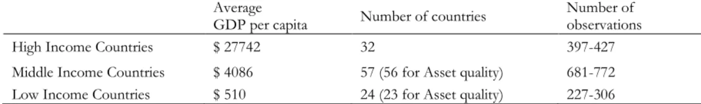
Table 6: Number of countries and observation per category Average

GDP per capita Number of countries Number of observations

High Income Countries $ 27742 32 397-427

Middle Income Countries $ 4086 57 (56 for Asset quality) 681-772 Low Income Countries $ 510 24 (23 for Asset quality) 227-306

When examining the effect that financial development has on energy consumption, researchers tend to focus on samples of countries within a certain category (Danish et al., 2018; Mehrara et al., 2015; Salim et al., 2014; Sadorsky, 2011, 2010; Tamazian et al., 2009). For this thesis, regional and income differences could play a part in how the banking sectors performance affects renewable energy consumption. Here on, the sample will be divided into three categories of high income countries, middle income countries and low income countries. Based on the World Bank’s World Development Indicator, the data material is divided into five income categories. For this thesis, these categories have been merged into three groups. Upper middle income countries and lower middle income countries are compressed into middle income countries. The data also consisted of two income categories for high income countries, one for OECD countries and one for non-OECD. Also these have been merged together. Table 6 gives a basic overview of the three income

(30)

categories and presents the number of countries and observations plus the average per capita GDP for each income group.

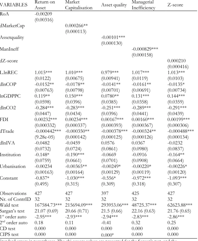
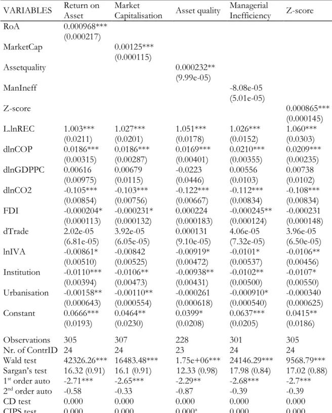
Table 7: Impact of banking sector performance on renewable energy consumption for high income countries

VARIABLES Return on _Asset Market _{Capitalisation} Asset quality Managerial _Inefficiency Z-score

RoA -0.00209 (0.00316) dMarketCap 0.000266** (0.000113) Assetquality -0.00101*** (0.000130) ManIneff -0.000829*** (0.000158) dZ-score 0.000210 (0.000416) L.lnREC 1.015*** 1.010*** 0.979*** 1.017*** 1.013*** (0.0122) (0.00675) (0.00941) (0.0119) (0.0103) dlnCOP -0.0152** -0.0178** -0.0141** -0.0161** -0.0135* (0.00763) (0.00798) (0.00701) (0.00691) (0.00734) lnGDPPC 0.119** 0.150*** 0.0780** 0.131*** 0.144*** (0.0598) (0.0396) (0.0385) (0.0358) (0.0359) dlnCO2 -0.284*** -0.283*** -0.251*** -0.289*** -0.291*** (0.0447) (0.0434) (0.0396) (0.0441) (0.0439) FDI 0.00232*** 0.00234*** 0.00167*** 0.00160*** 0.00199*** (0.000332) (0.000337) (0.000393) (0.000367) (0.000306) dTrade -0.000442*** -0.000350** -0.000378*** -0.000324** -0.000488*** (9.28e-05) (0.000142) (0.000125) (0.000126) (0.000134) dlnIVA -0.0482 -0.0459 0.0576 0.0367 -0.0232 (0.0732) (0.0724) (0.0861) (0.0980) (0.0837) Institution -0.148* -0.190*** -0.0669 -0.0916 -0.164** (0.0759) (0.0661) (0.0701) (0.0908) (0.0664) Urbanisation -0.00234 -0.00365** -0.00249* -0.00220* -0.00226* (0.00163) (0.00164) (0.00129) (0.00119) (0.00120) Constant -0.837* -1.030*** -0.556* -0.972*** -1.093*** (0.495) (0.315) (0.309) (0.318) (0.307) Observations 427 427 397 425 427 Nr. of ContrID 32 32 32 32 32 Wald test 167584.73*** 215694.09*** 293953.06*** 48725.37*** 62623.88*** Sargan’s test 21.07 (0.69) 20.66 (0.71) 21.5 (0.66) 22.16 (0.63) 21.76 (0.65) 1st_{order auto} _-2.95*** _-2.93*** _-2.94*** _-2.83*** _-2.86*** 2nd_{order auto} _0.18 _0.11 _-0.41 _0.32 _0.25 CD test 0.000 0.000 0.000 0.000 0.000 CIPS test 0.000 0.000 0.000a _0.000 _0.000

Standard errors in parentheses. The chi-square values are presented for the Sargan’s test, and the associated p-values are in parentheses. Z-values for the autocorrelation test are presented as well as the chi-square. P-values for the CD and CIPS tests are reported. a indicates instances where the CIPS test could not work in Stata and instead the ADF-test is used.